| Issue |
A&A
Volume 574, February 2015
|
|
|---|---|---|
| Article Number | A71 | |
| Number of page(s) | 15 | |
| Section | Interstellar and circumstellar matter | |
| DOI | https://doi.org/10.1051/0004-6361/201424657 | |
| Published online | 28 January 2015 | |
The HIFI spectral survey of AFGL 2591 (CHESS)
III. Chemical structure of the protostellar envelope⋆
1 SRON Netherlands Institute for Space Research, Landleven 12, 9747 AD Groningen, The Netherlands
e-mail: This email address is being protected from spambots. You need JavaScript enabled to view it.
2 Max-Planck Institute for Astronomy, Königstuhl 17, 69117 Heidelberg, Germany
3 Kapteyn Astronomical Institute, University of Groningen, PO Box 800, 9700 AV Groningen, The Netherlands
4 Universidad de Chile, Camino del Observatorio 1515, Las Condes, Santiago, Chile
5 Institute for Space Imaging Science, Department of Physics & Astronomy, University of Lethbridge, Lethbridge AB, Canada
Received: 23 July 2014
Accepted: 4 December 2014
Abstract
Aims. The aim of this work is to understand the richness of chemical species observed in the isolated high-mass envelope of AFGL 2591, a prototypical object for studying massive star formation.
Methods. Based on HIFI and JCMT data, the molecular abundances of species found in the protostellar envelope of AFGL 2591 were derived with a Monte Carlo radiative transfer code (Ratran), assuming a mixture of constant and 1D stepwise radial profiles for abundance distributions. The reconstructed 1D abundances were compared with the results of the time-dependent gas-grain chemical modeling, using the best-fit 1D power-law density structure. The chemical simulations were performed considering ages of 1−5 × 10⁴ years, cosmic ray ionization rates of 5−500 × 10-17 s-1, uniformly-sized 0.1−1 μm dust grains, a dust/gas ratio of 1%, and several sets of initial molecular abundances with C/O < 1 and >1. The most important model parameters varied one by one in the simulations are age, cosmic ray ionization rate, external UV intensity, and grain size.
Results. Constant abundance models give good fits to the data for CO, CN, CS, HCO+, H2CO, N2H+, CCH, NO, OCS, OH, H2CS, O, C, C+, and CH. Models with an abundance jump at 100 K give good fits to the data for NH3, SO, SO2, H2S, H2O, HCl, and CH3OH. For HCN and HNC, the best models have an abundance jump at 230 K. The time-dependent chemical model can accurately explain abundance profiles of 15 out of these 24 species. The jump-like radial profiles for key species like HCO+, NH3, and H2O are consistent with the outcome of the time-dependent chemical modeling. The best-fit model has a chemical age of ~10−50 kyr, a solar C/O ratio of 0.44, and a cosmic-ray ionization rate of ~5 × 10-17 s-1. The grain properties and the intensity of the external UV field do not strongly affect the chemical structure of the AFGL 2591 envelope, whereas its chemical age, the cosmic-ray ionization rate, and the initial abundances play an important role.
Conclusions. We demonstrate that simple constant or jump-like abundance profiles constrained with 1D Ratran line radiative transfer simulations are in agreement with time-dependent chemical modeling for most key C-, O-, N-, and S-bearing molecules. The main exceptions are species with very few observed transitions (C, O, C+, and CH) or with a poorly established chemical network (HCl, H2S) or whose chemistry is strongly affected by surface processes (CH3OH).
Key words: ISM: individual objects: AFGL 2591 / stars: formation / ISM: abundances / ISM: molecules / evolution / submillimeter: ISM
Herschel is an ESA space observatory with science instruments provided by European-led Principal Investigator consortia and with important participation from NASA.
© ESO, 2015
1. Introduction
The processes that produce massive stars are complex and not very well understood. This is mainly because massive stars are relatively rare: about 1% of stars are more massive than 10 M⊙. Their formation timescale is relatively fast and shorter, by a factor of ≳10, than for low-mass stars (Zinnecker & Yorke 2007). Moreover, massive stars remain deeply embedded for a considerable part of their lifetimes and usually form in clusters. While massive star-forming regions are typically several kiloparsecs away from our Sun, their challenging observations are the focus of many astrophysical investigations (see, e.g., Tan et al. 2014).
This paper focuses on AFGL 2591, a well-known, massive star-forming region with a circumstellar disk-like structure, bipolar outflows, and an extended envelope (van der Tak et al. 1999). It is a relatively isolated, deeply embedded, bright (L = 2 × 10⁵ L⊙, Sanna et al. 2012) object. It is located at a distance of 3.33 kpc, which has recently been accurately determined using trigonometric parallax measurements of H2O masers (Rygl et al. 2012).
According to the modern paradigm of massive star formation, AFGL 2591 can be classified as a high-mass protostellar object or an early “hot core” (Benz et al. 2007; Veach et al. 2013). The mass of the large-scale AFGL 2591 envelope is ~400 M⊙ (van der Tak et al. 2013). Inside this envelope, a cluster of B-type stars is being formed, which reveals itself as several continuum emission sources detected at cm wavelengths with Very Large Array (VLA 1, VLA 2, VLA 3, etc. Trinidad et al. 2003; van der Tak & Menten 2005; Jiménez-Serra et al. 2012a). The derived masses of these young stellar objects are ≲ 40 M⊙ (Jiménez-Serra et al. 2012a), and many of them are associated with prominent outflows (e.g., VLA 3). Among these sources, VLA 3 is one of the most massive objects (~ 38 M⊙), which dominates the AFGL 2591 spectral energy distribution and luminosity (Johnston et al. 2013).
Using the Plateau de Bure interferometer, Wang et al. (2012) observed AFGL 2591 VLA 3 in dust continuum and lines of HDO, H O, and SO2 at 0.5′′ resolution. Combining the data analysis with line radiative transfer calculations, they show that AFGL 2591 VLA 3 is surrounded by a massive disk with sub-Keplerian rotation and additional Hubble-like expansion motions. They also found that the observed molecular emission arises in various disk layers, with SO2 tracing the disk atmosphere and HDO and HO probing the disk mid-plane. Jiménez-Serra et al. (2012b) used 0.5′′ resolution observations toward AFGL 2591 VLA 3 with the Submillimeter Array (SMA) and discovered its radial chemical differentiation down to linear scales ≲ 3000 AU. The derived excitation temperatures of ~ 120 − 150 K and the gas kinematics are suggestive of a Keplerian disk surrounding a massive, 40 M⊙ star.
The physical structure of the circumstellar environment of AFGL 2591 was studied with single-dish submillimeter and infrared data as well as millimeter interferometry by van der Tak et al. (1999). Based on a 1D model with a power-law density profile with index 1.25, these authors estimated the abundances of CS, HCO+, HCN, and H2CS. The dust temperature due to heating by the young star was calculated to exceed 120 K at ~1500 AU from the star, so that the ice mantles are expected to be fully evaporated in the inner envelope.
From modeling of C17O emission lines, van der Tak et al. (2000b) inferred that around 40% −90% of the CO gas is depleted onto dust in the large-scale AFGL 2591 envelope. Their results suggest that freeze-out and thermal desorption control the gas-phase abundance of CO. van der Tak et al. (2003) observed sulfur-bearing molecules in several massive protostellar envelopes, and derived column densities and abundances of H2S, SO, SO2, H2CS, HCS+, NS, OCS, and CS in AFGL 2591. These results are consistent with a model of ice evaporation in the envelope with gradients in temperature and density, and a chemical age of ~ 105 years.
Bruderer et al. (2010b) used the HIFI instrument onboard the Herschel satellite and detected emission lines of light hydrides such as CH, CH+, NH, OH+, and H2O+. They found that observed abundances and line excitation of CH and CH+ can be explained with an envelope-outflow model, where far-ultraviolet (FUV) stellar radiation irradiates and heats the outflow walls, driving the gas-phase, photon-dominated chemistry that produces these molecules.
Using these large observational data sets of the AFGL 2591 molecular content, a number of theoretical studies of its chemical and physical evolution have been performed. The study of the envelope AFGL 2591 by Doty et al. (2002) was based on a 1D thermal and gas-phase chemical model of the observed abundances and column densities for 29 species. They were able to explain most of the chemical structures and found hints of high-temperature nitrogen and hydrocarbon chemistry. They also derived that most of the sulfur in the cold gas should be locked in CS, in SO2 in the warm gas, and S in the hot gas. From the observed abundances of HCO+ and N2H+ and the cold gas-phase production of HCN the cosmic-ray ionization rate was constrained, ~ 5 × 10-17 s-1. The derived best-fit chemical age is between 7000 and 50 000 years.
Stäuber et al. (2004, 2005) analyzed the influence of FUV and X-ray radiation from massive young stellar objects on the chemistry of its envelope. The UV flux seems to affect only the regions within 500−600 AU from the star, but X-rays can penetrate larger distances. They both enhance the abundance of simple hydrides, ions, and radicals.
Bruderer et al. (2009a,b, 2010a) introduced a 2D model with a self-consistent calculation of the dust temperature, a fast chemical method, and a multi-zone escape probability method for the line radiative transfer. They benchmarked the feasibility of this model by comparing it with published models of the AFGL 2591 protostellar envelope. Bruderer et al. (2010b) utilized this 2D model to investigate the effects of the cavity shapes, outflow densities, and disk properties on the large-scale chemical composition of AFGL 2591. They derived that the Herschel observations of diatomic hydrides and hydride ions can be explained by the outflow model with the walls directly irradiated by the stellar FUV photons, producing high gas temperatures and rapid photodissociation of their saturated parent species.
We observed AFGL 2591 with the Heterodyne Instrument for the Far-Infrared (HIFI, De Graauw et al. 2010) on board the ESA Herschel Space Observatory (Pilbratt et al. 2010) as a part of the HIFI/CHESS guaranteed time key programme (Chemical Herschel Survey of Star Forming Regions, Ceccarelli et al. 2010). A full spectral survey of AFGL 2591 of HIFI bands 1a−5a (480−1240 GHz) was obtained. Nine additional selected frequencies were observed; the corresponding bands are 5b (lines: HCl and CO), 6a (CO), 6b (CO), 7a (NH3, CO), and 7b (CO, OH, [CII]). These observations were supplemented with several lines from the ground-based James Clerk Maxwell Telescope (JCMT)1 as part of the JCMT Spectral Legacy Survey (SLS, Plume et al. 2007; van der Wiel et al. 2011).
The results from our spectral survey are presented in a series of three papers. The first paper focused on highly-excited linear molecules (van der Wiel et al. 2013, Paper I). We analyzed the lines profiles of CO isotopologues, HCO+, CS, HCN, and HNC in the FIR/mm range by using a 1D non-LTE line radiative transfer model. It was found that a spherical envelope model is able to fit the upper-state transitions at Eul/k> 150 K for all species, and that an additional hot, optically thin gas component (such as from an outflow cavity wall) is required. In the second paper the entire survey was summarized (Kaźmierczak-Barthel et al. 2014, Paper II). A simple excitation analysis was also performed to estimate column densities and excitation temperatures for a multitude of observed molecules. In total, we identified 32 species (including isotopologues), with 268 emission and 16 absorption lines (excluding blended lines). The derived molecular column densities range from 6 × 1011 cm-2 to 1019 cm-2 for N2H+ and CO, and excitation temperatures range from 19 to 175 K for HCO+ and SO2, respectively. We have distinguished two gas components, namely cold gas traced by e.g., HCN, H2S, and NH3 (T ≲ 70 K) and warm gas traced by e.g., CH3OH and SO2 (T> 70 − 100 K).
In the present work (Paper III), we are going one step further in the analysis of our spectral survey. Here, all molecules observed in the protostellar envelope are modeled using the radiative transfer code RATRAN (Hogerheijde & van der Tak 2000) together with a time-dependent gas-grain chemical model based on the alchemic code (Semenov et al. 2010).
This paper is organized as follows. Section 2 presents a radiative transfer analysis of molecules observed in the protostellar envelope of AFGL 2591, based on all data listed in Paper II, and Sect. 3 describes the chemical modeling. Discussion of our results and comparison between these two approaches is given in Sect. 4, and our conclusions follow in Sect. 5.
2. Radiative transfer modeling
2.1. One-dimensional physical model
The model for the physical structure of the envelope of AFGL 2591 is based on the study of van der Tak et al. (2013). It uses the new distance of 3.3 kpc and the corresponding luminosity of L = 2 × 10⁵ L⊙. The previous distance estimates were uncertain, with values between 1 and 2 kpc (e.g., van der Tak et al. 1999, 2000b), thus the luminosity at 1 kpc is L = 2 × 10⁴ L⊙. The radial density profile was derived from the JCMT/SCUBA2 (450, 850 μm) and the Herschel/PACS3 (70, 100, 150 μm) data with the radial density power-law index of α ~ 1, assuming a power-law density profile n(r) ∝ r− α. The physical model consists of 50 shells, with temperatures of 1383 K and 29 K in the inner and outer shells, respectively, and a total gas mass of 373 M⊙. The temperature and density structure of the model are presented in Fig. 1.
The results presented in this paper are based on a slightly different physical model of AFGL 2591 from that described in Paper I (van der Wiel et al. 2013). The model from Paper I was based only on the SCUBA data; here the PACS data were added (for the modeling procedure see van der Tak et al. 2013), and so all molecular abundances from the Papers I and III were recalculated with the new physical model that is based on the combined SCUBA and PACS data sets.
2.2. Line modeling
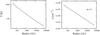 |
Fig. 1 Temperature and density structure of the 1D physical model of AFGL 2591. |
Spherically symmetric radiative transfer calculations with the Monte Carlo RATRAN code (Hogerheijde & van der Tak 2000) were run to estimate abundances of observed species in the protostellar envelope of AFGL 2591. Spectroscopic and collisional parameters were taken from the lamda4 database (Leiden Atomic and Molecular Database, Schöier et al. 2005). Detailed information about the adopted collisional rate coefficients for each molecule is given in Sect. 2.4.
As a first step, abundances were estimated assuming a constant relative abundance throughout the protostellar envelope. To find the best-fit values of the abundances, observed and synthetic line fluxes were compared using χ2-minimization. The constant-abundance models agree with the data of several molecules in terms of the total line flux and the shape of the line.
However, modeling the observed lines with a constant abundance may not always be the correct approach. Laboratory studies indicate that many molecules reside in more or less volatile ice mantles on dust grain surfaces at temperatures below 20 − 110 K depending on species, surface composition, and structure (see, e.g., Van Dishoeck & Blake 1998; Bisschop et al. 2006, Herbst & van Dishoeck 2009; Fayolle et al. 2011b). Usually, water ice is a major solid component that entraps other heavy ices and a fraction of volatile ices such as CO. Hence, models with jump-like abundance profiles at ~100 K may better represent the observations of gas-phase species in warm environments.
Schöier et al. (2002) performed detailed 1D radiative transfer analysis of the observed continuum and lines toward the young stellar object IRAS 16293-2422. They concluded that the lines of some molecules, e.g., H2CO, CH3OH, SO, SO2, and OCS can only be explained when their abundances are greatly increased in warm regions of the envelope, where ices are expected to thermally evaporate. Jørgensen et al. (2004) derived that in low-mass pre- and protostellar objects, the spectra of nitrogen-bearing species together with HCO+ and CO cannot be fitted with a constant abundance and require a model with a radial chemical gradient, where the region with molecular freeze-out is represented by a jump-like drop of the molecular abundances. van der Tak et al. (2006) studied water line spectra in the envelopes and disks around young massive stars and found that the water abundance is lower outside a critical radius, which corresponds to a temperature of ~ 100 K.
According to the chemical study of Rodgers & Charnley (2001), the temperature of 230 K is also important, and may cause another sudden, jump-like rise in the abundances of N-bearing species. Their chemical model predicts that high-temperature neutral-neutral reactions of O and OH with H2 drive the remaining oxygen that is not bound in CO into H2O. This partly breaks the chemical cycling between N2 and N, where N2 (which is constantly destroyed by ionized He atoms) is reformed by rapid reactions of released N with OH first into NO and NH, and then back to N2. As a result, at T ≳ 230 K abundances of major N-bearing molecules become greatly enhanced. Boonman et al. (2001) have analyzed the HCN J = 9 − 8 spectrum from the AFGL 2591 envelope and found that the HCN abundance above the temperature of 230 K should be at least 2 orders of magnitude higher than in the colder region.
Thus, in the present study of the protostellar envelope of AFGL 2591, the observations of each molecule are analyzed in the framework of the constant abundance model as well as models with jumps at 100 K and 230 K. The molecular abundances were estimated from the analysis of the optically thin isotopologue lines if their observations were available. We used the standard isotopic ratios: 12C/13C = 60, 16O/18O = 500, 16O/17O = 2500, 14N/15N = 270, and 32S/34S = 22 (Wilson & Rood 1994).
2.3. Error budget
2.3.1. Molecular data
One of the largest sources of uncertainty for radiative transfer analysis are molecular data, especially collisional rate coefficients. Schöier et al. (2005) and van der Tak (2011) describe in detail the accuracy of molecular data needed for radiative transfer analysis, such as collisional rate coefficients, spontaneous emission probabilities, transition frequencies, statistical weights, and energy levels. The uncertainties involved in determining collisional rate coefficients are summarized by Flower (1990), Roueff (1990), and Roueff & Lique (2013). The determination of collisional rate coefficients includes uncertainties that vary for different species. First, there is an inconsistency in the astrophysical literature regarding choices of values of electric dipole moments for some molecules, which may cause an error of a factor of two in their derived abundances (Schöier et al. 2005). Second, published collisional rate coefficients often cover only a limited range of temperatures and energy levels, and extrapolation of their values outside of these ranges may cause additional errors (van der Tak 2011). Third, many molecules do not have calculated collisional rate coefficients at all or have the collisional data available only for collisions with e−, He, or H2J = 0 (Schöier et al. 2005). For some molecules it is possible to scale rates obtained for a molecule with similar structure, using the reduced mass (see Eq. (12), Schöier et al. 2005). Such scaling can be dangerous when collisional rates with helium are used as a proxy for the H2 collisional rates. In addition, for freshly formed or hot H2 gas collisions with H2, J = 1 can become important to properly describe the level populations, which is often ignored in astrophysical modeling. All together, these uncertainties may cause the estimated abundances to have error bars of 20% and probably higher.
2.3.2. Physical model
The uncertainties associated with the physical model of AFGL 2591 mostly depend on the estimation of the envelope mass, density profile, and distance to the object (van der Tak et al. 2013). The distance to AFGL 2591, d = 3.33 ± 0.11 kpc, has been quite accurately determined thanks to the VLBI parallax measurements of 22 GHz water maser emission (see Rygl et al. 2012). The influence of the envelope masses and density profiles on the physical model were analyzed in the same way as described in Sect. 5.5 of Herpin et al. (2012). In our model, the main uncertainties arise from the adopted dust opacities. Hence, we performed test SED modeling taking these uncertainties into account and found that the resulting CO abundances in the AFGL 2591 envelope can differ by a factor of ~3, which is the dominant factor. However, this parameter affects all our abundance estimates equally, so that the relative abundances between species are unchanged.
2.3.3. Observational data
Regarding observational uncertainties, we have to take into account errors from the measurements of the integrated line intensities, because these values were iteratively compared with the modeled line fluxes to identify a best-fit model. For strong lines (e.g., CO), calibration errors dominate the uncertainty. For Herschel data this is ~10%; for the ground-based data the calibration uncertainties are more than 20%. For weak lines, spectral noise dominates the error, which amounts to 50−100 mK depending on frequency. All in all, the total error is the maximum of these contributions.
The other factor that affects the accuracy of estimated abundances is the number of observed transitions for a given molecule. The abundances of a species can be calculated more precisely when observations of different lines from many energy levels are available, such as many different transitions of CO and its isotopologues. On the other hand, for NO, OCS, OH, H2CS, C, C+, CH, and O, observations of only one or two lines are available. Consequently, the uncertainties of their best-fit abundances are higher.
Abundances (relative to H2) estimated with the spherical radiative transfer model (RATRAN) for the envelope of AFGL 2591, based on HIFI and JCMT data.
2.4. Derived abundances of analyzed species
In Table 1 the best-fitting values of abundances for observed species in the protostellar envelope of AFGL 2591 are presented. The table is divided into five parts, corresponding to the five following subsections in which we discuss the modeled species.
In the first part of Table 1 (Sect. 2.4.1) molecules (CO, CN, and CS) for which a constant model gave the best-fitted abundance are listed. Moreover, for these species we observed many transitions from different energy levels, so it was possible to exclude models with jumps at 100 K and 230 K.
The second part of Table 1 (Sect. 2.4.2) consists of species (HCO+, H2CO, N2H+, and CCH) for which a constant model gave as good a fit to the observed fluxes as a model with a jump at 100 K, with a lower abundance in the inner part of the envelope. For these four molecules, the best-fit constant model gives the same abundance as is derived in the outer part of the envelope from the model with a jump. The lower inner abundance was predicted by chemical models and then applied to RATRAN. Both models, constant and with a jump, reproduce very well our observed integrated line intensities. We also observed several transitions from different energy levels of these molecules, so it was possible to exclude jump models with a higher inner abundance.
Part 3 of Table 1 presents species (NO, OCS, OH, H2CS, C, C+, CH, and O) for which a constant model also gave the best-fit abundance; however, it is not possible to exclude a jump model because of the lack of different observed transitions. Usually, for these species we observed only one line or a few lines (Sect. 2.4.3), which causes higher uncertainties in the derived abundances of these species, up to a factor of 12 for CH and C.
Only two molecules are listed in the fourth part of Table 1 (Sect. 2.4.4), HCN and HNC. The model with an abundance jump at 230 K was found to provide the best-fit value of χ2. This is consistent with the results of Boonman et al. (2001) for HCN.
In the last part of Table 1 (Sect. 2.4.5) we list the molecules (NH3, SO, SO2, H2S, H2O, HCl, and CH3OH) for which the model with jump at 100 K provided the best fit. The constant models were run first for these molecules, but they either did not reproduce the observed line fluxes (SO, SO2, and CH3OH) or made some lines appear in absorption (NH3, H2S, H2O, and HCl).
2.4.1. Constant abundance model with many transitions
In this section we discuss species (CO, CN, and CS) modeled by a constant abundance model (first part of Table 1). For these species we observed many transitions from different energy levels, and models with jumps at 100 K and 230 K were excluded.
Carbon monoxide is one of the most widely studied and well-known molecules. Because of its importance as a molecular tracer, detailed and accurate CO molecular data are available. For this work, we adopted the collisional rate coefficients for CO with H2 from Yang et al. (2010), which cover energy levels up to J = 40 for temperatures ranging from 2 K to 3000 K. We estimate a CO abundance relative to H2 of 2 × 10⁻⁴, which is the same value as previously calculated by van der Tak et al. (1999), although the two results are based on different physical models. Our result was based on observations of 31 lines of CO and its isotopologues (13CO, C18O, and C17O); however, taking into account the possible sources of uncertainties, the overall CO abundance uncertainty was estimated to be a factor of 3.
Collisional rates for CN with He were calculated by Lique et al. (2010); the scaled rates for collisions with H2 were adopted from the lamda database. We obtained an abundance of 1 × 10⁻⁹ with the uncertainty within a factor of 5. Stäuber et al. (2007) estimated a higher CN abundance of 2.3 × 10⁻⁸ by using a different physical model and assuming a distance of d = 1 kpc. These authors also tested models with a jump in abundance at 100 K and estimated an outer abundance of 10-9 and an inner abundance of 6 × 10⁻⁷. However, the two models were statistically indistinguishable. Stäuber et al. (2007) based their calculations on seven hyper-fine components from Eup~ 33 K. Our estimations of the CN abundance are based on several CN lines from three different energy levels of Eup ~ 33, 82, and 114 K and are thus more robust. The overall CN abundance uncertainty is estimated to be a factor of 3.
We scaled the rate coefficients for collisions of CS and H2 from collisions of CS with He, which were taken from Lique et al. (2006b). Based on observations of several lines of CS from energy levels of Eup = 66 − 282 K and its two isotopologues, 13CS and C34S, we derived a CS abundance of 4 × 10⁻⁸. The uncertainty of this estimation is within a factor of 4. van der Tak et al. (2000b) estimated a slightly lower abundance, [CS] = 1 × 10⁻⁸, but using the old distance and an outdated model.
2.4.2. Model with a lower inner abundance
In this section we discuss species (HCO+, H2CO, N2H+, and CCH) fitted by a model with an abundance jump at 100 K, with a lower inner abundance (second part of Table 1). This model gives an equally good fit to the observational fluxes as a constant abundance model. The lower abundance in the inner part of the envelope was predicted by chemical models (Sect. 3.1).
Collisional rates for HCO+ with H2 were taken from Flower (1999). From RATRAN calculations we derived, with the uncertainty within a factor of 4, the following HCO+ abundances: [HCO+] = 3 × 10-11 in the inner part of the envelope (where T> 100 K) and [HCO+] = 3 × 10⁻⁸ in the outer region of the envelope (T< 100 K). The outer abundance is very similar to the value calculated by van der Tak et al (1999): 1 × 10⁻⁸.
The collisional rates for H2CO with H2 were taken from Wiesenfeld & Faure (2013). Based on 17 H2CO transitions from a broad range of energy levels (Eup = 32−236 K), we derived an abundance of 1 × 10-11 and 1 × 10⁻⁸ in the inner and outer envelope with the uncertainty of a factor of 4. The ortho-to-para ratio is 3:1 for H2CO, thus models for o-H2CO and p-H2CO were run separately and then both abundances were added to get a total H2CO abundance. Based on the old distance and physical model, van der Tak et al. (1999, 2000b) estimated the H2CO abundance in the range of 2 − 4 × 10⁻⁹ which is between our values.
The collisional rate coefficients for N2H+ with H2 were adopted from the lamda database, where they were scaled from the rates for HCO+ from Flower (1999). Based on three observed lines, we obtained N2H+ abundances of 8 × 10-13 and 8 × 10⁻¹⁰ in the inner and outer part of the envelope, respectively, with an uncertainty of a factor of 5.
The rate coefficients for collisions of CCH with H2 were scaled from collisions of CCH with He, which were adopted from Spielfiedel et al. (2012). We used eight lines from four different energy levels and derived an abundance of 8 × 10-12 and 8 × 10⁻⁸ in the inner and outer parts of the envelope. The error of this estimation is a factor of 4.
2.4.3. Constant abundance model with a few transitions
In this section we discuss species (NO, OCS, OH, H2CS, C, C+, CH, and O) that were modeled by a constant abundance model (third part of Table 1). For these species we observed only one or two transitions from different energy levels. Thus, the precision of the estimated abundances is lower and models with a jump at 100 K or 230 K cannot be excluded.
The collisional rate coefficients for NO with H2 were adopted from the lamda database, where they were scaled from the rates for NO with He by Lique et al. (2009). We obtained abundances of [NO] = 5 × 10⁻⁸ and a very similar value was estimated by Stäuber et al. (2007), [NO] = 3.1 × 10⁻⁸. However, our calculations are based on only four lines from two different energy levels, which causes uncertainties that are higher by a factor of ~8. We also used a different physical model than Stäuber et al. (2007).
The collisional rates for OCS were adopted from Green & Chapman (1978). Flower (2001) calculated the rate coefficients for collisions of OCS (J ≤ 29) with He at low temperatures (T ≤ 150 K) and found that their results are comparable with those for collisions between OCS and p-H2 derived by Green & Chapman (1978). We derived an abundance of 4 × 10⁻⁸, which is a very similar value to that previously calculated by van der Tak et al. (2003), 1 × 10⁻⁸. However, we also consider this result to be very uncertain (a factor of 8) because this estimation is based on only three lines from very similar energy levels.
The collisional rate coefficients for OH with H2 were taken from Offer et al. (1994). We derived [OH] = 2 × 10⁻⁸, but this estimation is very uncertain (a factor of 8), because it is based on fitting the observations of only one transition.
We scaled the collisional rate coefficients for H2CS from the rates for H2CO, which were taken from Wiesenfeld & Faure (2013). We derived [H2CS] = 4 × 10⁻⁹. This result is also uncertain by a factor of 8 because it is based on only three lines from very similar energy levels. All three observed lines belong to o-H2CS. The total H2CS abundance was calculated assuming an ortho-to-para ratio of 3:1. van der Tak et al. (2003) derived a lower H2CS abundance, 3 × 10⁻¹⁰, using older molecular data, and an old physical model using the old distance.
Rate coefficients for collisions of C atoms with H2 were taken from Schröder et al. (1991). Based on two observed transitions, we derived [C] = 4 × 10⁻⁶ with an error of a factor of ~8.
Rate coefficients for collisions for C+ with H2 were adopted from Flower & Launay (1977). We derive a C+ abundance of 7 × 10⁻⁶. This result is highly uncertain (a factor of ~12), again because it is based only on one observed transition. Moreover, the C+ line profile is contaminated by emission from the off-position, even after applying corrections, which causes a higher error of the measurements (see Appendix of Paper II).
Currently, accurate collisional rates for CH do not exist, so we scaled OH collisional rate coefficients (Offer et al. 1994). This scaling may cause significant errors, in particular because CH and OH do not have the same electronic structure. Hence we consider our abundance estimate of 1 × 10⁻⁸ as highly uncertain (a factor of ~12).
Rate coefficients for collisions for O with H2 were taken from Jaquet et al. (1992). The derived O abundance is 2 × 10⁻⁵ with an error of a factor of ~12. This calculation is based on the observation of one line (145.525 μm), from the “Water In Star forming regions with Herschel” (WISH) Project, made with PACS (Woojin Kwon, priv. comm.).
2.4.4. Models with a jump at 230 K with a higher inner abundance
In this section we discuss two species, HCN and HNC (fourth part of Table 1). The collisional rate coefficients for HCN and HNC with H2 were adopted from the lamda database, where they were scaled from values with He by Dumouchel et al. (2010).
To estimate the abundances of HNC, HCN, and their isotopologues, a model with an abundance jump at 230 K was adopted. Boonman et al. (2001) used a model with a jump at 230 K, because this temperature was predicted by chemical models as the temperature above which most of the atomic oxygen is driven into water. As a result abundances of C- and N-bearing species are higher, and derived abundances are 5 × 10⁻⁶ and 5 × 10⁻⁷ for HCN, and 1 × 10⁻⁷ and 1 × 10⁻⁸ for HNC, in the inner (where T < 230 K) and outer regions of the envelope. The abundance uncertainty is estimated to be within a factor of 4 for HCN and 5 for HNC. These results are similar to Boonman et al. (2001) who found [HCN] = 1 × 10⁻⁶ in the inner, hot envelope and [HCN] = 1 × 10⁻⁸ in the outer part of the envelope. We conclude that jump models reproduce observational lines of HCN much better than models with a constant abundance, especially when multiple transitions are observed.
2.4.5. Models with a jump at 100 K with a higher inner abundance
In this section we discuss species (NH3, SO, SO2, H2S, H2O, HCl, and CH3OH) modeled with an abundance jump at 100 K, with a higher inner abundance (the last part of Table 1).
The collisional rate coefficients for NH3 with H2 were adopted from Danby et al. (1988). More accurate potentials exist (Maret et al. 2009), but they cover a smaller temperature range and do not include hyperfine structure. For ammonia, the best-fit model was with an abundance jump at ~100 K. Models with the same abundances for o-NH3 and p-NH3 were run separately. The expected ortho-to-para ratio is 1:1 for NH3, so both abundances were added to get a total ammonia abundance. From the RATRAN calculations we derived, with an uncertainty of a factor of 4, an ammonia abundance of [NH3] = 4 × 10⁻⁶ in the inner part of the envelope (where T> 100 K) and [NH3] = 4 × 10⁻¹⁰ in the outer region of the envelope (where T< 100 K). Previously, Takano et al. (1986) derived [NH3] ~ 10-8 by assuming a constant abundance. A model with a jump seems to be more accurate for our data set.
The rate coefficients for collisions of SO with H2 were scaled from collisions of SO with He, which were taken from Lique et al. (2006a). Based on 22 SO transitions from a broad range of energy levels (Eup = 26−405 K) and three 34SO lines we derived an abundance of 5 × 10⁻⁷ in the inner part of the envelope and 5 × 10⁻⁹ in the outer region of the envelope (where T< 100 K). The uncertainty of this estimation is within a factor of 4. van der Tak et al. (2003), using six lines from energy levels Eup = 35−88 K, estimated a constant SO abundance of 1 × 10⁻⁸. A model with an abundance jump is necessary to fit our SO lines from a broad energy range.
The collisional rate coefficients for SO2 with H2 were taken from Green (1995). The most recent calculations of collisional rates were made by Cernicharo et al. (2011), but they included only temperatures up to 30 K. This calculation is limited to cold interstellar clouds; however, it shows that collisions with molecular hydrogen are about 3 times more effective in exciting SO2 than helium, even after scaling for the reduced mass, because the long-range interaction is significant. Thus, we scaled the data from Green (1995) by multiplying them by a factor of 3. Based on 50 observed SO2 lines from a broad range of energy levels (Eup = 31−354 K) and five 34SO2 transitions we derived an abundance of 5 × 10⁻⁶ in the inner part of the envelope and 5 × 10⁻⁹ in the outer region of the envelope. The uncertainty of this estimation is within a factor of 5. van der Tak et al. (2003) estimated a constant abundance of [SO2] = 2 × 10⁻⁹ that is similar to our abundance from the outer part of the envelope; however, the jump is needed to fit our observational data.
We scaled the collisional rate coefficients for H2S from the rates for H2O, which were taken from Dubernet et al. (2006) and Daniel et al. (2011). The ortho-to-para ratio is 3:1 for H2S; thus, models for o-H2S and p-H2S were run separately and then both abundances were added to get a total H2S abundance. We derived an abundance of 8 × 10⁻⁸ in the inner part of the envelope and 8 × 10⁻¹⁰ in the outer region of the envelope. The uncertainty of this estimation is within a factor of 5. van der Tak et al. (2003), based on three lines from Eup = 28−84 K, estimated [H2S] = 8 × 10⁻⁹. A model with a jump seems to be more accurate for our data set.
The collisional rate coefficients for H2O were taken from Dubernet et al. (2006) and Daniel et al. (2011). To get a total water abundance, we added results from two models for o-H2O and p-H2O, assuming an o/p ratio of 3:1. The estimated H2O abundance is 1 × 10⁻⁴ in the inner part of the envelope and 1 × 10⁻⁹ in the outer region of the envelope. The uncertainty of this estimation is within a factor of 4. van der Tak et al. (2006), from a constant abundance model, derived [H2O] = 6 × 10⁻⁵ and from a jump model the value of 1.4−2 × 10⁻⁴ and 10-6 − 10-8 in the inner and outer part of the envelope, respectively. Both results are very similar, although they are based on different physical models. See Choi et al. (2014) for further discussion of the H2O abundance in the envelope of AFGL 2591.
The collisional rate coefficients for HCl with H2 were adopted from the lamda database, where they were scaled from the rates for HCl with He by Neufeld & Green (1994). We derived an abundance of 4 × 10⁻⁶ in the inner part of the envelope and 4 × 10⁻¹⁰ in the outer region of the envelope. This estimation is based on only five detected HCl lines, three hyper-fine components from the energy level of Eup= 30 K and two from the higher state Eup = 90.1 K, thus the uncertainty of this estimation is higher, within a factor of 8.
The collisional rates for CH3OH with H2 were taken from Rabli & Flower (2010). Data are available for both A- and E-type CH3OH, but given the many CH3OH lines in our spectra, we used only transitions of A-type CH3OH, assuming a ratio of A/E = 1:1, which is appropriate at the high (>30 K) temperature in the AFGL 2591 envelope. To obtain the total methanol abundance we multiplied our estimate for A-type CH3OH by 2. We estimated an abundance of 8 × 10⁻⁷ and 8 × 10⁻⁸ in the inner and outer part of the envelope, respectively. The uncertainty of this estimation is within a factor of 4. van der Tak et al. (2000a) derived a slightly lower CH3OH abundance, 8 × 10⁻⁸ in the inner part of the envelope and 2 × 10⁻⁹ in the outer part of the envelope. This calculation is based on old collisional rate coefficients and an old physical model.
3. Theoretical modeling
3.1. Chemical model
Our chemical model is based on the advanced time-dependent chemical kinetics alchemic code (see Semenov et al. 2010). The gas-grain deuterium chemistry network of Albertsson et al. (2013, 2014) is utilized. The non-deuterated chemical network is based on the osu.2007 rate file5. The network is supplied with a set of approximately 1000 reactions with high-temperature barriers from Harada et al. (2010, 2012). The recent updates as of June 2013 to the reaction rates are implemented (e.g., from the kida database6; see Wakelam et al. 2012; Albertsson et al. 2013).
Primal isotope exchange reactions for H as well as CH and C2H
 from Roberts & Millar (2000), Gerlich et al. (2002), Roberts et al. (2004), and Roueff et al. (2005) were included. In cases where the position of the deuterium atom in a reactant or in a product was ambiguous, a statistical branching approach was used. In Albertsson et al. (2014) this deuterium network was further extended by adding ortho and para forms of H2, H
 , and H isotopologues and the related nuclear spin-state exchange processes from several experimental and theoretical studies (Gerlich 1990; Gerlich et al. 2002; Flower et al. 2004, 2006; Walmsley et al. 2004; Pagani et al. 2009; Hugo et al. 2009; Honvault et al. 2011; Sipilä et al. 2013).
In our standard model, we used the cosmic ray (CR) ionization rate ζCR = 5 × 10-17 s-1, as derived by van der Tak & Van Dishoeck (2000) specifically for AFGL 2591. In addition, we considered two other models where the CR ionization rate was increased by factors of 10 and 100.
Several tens of newer photoreaction rates are adopted from Van Dishoeck et al. (2006)7. In the standard model, the AFGL 2591 envelope is assumed to be bathing in an ambient interstellar FUV field with an intensity of one Draine (1978) interstellar UV. In addition, we considered two other models where the UV intensity (in Draine’s unit of χ0) was assumed to be 50 and 500. The self- and mutual-shielding of CO and H2 from external dissociating radiation was calculated as in Semenov & Wiebe (2011).
The grains are uniform amorphous olivine particles with a density of 3 g cm-3 and a radius of 0.1 μm. Each grain provides around 1.88 × 10⁶ surface sites (Biham et al. 2001). Two models with smaller (0.03 μm) and bigger (1 μm) uniform grains were also considered.
The gas-grain interactions include sticking of neutral species and electrons to dust grains with 100% probability and desorption of ices by thermal, CR-, and UV-driven processes. We do not allow H2 isotopologues to stick to grains because for H2 this requires temperatures of ≲ 4 K. A UV photodesorption yield of 3 × 10⁻³ was adopted (e.g., Öberg et al. 2009a,b; Fayolle et al. 2011a, 2013). Photodissociation processes of solid species are taken from Garrod & Herbst (2006) and Semenov & Wiebe (2011).
Surface recombination proceeds through the classical Langmuir-Hinshelwood mechanism (e.g., Hasegawa et al. 1992). The ratio between diffusion and desorption energies of surface reactants is taken to be 0.7 for all surface species (Ruffle & Herbst 2000). We do not allow tunneling of surface species via the potential wells of the adjacent surface sites. To account for hydrogen tunneling through barriers of surface reactions, we employed Eq. (6) from Hasegawa et al. (1992), which describes a tunneling probability through a rectangular barrier with thickness of 1 Å.
For each surface recombination, we assume a 1% probability for the products to leave the grain as a result of the partial conversion of the reaction exothermicity into breaking the surface-adsorbate bond (Garrod et al. 2007; Vasyunin & Herbst 2013b). Following experimental studies on the formation of molecular hydrogen on amorphous dust grains by Katz et al. (1999), the standard rate equation approach to the surface chemistry is adopted. In addition, dissociative recombination and radiative neutralization of molecular ions on charged grains and grain recharging are taken into account.
Overall, the chemical network consists of 1268 species made of 13 elements and 38 812 reactions. With this network and using 10-5 relative errors and 10-15 absolute errors, the AFGL 2591 model takes about 3 min of CPU time (Core-i7 2.0 GHz, gfortran 4.8-x64) to calculate over an evolutionary time span of 1 − 10× 104 years (with 99 logarithmic time steps), which was proposed by Stäuber et al. (2005) as the chemical age of AFGL 2591.
3.2. Initial abundances
Initial abundances (relative to total H) for modeling pre-AFGL 2591 evolutionary phase.
Top 25 of the initially abundant molecules (relative to total H) for the AFGL 2591 chemical modeling.
To set the initial abundances of the model, we calculated the chemical evolution of a 0D molecular cloud with nH = 2 × 104 cm-3, T = 10 K, and AV = 10 mag over 1 Myr. The neutral “low metals” (model lm) elemental abundances of Graedel et al. (1982), Lee et al. (1998), and Agúndez & Wakelam (2013) were used, with the solar ratio of C/O = 0.44, initial ortho/para H2 of 3:1, hydrogen being fully in molecular form, and deuterium locked in HD (see Table 2). The resulting abundances of modeling this pre-AFGL 2591 phase were used as initial abundances for the AFGL 2591 chemical modeling (see Table 3). The instantaneous jump from a 0D to a 1D structure is a crude approximation which future work should address in more detail.
In addition to the lm abundance set, we considered several initial molecular abundance sets with non-solar C/O ratios, which were proposed to explain observed peculiarities of the sulfur and oxygen chemistries in high-mass star-forming regions and protoplanetary disks (Hincelin et al. 2011; Dutrey et al. 2011), called d11c and h11 (see Table 2). Both these elemental abundance sets have C/O > 1, an abundance of nitrogen 3 times higher than in our standard lm set, and most of the atoms in the ionized state. In addition, the set of Dutrey et al. (2011) has a 10 times lower sulfur abundance than the lm set.
Similar to our standard lm model, we calculated the chemical evolution of a 0D molecular cloud to set the initial abundances for the 1D physical-chemical model of the AFGL 2591 envelope (see Table 3) with the two non-solar C/O initial abundances. The physical parameters of both models were the same, nH = 2 × 105 cm-3, T = 15 K, and AV = 10 mag, and we adopted an age of 50 kyr. These physical conditions differ from the lm case presented above. Since AFGL 2591 is forming a cluster of low- and intermediate-mass stars, it is not obvious which physical conditions more adequately describe the pre-AFGL 2591 phase, namely, those characteristic of low-mass prestellar cores or those characteristic of higher-mass infrared dark clouds. The two d11c and h11 models correspond to the high-mass case, whereas the lm model corresponds to the low-mass case.
The initial abundances calculated with this 0D physical model and the Dutrey et al. (2011, their model C) elemental set is called d11c. Similarly, the model of initial elemental abundances of Hincelin et al. (2011) adopted to calculate pre-AFGL 2591 the initial abundances is called h11 (see Table 3).
3.3. Error estimations
The difficulty of calculating abundance uncertainties is well known in chemical studies of various astrophysical environments, ranging from dark clouds and hot cores to protoplanetary disks and exoplanetary atmospheres (see, e.g., Agúndez & Wakelam 2013; Dobrijevic et al. 2003; Vasyunin et al. 2004, 2008; Wakelam et al. 2005, 2006). The error budget of the theoretical abundances is determined by both the uncertainties in physical conditions in the object and, to a larger degree, by uncertainties in the adopted reaction rate coefficients and their barriers. Poorly known initial conditions for chemistry may also play a role here.
In order to estimate the chemical uncertainties rigorously one needs to perform a large-scale Monte Carlo modeling by varying the reaction rates within their error bars and recalculating the chemical evolution of the specific astrophysical environment. We do not attempt to perform such a detailed study and use the estimates from previous works.
Previous studies of chemical uncertainties have found that the uncertainties are in general larger for bigger molecules because their evolution involves a larger number of reactions compared to simpler molecules. For simpler species such as CO and H2 involved in a limited cycle of reactions it is easier to derive the reaction rates with a high accuracy of ~25%. Consequently, their abundances are usually accurate within 10 − 30% in modern astrochemical models. On the other hand, for other diatomic and triatomic species such as CN, HCO+, HCN, and CCH, the uncertainties are usually about a factor of 3−4 (see Vasyunin et al. 2008; Agúndez & Wakelam 2013). The chemical uncertainties are even higher for more complex molecules like methanol and probably exceed a factor of 10.
For S-bearing species, for which many reaction rates have not been properly measured or calculated or included in the networks, these intrinsic uncertainties and hence the uncertainties in their resulting abundances are higher, a factor of ≳ 10 even for simple species such as SO, OCS, and SO2 (Loison et al. 2012). In addition, the incompleteness of astrochemical networks with regard to the chemistry of Cl- and F-bearing molecules makes their calculated abundances less reliable.
In our study we assume that the uncertainties in the abundances of ortho- and para-H2 and CO are within 30%. For HCO+, H2CO, CN, N2H+, C2H, NO, OH, C, C+, O, CH, NH3, H2O, HCN, and HNC, the uncertainties are about a factor of 3, and for S-bearing species, CH3OH, and HCl they are about a factor of 10.
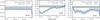 |
Fig. 2 Radial distribution of abundances with error-bars of CO, CN, and CS at the time of 104 yr. The RATRAN-derived values (dashed lines) are compared with the results of the best-fit 1D chemical model (solid lines); see Table 4 for the specifications. |
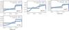 |
Fig. 3 As Fig. 2, for species with a jump at 100 K (lower inner abundance). |
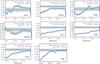 |
Fig. 4 As Fig. 2, for species with a constant abundance, based on only a few observed transitions. |
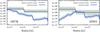 |
Fig. 5 As Fig. 2, for species with a jump at 230 K (higher inner abundance). |
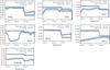 |
Fig. 6 As Fig. 2, for species with a jump at 100 K (higher inner abundance). |
4. Chemical structure of the protostellar envelope
With the 1D physical structure and chemical model described above, we calculated about 20 different realizations of the AFGL 2591 envelope by varying the initial elemental abundances, chemical ages, grain sizes, UV intensities, and cosmic ray ionization rates.
We identified several models that fit the RATRAN-based observational 1D abundance profiles reasonably well. Our best-fit model is based on the lm initial molecular abundances (with solar C/O ratio of 0.44; see Table 3), has a CR ionization rate of 5 × 10-17 s-1, an external UV intensity of one Draine interstellar UV field, and a chemical age of 10 − 50 kyr. The model is compared with a RATRAN-derived observed values in Figs. 2−6. The overall agreement between the observed and best-fit 1D abundance profiles is summarized in Table 4.
As one can clearly see from Table 4, more than 70% of the 1D RATRAN abundance profiles are reproduced within the uncertainties. The best fitted species are ortho- and para-H2, CO, HCO+, H2CO, CN, N2H+, NO, OH, OCS, H2CS, O, NH3, SO, H2O, and HNC. Species whose abundances in the 1D model are similar to the observationally derived values at some radii, but overall agreement is less clear are C, C+, CH, CCH, CS, SO2, H2S, and HCl (Figs. 2−6). Species whose 1D abundances are not fitted include HCN and CH3OH. Remarkably, many simplistic constant or jump-like 1D abundance profiles utilized in the RATRAN modeling of the observed lines correspond closely to the results of the rigorous 1D time-dependent chemical model.
Agreement (A) between the observed and best-fit 1D abundance profiles.
4.1. Photostable species located in the outflow cavity
Where the modeled abundance profiles for CCH, C, C+, CH, CS, SO2, and HCl coincide with the respective RATRAN profiles at some radii, the HCN and CH3OH abundances in the best-fit model are lower than the RATRAN-derived values. The first reason for this disagreement is a fundamental restriction of the utilized 1D approach with which one cannot properly capture the physical and chemical processes that occur on the walls of UV-irradiated outflow cavity. The presence of the outflow cavity and even a disk-like rotating structure in the AFGL 2591 is well established (see, e.g., Tamura & Yamashita 1992; Bruderer et al. 2010b; Wang et al. 2012). Clearly, in this case such a complex environment is better characterized by a 2D or even 3D model.
As shown by Bruderer et al. (2010b), a multidimensional approach is required to explain the observed abundances of light hydrides and hydride ions, such as OH+. As we do not include a central UV source in our model (since its radiation in the 1D approach is quickly absorbed by the massive envelope inner regions), our model tends to under-predict the abundances of simple photostable radicals and PDR-like species. This may explain why the abundances of species like C, C+, CH, CN, CCH, and HCl at small radii (≲1014 m) are lower in the model than the RATRAN-derived observed values. For HCl, which has a very limited chemistry network in our model of only 58 channels, the lack of major high-temperature production channels may also play a role.
We increased the external UV intensity by factors of 50 and 500 compared to the best-fit model, but found that is has no effect on the calculated abundances because the enhanced interstellar UV field cannot penetrate deeply into the massive AFGL 2591 envelope and the resulting UV-irradiated volume is negligible in the 1D spherically-symmetric case, unlike in the 2D model with the outflow (e.g., as described in Bruderer et al. 2010b).
Thus, the 1D approach that is often employed to model and understand the chemical composition of low- and high-mass protostellar objects appears inappropriate for PDR-like ions and molecules. To explain their elevated abundances, a 2D or 3D model with a detailed description of the outflow physics (central X-ray or FUV source irradiating outflow cavity walls, outflow-induced shocks at the walls, etc.) must be utilized.
4.2. HCN and HNC
Our models are able to fit either the HCN or the HNC abundance, but not both. This discrepancy reflects the limitations of modern astrochemical models that are not capable of explaining why the observed HNC/HCN abundance ratio decreases with increasing temperature in regions of low- and high-mass star formation (see recent discussion in Graninger et al. 2014). One explanation is that the energy barrier of the isomerization reaction converting HNC to HCN by collisions with atomic H, quantum-chemically calculated to be ~1200 K, should in fact be lower, ~200 K. Alternatively, a high-temperature destruction channel of HNC may be missing in the models, and one option is the reaction of HNC with O. The KIDA database gives a rate constant of ~10-12 cm3 s-1 and a barrier of >1000 K, which would suggest that this reaction only plays a minor role in the AFGL 2591 envelope. However, the reaction data are uncertain and we recommend an accurate measurement of this potentially important reaction. Third, the dynamical and thermal evolution of the environment may play a significant role in the HCN/HNC isomer-specific formation and destruction chemistry; our model does not consider this effect as it is based on a static physical structure of the AFGL 2591 envelope.
4.3. Complex organics
The problem with predicting CH3OH abundances is that this species is produced as ice on dust grain surfaces during the cold, pre-AFGL 2591 phase and is later injected into the gas phase as a result of heating. Because our 1D model does not include a warm-up phase, but rather a simple two-stage cold-to-warm jump-like evolution, it probably does not allow methanol precursor ices to be sufficiently accumulated in grain mantles (see Garrod et al. 2008). In addition, we model the pre-AFGL phase assuming 0D physical conditions, which may not be sufficient for the 1D model used after that. It might also be that our approach to model CO hydrogenation on the dust surfaces does not include all the necessary details such as a multi-phase ice structure (chemically inert, bulk ice with chemically active ice layers), porosity, and the presence of surface binding sites of different energies (see Taquet et al. 2012; Vasyunin & Herbst 2013a,b; Garrod 2013). This deficiency can be best demonstrated by the recent puzzling detections of complex organic molecules in cold, pre-stellar cores and infrared dark clouds, which is a challenge to explain without too much tuning of the key chemistry parameters such as reactive desorption efficiency, probabilities of radiative association between large molecules, and their least-destructive dissociative recombination (e.g., Bacmann et al. 2012; Vasyunin & Herbst 2013b; Vasyunina et al. 2014; Öberg et al. 2014). Interestingly, with our other models with elemental C/O ratios > 1 we can accurately reproduce the entire 1D RATRAN CH3OH profile, but then the H2CO abundances in these models become too high.
4.4. S-bearing species
Another problem with many contemporary astrochemical models is simultaneously explaining the observed abundances of simple S-bearing species like CS and more complex species such as SO, SO2, and OCS, and predicting the main reservoir of sulfur. The problem is particularly acute in protoplanetary disk chemistry (Dutrey et al. 2011) and high-mass star-forming regions (e.g., Wakelam et al. 2011). The reasons are a lack of data on sulfur chemistry from laboratory experiments and quantum chemistry simulations (Wakelam et al. 2010), and omission of key S-bearing complex species in the networks (see Druard & Wakelam 2012). Another explanation is the lack of X-ray-driven chemistry in our model, which can be important for the evolution of S-bearing species in high-mass star-forming regions (see Stäuber et al. 2005; Benz et al. 2007).
Recently, Esplugues et al. (2014) have performed extensive chemo-dynamical modeling of the sulfur chemistry in Orion KL with the UCL_CHEM chemical code and two different evolutionary phases. In Phase I, depletion of atoms and molecules onto dust grain surfaces begins in a collapsing prestellar core. In Phase II, a protostar is formed and steadily heats the surrounding medium, evaporating the ices back into the gas phase. With this time-dependent physical and chemical model, Esplugues et al. (2014) were able to simultaneously reproduce the observed column densities of SO, SO2, CS, OCS, H2S, and H2CS, assuming an initial S abundance of 10% of the solar value and a density ≳ 5 × 106 cm-3.
In our models, only 1% of cosmic sulfur is available for gaseous and surface chemistry, while the rest is locked in solid form. In the standard lm model, the main reservoirs of gas-phase sulfur are SO and SO2, with H2CS an important reservoir only at T> 700 K. In the other two models with C/O > 1, CS-bearing species, especially CS and H2CS, become the dominant S-bearing species, while the importance of SO and SO2 decreases.
Our best-fit chemical model does reproduce reasonably well all the observed and analyzed S-bearing molecules in AFGL 2591 (CS, OCS, SO, SO2, H2CS, and H2S; see Figs. 2−6). Only SO2 and H2S are not well fitted in the inner region at r ≲ 5 × 10¹⁴ m-2 (Fig. 5). The 1D modeled profile is almost constant for SO2 and does not show a jump-like decrease at T = 100 K, as is found with the detailed RATRAN modeling. Still, the difference between the values calculated with the chemical and RATRAN models is almost within the computational uncertainties. The situation is more severe for H2S, where the 1D chemical model shows an abundance decrease of almost 8 orders of magnitude at r ~ 3 × 10¹⁴ m, where neutral-neutral reactions with O and OH start destroying H2S at T> 140 − 200 K. This jump-like behavior is not seen in the RATRAN models, which may be due to our neglect of enhanced UV irradiation of the outflow cavity walls and inner envelope regions, which facilitate the formation of rich, heavy ices and their desorption into the gas phase.
Sensitivity of assorted molecules to varied parameters of the model, the ionization rate (CR), the C/O ratio, and the chemical age.
4.5. Other good models
In addition to our best-fit lm model with an age of 10 − 50 kyr and a solar elemental C/O ratio of 0.4, we identified two other good models with h11 initial abundances with an elemental C/O ratio of 1.13 (see Table 3) and ages of 10 and 50 kyr. Unlike the standard model, with these two models the agreement is much better between the chemical and RATRAN-derived abundances of CH3OH, HCN, HNC, CH, and CCH. However, these two models fail to reproduce the abundances of important species such as CO, HCO+, H2CO, and CN.
The first reason is that the initial molecular abundances in the two C/O > 1 models are calculated assuming a warmer T = 15 K than the T = 10 K in the lm model. The higher temperature leads to faster diffusion rates for atomic hydrogen and hence more efficient hydrogenation of CO ice into H2CO and CH3OH ice. As a result, the abundances of gaseous H2CO and CH3OH become higher and are in better agreement with the observed values than with the standard lm model.
The second reason is the excess of elemental carbon that remains available after almost all elemental oxygen is locked in CO and CO2. This carbon goes into production of various hydrocarbons and cyanopolyynes (Table 3), making HCN, HNC, CH, and CCH more abundant and better fitted than with the lm solar C/O model.
4.6. Influence of different parameters on chemical abundances
The overall sensitivity of the modeled molecules to variations of the physical and chemical parameters of the 1D model is summarized in Table 5.
First, we find that the modeling results are not sensitive to the adopted value of the average grain size. This is not surprising because the envelope is warmer than 30 K and has a rather low age of around 1 − 5 × 10⁴ years. Under such conditions the ices that were produced in the earlier, colder pre-AFGL 2591 phase have mostly evaporated and surface processing becomes of minor importance for the global chemical evolution of the envelope.
The same is true for two other models where the external UV intensity was 50 and 500 (in Draine’s interstellar UV units) compared to the best-fit model with 1 Draine UV field. As we stated above, this is because the external UV field cannot penetrate deeply into the massive, dense AFGL 2591 envelope, and the corresponding propagation of the PDR-like outer shell inward is negligible.
4.6.1. Ionization rate
The species that are sensitive to the enhanced CR ionization rate values of 5 × 10-16 s-1 and 5 × 10-15 s-1 include H2O, molecular ions like HCO+ or N2H+, and organics such as H2CO and H2CS. Because of the higher ionization in these models, the modeled abundances of ions are over-predicted compared to the best-fit model and the RATRAN-derived values, whereas abundances of water and the organic species are under-predicted. The rest of the considered molecules are not very sensitive to the adopted CR ionization rate.
4.6.2. C/O ratio
Most of the species in Table 5 are sensitive to the adopted initial abundances and the C/O ratio. The only exceptions are several simple H- and N-bearing species (H2, N2H+), C and C+, and HCl. Both C and C+ are abundant in the outer, UV-irradiated part of the envelope, where they are the dominant carbon-based species. Consequently, their abundances differ by only a factor of about 2 between the lm and d11c and h11 models (see Table 2). The abundances of HCl, and also of H2 and N2H+, are not sensitive to the C/O ratio because their major formation and destruction pathways do not include reactions with C- or O-bearing species.
4.6.3. Chemical age
Molecules whose 1D abundance profiles are affected by the chemical age are mostly heavy S-bearing and N-bearing species, namely, H2CS, OCS, NH3, H2S; and HCN and HNC (Table 5). Less sensitive to the chemical age are the abundances of H2CO, CH, and CS. As established more than two decades ago by e.g., Suzuki et al. (1992), abundance ratios of sulfur- and nitrogen-bearing species such as CCS/NH3 can be employed as chemical age estimators in cold pre-stellar cores, because sulfur-bearing species like CCS are formed rather rapidly via gas-phase chemistry involving hydrocarbons (CH, CCH, etc.), whereas nitrogen chemistry takes longer to convert N to N2 and to other N-bearing species like HCN and HNC. Naturally, characteristic chemical timescales of NH3, which is mainly formed on dust grain surfaces, are rather long (> 105 years in molecular clouds). This is also true for other complex species produced via surface chemistry, like H2CO, H2CS, and CH3OH. As we discussed above, the best-fit models for the AFGL 2591 1D chemical structure are those with short chemical ages of 10 − 50 kyr, which is similar to the derived age of the AFGL 2591 of ~ 50 kyr (Doty et al. 2002).
5. Conclusions
Based on HIFI and JCMT observations we derived molecular abundances of about 25 species detected in the protostellar envelope of AFGL 2591. Two methods were applied to interpret the data. First, detailed radiative transfer calculations with RATRAN were performed, using an adequate 1D physical model of the envelope. Then, abundances were calculated with time-dependent chemical models with varied cosmic ray ionization rates, external UV intensities, grain sizes, ages, and initial molecular abundances based on various C/O elemental abundances. By comparing the results from these two methods, we reach the following conclusions:
-
1.
The radial abundance profiles for 25 species were derived; i.e.,H2, CO, CN, CS, HCO+, H2CO, N2H+, CCH, NO, OCS, OH, H2CS, O,C, C+, CH, HCN, HNC, NH3, SO, SO2, H2S, H2O, HCl, and CH3OH.
-
2.
Based on radiative transfer calculations, three molecules (CO, CN, CS) were firmly fitted by a constant abundance model. The line fluxes of HCO+, H2CO, N2H+, and CCH can be fitted equally well by a constant abundance model and by a model with a jump at 100 K, with lower inner abundances. Species such as NO, OCS, OH, H2CS, O, C, C+, and CH were fitted by a constant abundance model; however, because of a lack of data, models with jumps cannot be excluded. The best model for HCN and HNC was with a jump at 230 K, with a higher inner abundance. The best model for molecules such as NH3, SO, SO2, H2S, H2O, HCl, and CH3OH was with a jump at 100 K, again with a higher inner abundance.
-
3.
The best time-dependent chemical model predicts a chemical age of AFGL 2591 of ~ 10 − 50 kyr, a solar C/O ratio of 0.44, and a cosmic ray ionization rate of ~ 5 × 10-17 s-1.
-
4.
Among our considered 25 species, the time-dependent chemical model can explain the abundance profiles of 15 of them within the errors. The remaining molecular abundances are affected by limited reaction networks (Cl- and S-bearing species), the lack of observed transitions (e.g., C, O, C+, and CH), or deficiencies of the surface chemistry model (CH3OH), which cause higher uncertainties and reduced agreement.
-
5.
We found that grain properties and intensity of the external UV field do not strongly affect the chemical structure of the AFGL 2591 envelope (at least with the adopted 1D geometry), whereas the chemical age, cosmic ray ionization rate, and initial abundances play an important role.
-
6.
Molecules that are sensitive to the presence of the outflow and UV/X-ray irradiation are C, C+, CH, CCH, CS, SO2, and other S-bearing molecules.
-
7.
Molecules that are sensitive to the cosmic ray ionization rate are H2O, molecular ions like HCO+, N2H+, and organic species such as H2CO and H2CS.
-
8.
Molecules that are sensitive to the adopted chemical age include heavy H2CS, OCS, NH3, H2S; HCN and HNC; and to a lesser degree H2CO, CH, and CS.
-
9.
The only molecules that are not sensitive to the initial molecular abundances and C/O ratios are simple H- and N-bearing species like H2, N2H+; C and C+; and HCl.
The main conclusion of this work is that simple constant or jump-like abundance profiles reproduce accurately single-dish submillimeter observations, and are supported by the predictions of a time-dependent gas-grain chemical model bound to a 1D physical structure. Future studies aimed at explaining the chemical structure of all observed species in the AFGL 2591 envelope should consider 2D or even 3D envelope geometry with an outflow cavity, and include the evolution of its temperature and density and, possibly, X-ray irradiation from the central source(s).
The James Clerk Maxwell Telescope is operated by the Joint Astronomy Centre on behalf of the Science and Technology Facilities Council of the United Kingdom, the Netherlands Organisation for Scientific Research, and the National Research Council of Canada.
SCUBA is a submillimeter continuum array receiver operated on the James Clerk Maxwell Telescope, on Mauna Kea, Hawaii.
PACS (Poglitsch et al. 2010) is the Photodetector Array Camera and Spectrometer onboard the ESA Herschel Space Observatory.
Acknowledgments
We thank Robert Barthel for his help with the calculations, Veronica Allen for useful suggestions, and an anonymous referee for a helpful report. D. Semenov acknowledges support by the Deutsche Forschungsgemeinschaft through SPP 1385: “The first ten million years of the solar system – a planetary materials approach” (SE 1962/1-3). HIFI has been designed and built by a consortium of institutes and university departments from across Europe, Canada and the United States under the leadership of SRON Netherlands Institute for Space Research, Groningen, The Netherlands and with major contributions from Germany, France and the US. Consortium members are: Canada: CSA, U. Waterloo; France: CESR, LAB, LERMA, IRAM; Germany: KOSMA, MPIfR, MPS; Ireland, NUI Maynooth; Italy: ASI, IFSI-INAF, Osservatorio Astrofisico di Arcetri-INAF; Netherlands: SRON, TUD; Poland: CAMK, CBK; Spain: Observatorio Astronómico Nacional (IGN), Centro de Astrobiologa (CSIC-INTA). Sweden: Chalmers University of Technology – MC2, RSS & GARD; Onsala Space Observatory; Swedish National Space Board, Stockholm University – Stockholm Observatory; Switzerland: ETH Zurich, FHNW; USA: Caltech, JPL, NHSC. This research made use of NASA’s Astrophysics Data System.
References
- Agúndez, M., & Wakelam, V. 2013, Chem. Rev., 113, 8710 [CrossRef] [PubMed] [Google Scholar]
- Albertsson, T., Semenov, D. A., Vasyunin, A. I., Henning, T., & Herbst, E. 2013, ApJS, 207, 27 [NASA ADS] [CrossRef] [Google Scholar]
- Albertsson, T., Semenov, D., & Henning, T. 2014, ApJ, 784, 39 [NASA ADS] [CrossRef] [Google Scholar]
- Bacmann, A., Taquet, V., Faure, A., Kahane, C., & Ceccarelli, C. 2012, A&A, 541, L12 [NASA ADS] [CrossRef] [EDP Sciences] [Google Scholar]
- Benz, A. O., Stäuber, P., Bourke, T. L., et al. 2007, A&A, 475, 549 [NASA ADS] [CrossRef] [EDP Sciences] [Google Scholar]
- Biham, O., Furman, I., Pirronello, V., & Vidali, G. 2001, ApJ, 553, 595 [NASA ADS] [CrossRef] [Google Scholar]
- Bisschop, S. E., Fraser, H. J., Öberg, K. I., van Dishoeck, E. F., & Schlemmer, S. 2006, A&A, 449, 1297 [NASA ADS] [CrossRef] [EDP Sciences] [Google Scholar]
- Boonman, A. M. S., Stark, R., van der Tak, F. F. S., et al. 2001, ApJ, 553, L63 [NASA ADS] [CrossRef] [Google Scholar]
- Bruderer, S., Benz, A. O., Doty, S. D., van Dishoeck, E. F., & Bourke, T. L. 2009a, ApJ, 700, 872 [NASA ADS] [CrossRef] [Google Scholar]
- Bruderer, S., Doty, S. D., & Benz, A. O. 2009b, ApJS, 183, 179 [NASA ADS] [CrossRef] [Google Scholar]
- Bruderer, S., Benz, A. O., Stäuber, P., & Doty, S. D. 2010a, ApJ, 720, 1432 [NASA ADS] [CrossRef] [Google Scholar]
- Bruderer, S., Benz, A. O., van Dishoeck, E. F., et al. 2010b, A&A, 521, L44 [NASA ADS] [CrossRef] [EDP Sciences] [Google Scholar]
- Ceccarelli, C., Bacmann, A., Boogert, A., et al. 2010, A&A, 521, L22 [NASA ADS] [CrossRef] [EDP Sciences] [Google Scholar]
- Cernicharo, J., Spielfiedel, A., Balança, C., et al. 2011, A&A, 531, A103 [NASA ADS] [CrossRef] [EDP Sciences] [Google Scholar]
- Choi, Y., van der Tak, F. F. S., van Dishoeck, E. F., Herpin, F., & Wyrowski, F., 2014, A&A, accepted [arXiv:1412.4818] [Google Scholar]
- Danby, G., Flower, D. R., Valiron, P., Schilke, P., & Walmsley, C. M. 1988, MNRAS, 235, 229 [NASA ADS] [CrossRef] [Google Scholar]
- Daniel, F., Dubernet, M.-L., & Grosjean, A. 2011, A&A, 536, A76 [NASA ADS] [CrossRef] [EDP Sciences] [Google Scholar]
- De Graauw, T., Helmich, F. P., Phillips, T. G., et al. 2010, A&A, 518, L6 [NASA ADS] [CrossRef] [EDP Sciences] [Google Scholar]
- Dobrijevic, M., Ollivier, J. L., Billebaud, F., Brillet, J., & Parisot, J. P. 2003, A&A, 398, 335 [NASA ADS] [CrossRef] [EDP Sciences] [Google Scholar]
- Doty, S. D., van Dishoeck, E. F., van der Tak, F. F. S., & Boonman, A. M. S. 2002, A&A, 389, 446 [NASA ADS] [CrossRef] [EDP Sciences] [Google Scholar]
- Draine, B. T. 1978, ApJ, 36, 595 [Google Scholar]
- Druard, C., & Wakelam, V. 2012, MNRAS, 426, 354 [NASA ADS] [CrossRef] [Google Scholar]
- Dubernet, M.-L., Daniel, F., Grosjean, A., et al. 2006, A&A, 460, 323 [NASA ADS] [CrossRef] [EDP Sciences] [Google Scholar]
- Dumouchel, F., Faure, A., & Lique, F. 2010, MNRAS, 406, 2488 [NASA ADS] [CrossRef] [Google Scholar]
- Dutrey, A., Wakelam, V., Boehler, Y., et al. 2011, A&A, 535, A104 [NASA ADS] [CrossRef] [EDP Sciences] [Google Scholar]
- Esplugues, G. B., Viti, S., Goicoechea, J. R., & Cernicharo, J. 2014, A&A, 567, A95 [NASA ADS] [CrossRef] [EDP Sciences] [Google Scholar]
- Fayolle, E. C., Bertin, M., Romanzin, C., et al. 2011a, ApJ, 739, L36 [NASA ADS] [CrossRef] [Google Scholar]
- Fayolle, E. C., Öberg, K. I., Cuppen, H. M., Visser, R., & Linnartz, H. 2011b, A&A, 529, A74 [NASA ADS] [CrossRef] [EDP Sciences] [Google Scholar]
- Fayolle, E. C., Bertin, M., Romanzin, C., et al. 2013, A&A, 556, A122 [NASA ADS] [CrossRef] [EDP Sciences] [Google Scholar]
- Flower, D. 1990, Molecular collisions in the interstellar medium (Cambridge: University Press) [Google Scholar]
- Flower, D. R. 1999, MNRAS, 305, 651 [NASA ADS] [CrossRef] [Google Scholar]
- Flower, D. R. 2001, MNRAS, 328, 147 [Google Scholar]
- Flower, D. R., & Launay, J. M. 1977, J. Phys. B Atom. Mol. Phys., 10, 3673 [NASA ADS] [CrossRef] [Google Scholar]
- Flower, D. R., Pineau des Forêts, G., & Walmsley, C. M. 2004, A&A, 427, 887 [NASA ADS] [CrossRef] [EDP Sciences] [Google Scholar]
- Flower, D. R., Pineau Des Forêts, G., & Walmsley, C. M. 2006, A&A, 449, 621 [NASA ADS] [CrossRef] [EDP Sciences] [Google Scholar]
- Garrod, R. T. 2013, ApJ, 778, 158 [NASA ADS] [CrossRef] [Google Scholar]
- Garrod, R. T., & Herbst, E. 2006, A&A, 457, 927 [NASA ADS] [CrossRef] [EDP Sciences] [Google Scholar]
- Garrod, R. T., Wakelam, V., & Herbst, E. 2007, A&A, 467, 1103 [NASA ADS] [CrossRef] [EDP Sciences] [Google Scholar]
- Garrod, R. T., Weaver, S. L. W., & Herbst, E. 2008, ApJ, 682, 283 [NASA ADS] [CrossRef] [Google Scholar]
- Gerlich, D. 1990, J. Chem. Phys., 92, 2377 [NASA ADS] [CrossRef] [Google Scholar]
- Gerlich, D., Herbst, E., & Roueff, E. 2002, Planet. Space Sci., 50, 1275 [NASA ADS] [CrossRef] [Google Scholar]
- Graedel, T. E., Langer, W. D., & Frerking, M. A. 1982, ApJS, 48, 321 [NASA ADS] [CrossRef] [Google Scholar]
- Graninger, D. M., Herbst, E., Öberg, K. I., & Vasyunin, A. I. 2014, ApJ, 787, 74 [NASA ADS] [CrossRef] [Google Scholar]
- Green, S. 1995, ApJS, 100, 213 [NASA ADS] [CrossRef] [Google Scholar]
- Green, S., & Chapman, S. 1978, ApJS, 37, 169 [NASA ADS] [CrossRef] [Google Scholar]
- Harada, N., Herbst, E., & Wakelam, V. 2010, ApJ, 721, 1570 [NASA ADS] [CrossRef] [Google Scholar]
- Harada, N., Herbst, E., & Wakelam, V. 2012, ApJ, 756, 104 [NASA ADS] [CrossRef] [Google Scholar]
- Hasegawa, T. I., Herbst, E., & Leung, C. M. 1992, ApJS, 82, 167 [NASA ADS] [CrossRef] [Google Scholar]
- Herbst, E., & van Dishoeck, E. F. 2009, ARA&A, 47, 427 [NASA ADS] [CrossRef] [Google Scholar]
- Herpin, F., Chavarría, L., van der Tak, F., et al. 2012, A&A, 542, A76 [NASA ADS] [CrossRef] [EDP Sciences] [Google Scholar]
- Hincelin, U., Wakelam, V., Hersant, F., et al. 2011, A&A, 530, A61 [NASA ADS] [CrossRef] [EDP Sciences] [Google Scholar]
- Hogerheijde, M. R., & van der Tak, F. F. S. 2000, A&A, 362, 697 [NASA ADS] [Google Scholar]
- Honvault, P., Jorfi, M., González-Lezana, T., Faure, A., & Pagani, L. 2011, Phys. Rev. Lett., 107, 023201 [NASA ADS] [CrossRef] [Google Scholar]
- Hugo, E., Asvany, O., & Schlemmer, S. 2009, J. Chem. Phys., 130, 164302 [NASA ADS] [CrossRef] [PubMed] [Google Scholar]
- Jaquet, R., Staemmler, V., Smith, M. D., & Flower, D. R. 1992, J. Phys. B Atom. Mol. Phys., 25, 285 [Google Scholar]
- Jiménez-Serra, I., Zhang, Q., Viti, S., Martín-Pintado, J., & de Wit, W.-J. 2012a, ApJ, 753, 34 [NASA ADS] [CrossRef] [Google Scholar]
- Jiménez-Serra, I., Zhang, Q., Viti, S., Martín-Pintado, J., & de Wit, W.-J. 2012b, ApJ, 753, 34 [NASA ADS] [CrossRef] [Google Scholar]
- Johnston, K. G., Shepherd, D. S., Robitaille, T. P., & Wood, K. 2013, A&A, 551, A43 [NASA ADS] [CrossRef] [EDP Sciences] [Google Scholar]
- Jørgensen, J. K., Schöier, F. L., & van Dishoeck, E. F. 2004, A&A, 416, 603 [NASA ADS] [CrossRef] [EDP Sciences] [Google Scholar]
- Katz, N., Furman, I., Biham, O., Pirronello, V., & Vidali, G. 1999, ApJ, 522, 305 [NASA ADS] [CrossRef] [Google Scholar]
- Kaźmierczak-Barthel, M., van der Tak, F. F. S., Helmich, F. P., et al. 2014, A&A, 567, A53 [NASA ADS] [CrossRef] [EDP Sciences] [Google Scholar]
- Lee, H.-H., Roueff, E., Pineau des Forets, G., et al. 1998, A&A, 334, 1047 [NASA ADS] [Google Scholar]
- Lique, F., Dubernet, M.-L., Spielfiedel, A., & Feautrier, N. 2006a, A&A, 450, 399 [NASA ADS] [CrossRef] [EDP Sciences] [Google Scholar]
- Lique, F., Spielfiedel, A., & Cernicharo, J. 2006b, A&A, 451, 1125 [NASA ADS] [CrossRef] [EDP Sciences] [Google Scholar]
- Lique, F., van der Tak, F. F. S., Kłos, J., Bulthuis, J., & Alexander, M. H. 2009, A&A, 493, 557 [NASA ADS] [CrossRef] [EDP Sciences] [Google Scholar]
- Lique, F., Spielfiedel, A., Feautrier, N., et al. 2010, J. Chem. Phys., 132, 024303 [NASA ADS] [CrossRef] [PubMed] [Google Scholar]
- Loison, J.-C., Halvick, P., Bergeat, A., Hickson, K. M., & Wakelam, V. 2012, MNRAS, 421, 1476 [NASA ADS] [CrossRef] [Google Scholar]
- Maret, S., Faure, A., Scifoni, E., & Wiesenfeld, L. 2009, MNRAS, 399, 425 [NASA ADS] [CrossRef] [Google Scholar]
- Neufeld, D. A., & Green, S. 1994, ApJ, 432, 158 [NASA ADS] [CrossRef] [Google Scholar]
- Öberg, K. I., Garrod, R. T., van Dishoeck, E. F., & Linnartz, H. 2009a, A&A, 504, 891 [NASA ADS] [CrossRef] [EDP Sciences] [Google Scholar]
- Öberg, K. I., van Dishoeck, E. F., & Linnartz, H. 2009b, A&A, 496, 281 [NASA ADS] [CrossRef] [EDP Sciences] [Google Scholar]
- Öberg, K. I., Lauck, T., & Graninger, D. 2014, ApJ, 788, 68 [NASA ADS] [CrossRef] [Google Scholar]
- Offer, A. R., van Hemert, M. C., & van Dishoeck, E. F. 1994, J. Chem. Phys., 100, 362 [NASA ADS] [CrossRef] [Google Scholar]
- Pagani, L., Vastel, C., Hugo, E., et al. 2009, A&A, 494, 623 [NASA ADS] [CrossRef] [EDP Sciences] [Google Scholar]
- Pilbratt, G. L., Riedinger, J. R., Passvogel, T., et al. 2010, A&A, 518, L1 [CrossRef] [EDP Sciences] [Google Scholar]
- Plume, R., Fuller, G. A., Helmich, F., et al. 2007, PASP, 119, 102 [NASA ADS] [CrossRef] [Google Scholar]
- Poglitsch, A., Waelkens, C., Geis, N., et al. 2010, A&A, 518, L2 [NASA ADS] [CrossRef] [EDP Sciences] [Google Scholar]
- Rabli, D., & Flower, D. R. 2010, MNRAS, 406, 95 [NASA ADS] [CrossRef] [Google Scholar]
- Roberts, H., & Millar, T. J. 2000, A&A, 361, 388 [NASA ADS] [Google Scholar]
- Roberts, H., Herbst, E., & Millar, T. J. 2004, A&A, 424, 905 [NASA ADS] [CrossRef] [EDP Sciences] [Google Scholar]
- Rodgers, S. D., & Charnley, S. B. 2001, ApJ, 546, 324 [Google Scholar]
- Roueff, E. 1990, Collisional excitation processes (Cambridge: University Press), 232 [Google Scholar]
- Ruffle, D. P., & Herbst, E. 2000, MNRAS, 319, 837 [NASA ADS] [CrossRef] [Google Scholar]
- Roueff, E., & Lique, F. 2013, Chem. Rev., 113, 8906 [CrossRef] [PubMed] [Google Scholar]
- Roueff, E., Lis, D. C., van der Tak, F. F. S., Gerin, M., & Goldsmith, P. F. 2005, A&A, 438, 585 [NASA ADS] [CrossRef] [EDP Sciences] [Google Scholar]
- Rygl, K. L. J., Brunthaler, A., Sanna, A., et al. 2012, A&A, 539, A79 [NASA ADS] [CrossRef] [EDP Sciences] [Google Scholar]
- Sanna, A., Reid, M. J., Carrasco-González, C., et al. 2012, ApJ, 745, 191 [NASA ADS] [CrossRef] [Google Scholar]
- Schöier, F. L., Jørgensen, J. K., van Dishoeck, E. F., & Blake, G. A. 2002, A&A, 390, 1001 [NASA ADS] [CrossRef] [EDP Sciences] [Google Scholar]
- Schöier, F. L., van der Tak, F. F. S., van Dishoeck, E. F., & Black, J. H. 2005, A&A, 432, 369 [NASA ADS] [CrossRef] [EDP Sciences] [Google Scholar]
- Schröder, K., Staemmler, V., Smith, M. D., Flower, D. R., & Jaquet, R. 1991, J. Phys. B Atom. Mol. Phys., 24, 2487 [CrossRef] [Google Scholar]
- Semenov, D., & Wiebe, D. 2011, ApJ, 196, 25 [Google Scholar]
- Semenov, D., Hersant, F., Wakelam, V., et al. 2010, A&A, 522, A42 [NASA ADS] [CrossRef] [EDP Sciences] [Google Scholar]
- Sipilä, O., Caselli, P., & Harju, J. 2013, A&A, 554, A92 [NASA ADS] [CrossRef] [EDP Sciences] [Google Scholar]
- Spielfiedel, A., Feautrier, N., Najar, F., et al. 2012, MNRAS, 421, 1891 [NASA ADS] [CrossRef] [Google Scholar]
- Stäuber, P., Doty, S. D., van Dishoeck, E. F., Jørgensen, J. K., & Benz, A. O. 2004, A&A, 425, 577 [NASA ADS] [CrossRef] [EDP Sciences] [Google Scholar]
- Stäuber, P., Doty, S. D., van Dishoeck, E. F., & Benz, A. O. 2005, A&A, 440, 949 [NASA ADS] [CrossRef] [EDP Sciences] [Google Scholar]
- Stäuber, P., Benz, A. O., Jørgensen, J. K., et al. 2007, A&A, 466, 977 [NASA ADS] [CrossRef] [EDP Sciences] [Google Scholar]
- Suzuki, H., Yamamoto, S., Ohishi, M., et al. 1992, ApJ, 392, 551 [NASA ADS] [CrossRef] [Google Scholar]
- Takano, T., Stutzki, J., Winnewisser, G., & Fukui, Y. 1986, A&A, 158, 14 [NASA ADS] [Google Scholar]
- Tamura, M., & Yamashita, T. 1992, ApJ, 391, 710 [NASA ADS] [CrossRef] [Google Scholar]
- Tan, J. C., Beltran, M. T., Caselli, P., et al. 2014, Protostars and Planets VI, eds. H. Beuther, R. Klessen, C. Dullemond, & Th. Henning (University of Arizona Press), in press [arXiv:1402.0919] [Google Scholar]
- Taquet, V., Ceccarelli, C., & Kahane, C. 2012, A&A, 538, A42 [NASA ADS] [CrossRef] [EDP Sciences] [Google Scholar]
- Trinidad, M. A., Curiel, S., Cantó, J., et al. 2003, ApJ, 589, 386 [NASA ADS] [CrossRef] [Google Scholar]
- van der Tak, F. 2011, in IAU Symp. 280, eds. J. Cernicharo, & R. Bachiller, 449 [Google Scholar]
- van der Tak, F. F. S., & Menten, K. M. 2005, A&A, 437, 947 [NASA ADS] [CrossRef] [EDP Sciences] [Google Scholar]
- van der Tak, F. F. S., & Van Dishoeck, E. F. 2000, A&A, 358, L79 [NASA ADS] [Google Scholar]
- van der Tak, F. F. S., van Dishoeck, E. F., Evans, II, N. J., Bakker, E. J., & Blake, G. A. 1999, ApJ, 522, 991 [NASA ADS] [CrossRef] [Google Scholar]
- van der Tak, F. F. S., van Dishoeck, E. F., & Caselli, P. 2000a, A&A, 361, 327 [NASA ADS] [Google Scholar]
- van der Tak, F. F. S., van Dishoeck, E. F., Evans, II, N. J., & Blake, G. A. 2000b, ApJ, 537, 283 [NASA ADS] [CrossRef] [Google Scholar]
- van der Tak, F. F. S., Boonman, A. M. S., Braakman, R., & van Dishoeck, E. F. 2003, A&A, 412, 133 [NASA ADS] [CrossRef] [EDP Sciences] [Google Scholar]
- van der Tak, F. F. S., Walmsley, C. M., Herpin, F., & Ceccarelli, C. 2006, A&A, 447, 1011 [NASA ADS] [CrossRef] [EDP Sciences] [Google Scholar]
- van der Tak, F. F. S., Chavarría, L., Herpin, F., et al. 2013, A&A, 554, A83 [NASA ADS] [CrossRef] [EDP Sciences] [Google Scholar]
- van der Wiel, M. H. D., van der Tak, F. F. S., Spaans, M., et al. 2011, A&A, 532, A88 [NASA ADS] [CrossRef] [EDP Sciences] [Google Scholar]
- van der Wiel, M. H. D., Pagani, L., van der Tak, F. F. S., Kaźmierczak, M., & Ceccarelli, C. 2013, A&A, 553, A11 [NASA ADS] [CrossRef] [EDP Sciences] [Google Scholar]
- Van Dishoeck, E. F., & Blake, G. A. 1998, ARA&A, 36, 317 [NASA ADS] [CrossRef] [Google Scholar]
- Van Dishoeck, E. F., Jonkheid, B., & van Hemert, M. C. 2006, Faraday discussion, Photoprocesses in protoplanetary disks (Cambridge: Royal Society of Chemistry), 231 [Google Scholar]
- Vasyunin, A. I., & Herbst, E. 2013a, ApJ, 762, 86 [NASA ADS] [CrossRef] [Google Scholar]
- Vasyunin, A. I., & Herbst, E. 2013b, ApJ, 769, 34 [Google Scholar]
- Vasyunin, A. I., Sobolev, A. M., Wiebe, D. S., & Semenov, D. A. 2004, Astron. Lett., 30, 566 [NASA ADS] [CrossRef] [Google Scholar]
- Vasyunin, A. I., Semenov, D., Henning, T., et al. 2008, ApJ, 672, 629 [NASA ADS] [CrossRef] [Google Scholar]
- Vasyunina, T., Vasyunin, A. I., Herbst, E., et al. 2014, ApJ, 780, 85 [NASA ADS] [CrossRef] [Google Scholar]
- Veach, T. J., Groppi, C. E., & Hedden, A. 2013, ApJ, 765, L34 [NASA ADS] [CrossRef] [Google Scholar]
- Wakelam, V., Selsis, F., Herbst, E., & Caselli, P. 2005, A&A, 444, 883 [NASA ADS] [CrossRef] [EDP Sciences] [Google Scholar]
- Wakelam, V., Herbst, E., & Selsis, F. 2006, A&A, 451, 551 [NASA ADS] [CrossRef] [EDP Sciences] [Google Scholar]
- Wakelam, V., Smith, I. W. M., Herbst, E., et al. 2010, Space Sci. Rev., 156, 13 [NASA ADS] [CrossRef] [Google Scholar]
- Wakelam, V., Hersant, F., & Herpin, F. 2011, A&A, 529, A112 [NASA ADS] [CrossRef] [EDP Sciences] [Google Scholar]
- Wakelam, V., Herbst, E., Loison, J.-C., et al. 2012, ApJS, 199, 21 [NASA ADS] [CrossRef] [Google Scholar]
- Walmsley, C. M., Flower, D. R., & Pineau des Forêts, G. 2004, A&A, 418, 1035 [NASA ADS] [CrossRef] [EDP Sciences] [Google Scholar]
- Wang, K.-S., van der Tak, F. F. S., & Hogerheijde, M. R. 2012, A&A, 543, A22 [NASA ADS] [CrossRef] [EDP Sciences] [Google Scholar]
- Wiesenfeld, L., & Faure, A. 2013, MNRAS, 432, 2573 [NASA ADS] [CrossRef] [Google Scholar]
- Wilson, T. L., & Rood, R. 1994, ARA&A, 32, 191 [NASA ADS] [CrossRef] [Google Scholar]
- Yang, B., Stancil, P. C., Balakrishnan, N., & Forrey, R. C. 2010, ApJ, 718, 1062 [NASA ADS] [CrossRef] [Google Scholar]
- Zinnecker, H., & Yorke, H. W. 2007, ARA&A, 45, 481 [NASA ADS] [CrossRef] [Google Scholar]
All Tables
Abundances (relative to H2) estimated with the spherical radiative transfer model (RATRAN) for the envelope of AFGL 2591, based on HIFI and JCMT data.
Initial abundances (relative to total H) for modeling pre-AFGL 2591 evolutionary phase.
Top 25 of the initially abundant molecules (relative to total H) for the AFGL 2591 chemical modeling.
Sensitivity of assorted molecules to varied parameters of the model, the ionization rate (CR), the C/O ratio, and the chemical age.
All Figures
|
Fig. 1 Temperature and density structure of the 1D physical model of AFGL 2591. |
| In the text | |
|
Fig. 2 Radial distribution of abundances with error-bars of CO, CN, and CS at the time of 104 yr. The RATRAN-derived values (dashed lines) are compared with the results of the best-fit 1D chemical model (solid lines); see Table 4 for the specifications. |
| In the text | |
|
Fig. 3 As Fig. 2, for species with a jump at 100 K (lower inner abundance). |
| In the text | |
|
Fig. 4 As Fig. 2, for species with a constant abundance, based on only a few observed transitions. |
| In the text | |
|
Fig. 5 As Fig. 2, for species with a jump at 230 K (higher inner abundance). |
| In the text | |
|
Fig. 6 As Fig. 2, for species with a jump at 100 K (higher inner abundance). |
| In the text | |
Current usage metrics show cumulative count of Article Views (full-text article views including HTML views, PDF and ePub downloads, according to the available data) and Abstracts Views on Vision4Press platform.
Data correspond to usage on the plateform after 2015. The current usage metrics is available 48-96 hours after online publication and is updated daily on week days.
Initial download of the metrics may take a while.