| Issue |
A&A
Volume 574, February 2015
|
|
|---|---|---|
| Article Number | A67 | |
| Number of page(s) | 14 | |
| Section | Numerical methods and codes | |
| DOI | https://doi.org/10.1051/0004-6361/201424566 | |
| Published online | 27 January 2015 | |
Wavelet-based decomposition and analysis of structural patterns in astronomical images
1
Max-Planck-Institut für Radioastronomie,
Auf dem Hugel 69,
53121
Bonn,
Germany
e-mail:
florent.mertens@gmail.com
2
Institut für Experimentalphysik, Universität
Hamburg, Luruper Chaussee
149, 22761
Hamburg,
Germany
Received: 9 July 2014
Accepted: 28 November 2014
Context. Images of spatially resolved astrophysical objects contain a wealth of morphological and dynamical information, and effectively extracting this information is of paramount importance for understanding the physics and evolution of these objects. The algorithms and methods currently employed for this purpose (such as Gaussian model fitting) often use simplified approaches to describe the structure of resolved objects.
Aims. Automated (unsupervised) methods for structure decomposition and tracking of structural patterns are needed for this purpose to be able to treat the complexity of structure and large amounts of data involved.
Methods. We developed a new wavelet-based image segmentation and evaluation (WISE) method for multiscale decomposition, segmentation, and tracking of structural patterns in astronomical images.
Results. The method was tested against simulated images of relativistic jets and applied to data from long-term monitoring of parsec-scale radio jets in 3C 273 and 3C 120. Working at its coarsest resolution, WISE reproduces the previous results of a model-fitting evaluation of the structure and kinematics in these jets exceptionally well. Extending the WISE structure analysis to fine scales provides the first robust measurements of two-dimensional velocity fields in these jets and indicates that the velocity fields probably reflect the evolution of Kelvin-Helmholtz instabilities that develop in the flow.
Key words: methods: data analysis / galaxies: jets / galaxies: groups: individual: 3C 120 / quasars: individual: 3C 273
© ESO, 2015
1. Introduction
The steady improvements of the dynamic range of astronomical images and the ever-increasing complexity and detail of astrophysical modeling bring a higher demand on automatic (or unsupervised) methods for characterizing and analyzing structural patterns in astronomical images.
Several of the approaches developed in the fields of computer vision and remote- sensing to track structural changes (cf. Yuan et al. 1998; Doucet & Gordon 1999; Arulampalam et al. 2002; Sidenbladh et al. 2004; Doucet & Wang 2005; Myint et al. 2008) either require oversampling in the temporal domain or rely on multiband (multicolor) information that underlies the changing patterns. This renders them difficult to be used in astronomical applications that typically focus on tracking changes in brightness in a single observing band, which are monitored with sparse sampling, and in which the structural displacements between individual image frames often exceed the dimensions of the instrumental point spread function (PSF).
Astronomical images and high-resolution interferometric images in particular offer very limited (if any) opportunity to identify “ground control points” or to build “scene sets”, as employed routinely in remote-sensing and machine-vision applications (cf. Djamdji et al. 1993; Zheng & Chellappa 1993; Adams & Williams 2003; Zitová & Flusser 2003; Paulson et al. 2010). Structural patterns observed in astronomical images often do not have a defined or even preferred shape, which is an aspect relied upon in a number of the existing object recognition algorithms (e.g., Agarwal et al. 2003). Astronomical objects normally do not feature sufficiently robust edges that would warrant applying the edge-based detection and classification commonly used in object-recognition methods (Belongie et al. 2002). In addition, astronomical images often feature partially transparent optically thin structures in which multiple structural patterns can overlap without full obscuration, which makes these images even more difficult to analyze using the algorithms developed for the purposes of remote-sensing and computer vision. Because of these specifics, automated analysis and tracking of structural evolution in astronomical images remains very challenging, and it requires implementing a dedicated approach that can address all of the main specific characteristics of astronomical imaging of evolving structures.
Currently, structural decomposition of astronomical images normally involves simplified supervised techniques based on identification of specific features of the structure (e.g., ridge lines, Hummel et al. 1992; Lobanov 1998b; Bach et al. 2008), analysis of image- brightness profiles (cf. Lobanov & Zensus 2001; Lobanov et al. 2003), or fitting the observed structure with a set of predefined templates (e.g., two-dimensional Gaussian features). Two-dimensional cross-correlation has been attempted only in very few cases (e.g., Biretta et al. 1995; Walker et al. 2008), each time requiring manual segmentation of images, which imposed strong limitations on the number of structural patterns that could be tracked.
In some particular situations, for instance, in images of extragalactic radio jets, distinct structural patterns cover a variety of scales and shapes from marginally resolved brightness enhancements caused by relativistic shocks embedded in the flow (Zensus et al. 1995; Unwin et al. 1997; Lobanov & Zensus 1999) to thread-like patterns produced by plasma instability (Lobanov 1998a; Lobanov & Zensus 2001; Hardee et al. 2005). In the course of their evolution, most of these patterns may rotate, expand, deform, or even break up into independent substructures. This makes template fitting and correlation analysis particularly challenging, and simultaneous information extraction on multiple scales and flexible classification algorithms are required.
Deconvolution algorithms (cf. Högbom 1974; Clark 1980) extended to multiple scales (e.g., Cornwell 2008) might in principle be able to solve this task. However, comparing structures imaged at different epochs is difficult as a result of the general non-uniqueness of the solutions provided by deconvolution and because of an obvious need to group parts of the solution together to describe structures that are substantially larger than the image PSF.
A more robust approach to automatize identification and tracking of structural patterns in astronomical images can be provided by a generic multiscale method such as wavelet deconvolution or wavelet decomposition (cf. Starck & Murtagh 2006). While they are typically applied for image- denoising and compactification, wavelets provide all ingredients necessary to decompose the overall structure in an image into a robust set of statistically significant structural patterns. This paper explores the wavelet approach and presents a wavelet-based image segmentation and evaluation (WISE) method for structure decomposition and tracking in astronomical images. The method is based on combining wavelet decomposition with watershed segmentation and multiscale cross-correlation algorithms to treat temporal sparsity of astronomical images, multiscale structural patterns, and their large displacements between individual image frames.
The conceptual foundations of the method are outlined in Sect. 2. An algorithm for segmented wavelet decomposition (SWD) of structure into a set of statistically significant structural patterns (SSP) is introduced in Sect. 3. A multiscale cross-correlation (MCC) algorithm for tracking positional displacements of individual SSP is described in Sect. 4. In Sect. 5, WISE is tested against simulated images of relativistic jets. In Sect. 6, applications of WISE to astronomical images of parsec-scale radio jets in 3C 273 and 3C 120 are described and compared with results of conventional structure analysis that was previously applied to these data. The results are discussed and summarized in Sect. 7.
2. Wavelet-based image structure evaluation (WISE) algorithm
2.1. Wavelet transform
The wavelet transform is a time-frequency transformation that decomposes a square-integrable function, f(x), by means of a set of analyzing functions, ψa,b(x), obtained by shifts and dilations of a spatially localized square-integrable wavelet function.
Different discrete realizations of the wavelet transform exist (Mallat 1989; Starck & Murtagh 2006). In the analysis presented here, the à trou wavelet (Holschneider et al. 1989; Shensa 1992) was used. This wavelet transform has the advantage of yielding a stationary, isotropic, and shift-invariant transformation that is well-suited for astronomical data analysis applications (Starck & Murtagh 2006). Different scaling functions can be used with this transform (Unser 1999). The choice of the scaling function is guided by the specific properties of the image and the information required to be extracted from the image (Ahuja et al. 2005). In the following, we use the B-spline scaling function (also called triangle function).
We treated digital astronomical images here as a sampled representation f(x,y) of the sky brightness distribution convolved with the instrumental PSF. Following Starck & Murtagh (2006), applying the à trou wavelet transform to f(x,y) yields  (1)Here, wj(x,y) is a set of resolution-related views of the image, called wavelet scales, which contain information on the wavelet scale j (corresponding to spatial scales from 2j−1ω to 2jω, where ω is the limiting resolution in the image). The term cJ(x,y) is a smoothed array (a smoothed version of the original data containing information of f(x) on spatial scales >2j). The concept of the spatial wavelet scale is therefore similar to the concept of a spatial frequency, with smaller scales corresponding to higher frequencies and large scales to lower frequencies.
2.2. Conceptual structure of WISE
To characterize the structure and structural evolution of an astronomical object, the imaged object structure needs to be decomposed into a set of significant structural patterns (SSP) that can be successfully tracked across a sequence of images. This is typically done by fitting the structure with predefined templates (such as two-dimensional Gaussians, disks, rings, or other shapes deemed suitable for representing particular structural patterns expected to be present in the imaged region; Fomalont 1999; Pearson 1999) and allowing their parameters to vary. It is clear, however, that for a robust structural decomposition made without a priori assumptions, the generic shape of these patterns must be allowed to vary as well. To ensure this, a method is needed that can automatically identify arbitrarily shaped statistically significant structural patterns, quantify their significance, and provide robust thresholding based on the significance of individual features.
The multiscale decomposition provided by the wavelet transform (Mallat 1989) makes wavelets exceptionally well-suited to perform such a decomposition, yielding an accurate assessment of the noise variation across the image and warranting a robust representation of the characteristic structural patterns of the image. To further increase the robustness of the method, the multiscale approach is extended here to object detection, similarly to the methodology developed for the multiscale vision model (MVM; Rué & Bijaoui 1997; Starck & Murtagh 2006) in related work on object and structure detection (Men’shchikov et al. 2012; Seymour & Widrow 2002). By combining these features, we have developed a new, wavelet-based image structure evaluation (WISE) algorithm that is aimed specifically at the structural analysis of semi-transparent, optically thin structures in astronomical images. The method employs segmented wavelet decomposition (SWD) of individual images into arbitrary two- dimensional SSP (or image regions) and subsequent multiscale cross-correlation (MCC) of the resulting sets of SSP. A detailed description of the method is given below.
3. Segmented wavelet decomposition
The segmented wavelet decomposition (SWD) comprises the following steps to describe an image structure by a set of statistically significant patterns:
-
1.
A wavelet transform is performed on an image I by decomposing the image into a set of J sub-bands (scales), wj, and estimating the residual image noise (variable across the image).
-
2.
At each sub-band, statistically significant wavelet coefficients are extracted from the decomposition by thresholding them against the image noise.
-
3.
The significant coefficients are examined for local maxima, and a subset of the local maxima satisfying composite detection criteria is identified. This subset defines the locations of SSP in the image.
-
4.
Two-dimensional boundaries of the SSP are defined by the watershed segmentation using the feature locations as initial markers.
The SWD decomposition delivers a set of scale-dependent models (SDM), each containing two-dimensional features identified at the respective scale of the wavelet decomposition. The combination of all SDM provides a structure representation that is sensitive to compact and marginally resolved features as well as to structural patterns much larger than the FWHM of the instrumental PSF in the image. Moreover, individual SSP identified at different wavelet scales are partially independent, which allows for spatial overlaps between them and can be used to improve the robustness and reliability of detecting structural changes by cross-correlating multiple images of the same object.
3.1. Determination of significant wavelet coefficients
The statistical significance of a wavelet coefficient is given by its probability to result from the noise in the image. This probability is determined using the multiresolution support technique (Murtagh et al. 1995), which defines threshold τj above which wavelet coefficients are considered significant. The threshold depends on the noise characteristics in the image and on a false-discovery rate (FDR), ϵ. In the case of Gaussian noise, the threshold can be defined as τj = ksσj, where ks is a factor that depends on ϵ. The standard deviation, σj, of the noise at wavelet scale j is determined from the evaluation of the noise in the image (Starck & Murtagh 2006). Choosing ks = 3 gives ϵ = 0.002. Different techniques exist to handle other types of noise, including, for example, the use of the Anscombe transform for Poisson noise. We refer to Starck & Murtagh (2006) for a complete review of noise treatment in wavelet analysis of astronomical images.
The application of the threshold condition yields a map of significant coefficients for each wavelet scale:  (2)
(2)
3.2. Localization of significant structural patterns
A maximum filter is used to identify putative positions of SSP at each scale of the wavelet decomposition. The filter comprises applying the morphological operation of dilation with a structuring element of a desired size. The location of a local maxima occurs when the output of this operation is equal to the original data value. This defines a list of local maxima, Hj, at the scale j:  (3)The shape and size of the chosen structuring element affect the smallest separation of two detected local maxima. For our specific application, we use a diamond structuring element of a size that matched the scale at which it is applied; with the minimum size of two pixels. Each of the lists Hj is clipped at a specific detection threshold, ρj. This is done recalling that for Gaussian noise, the detection level is proportional to σj, hence ρj = kdσj can be set. For successful detection thresholding, the condition kd ≥ ks must be satisfied (with kd = 4–5 typically providing good thresholds).
The threshold clipping can be applied for defining Fj as a group of significant feature locations:  (4)and these locations can be used for subsequently defining SSP in the image.
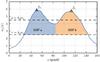 |
Fig. 1 Schematic illustration of the method used for SSP localization, applied to a one-dimensional case. The local maxima (triangle marker) are located using the maximum filter and the SSP are associated with each of the local maxima by applying the watershed flooding algorithm. In this example the SSP “a” associated with the position fa is defined by a region between 25 pix and 82 pix. |
3.2.1. Identification of significant structural patterns
An SSP is defined as a 2D region of enhanced intensity extracted at a given wavelet scale. To determine the extent and shape of individual SSP associated with significant local maxima, image segmentation needs to be performed. The segmentation relates each local maximum to a range of surrounding pixels that can be considered part of this local intensity enhancement. The map of significant coefficients mj is used for that purpose. The borders between individual regions are determined from the common minima located between the adjacent regions. This is achieved by watershed flooding (Beucher & Meyer 1993)1. Figure 1 illustrates the application of the watershed segmentation in a one-dimensional case.
The watershed segmentation is performed on −mj at all scales j with Fj as “water sources”, or markers. Each local maximum fa of Fj gives a region sj,a defined as ![\begin{equation} s_{j, a}(x, y) = \begin{cases} m_{j}(x, y) & \parbox[t]{.25\textwidth}\,\,\,{\rm if}\,\,\, (x, y)\,\,\, \text{is inside the watershed line of}\,\, f_a\\ 0 & \parbox[t]{.25\textwidth}{ otherwise. } \end{cases} \end{equation}](/articles/aa/full_html/2015/02/aa24566-14/aa24566-14-eq37.png) (5)The resulting SSP representation of an image at the scale j is finally derived as the group of regions:
(5)The resulting SSP representation of an image at the scale j is finally derived as the group of regions:  (6)An example of applying the SSP identification is shown in Fig. 4 for a simulated image of a compact radio jet.
4. Multiscale cross-correlation
To detect structural differences between two images of an astronomical object made at epochs t1 and t2, one needs to find an optimal set of displacements of the original SSP (described by the groups of SSP Sj,1,j = 1,...,J) that would match the SSP in the second image (described by Sj,2, j = 1,...,J). Cross-correlating Sj,1 and Sj,2 is a natural tool for this purpose. There are two specific issues that need to be addressed, however, to ensure that the cross-correlation analysis is reliable. First, a viable rule needs to be introduced to identify the relevant image area across which the cross-correlation is to be applied. The typical choices of using the full image area or manually selecting the relevant fraction of the image (cf. Pushkarev et al. 2012; Fromm et al. 2013) are not satisfactory for this purpose. Second, the probability of false matching needs to be minimized for features with sizes smaller than the typical displacement between the two epochs.
These two requirements can be met by multiscale cross-correlation (MCC), which combines the structural and positional information contained in Sj at all scales of the wavelet decomposition. The MCC uses a coarse-to-fine hierarchical strategy that is well known in image registration. This principle has first been used in Vanderbrug & Rosenfeld (1977) and Witkin et al. (1987), who used Gaussian pyramids. It was then extended to the wavelet transform by Djamdji et al. (1993) and Zheng & Chellappa (1993). We refer to Zitová & Flusser (2003) and Paulson et al. (2010) for a review on the different techniques developed in this area. However, none of theses algorithms can be directly applied for our purpose. The main reasons for this difficulty are the following:
-
1.
The images we consider are sparsely sampled (with structural displacements on the order of the PSF size or even larger) and do not offer a set of “ground-control points” that facilitate image registration (while this aspect is a critical feature of virtually all of the remote-sensing and computer-vision algorithms).
-
2.
The images are often dominated by optically thin structures (with the possibility of two or more independent structural features projected onto each other and often having different displacement or velocity vectors).
-
3.
The structural patterns do not have a defined or even preferred shape, and their shape may also vary from one image to another.
Considering that SWD SSP at the wavelet scale j have a typical size of 2j, the largest displacement detectable on the scale j must be smaller than 2j. Identification of the structural displacements can then begin from choosing J, the largest scale of the wavelet decomposition, such that it exceeds the largest expected displacement, but still satisfies the upper limit on J given by the largest scale containing statistically significant wavelet coefficients. After correlating SJ,1 with SJ,2, the respective correlations between Sj,1 and Sj,2 on smaller scales are restricted to within the areas covered by SJ,1 and SJ,2 in the two images. Alternatively, this approach can also be used iteratively, restricting correlations on a given scale j to within the areas of the correlated features identified at the j + 1 scale. This algorithm is illustrated in Fig. 2. Details of the procedure for relating SSP identified at different scales are discussed in the next section.
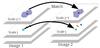 |
Fig. 2 Illustration of the feature-matching method using a coarse-to-fine strategy. The calculated displacement at a higher (larger) scale is used to constrain the determination of the feature displacements at a lower (smaller) scale. In this particular example, the displacement of the SSP at scale j + 1 is used as initial guess for displacements of its child SSPs at scale j. The initial guesses are subsequently refined by cross correlation. |
4.1. Multiscale relations
Multiscale relations between SSP identified at different spatial scales can be derived from the basic region properties. We note again that the sizes of SSP identified at the scale j are on the order of 2j. Hence, any two individual SSP sa and sb of Sj, identified around respective local maxima fa and fb, are separated from each other by at least 2j. This corresponds to the inequality 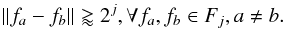 (7)If one determines a displacement Δj + 1,b of the SSP sj + 1,b at the scale j + 1 between two epochs t1 and t2, the following relation can be applied for the features of Fj that are inside sj + 1,b:
 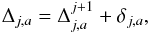 (8)for all fa ∈ Fj and fb ∈ Fj + 1, so that sj + 1,b(fa) > 0 and the condition
  is satisfied. From Eqs. (7)and (8), it also follows that
 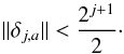 (9)Based on these relations, we adopted the following MCC algorithm to detect structural changes between two images of an astronomical object:
-
1.
The largest scale J of a wavelet decomposition is chosen such that either the largest expected displacement is smaller than 2J or J corresponds to the largest scale with statistically significant wavelet coefficients.
-
2.
Displacements of SSP features are determined at the largest scale J. For this calculation, all
 are set to zero, and ΔJ,a = δJ,a is calculated for each SSP.
 -
3.
At each subsequent scale j (j<J),
 is determined first by adopting the displacement ΔJ,a measured at the j + 1 scale for the SSP in which the given j-scale region sj,a falls. Then the total displacement for this SSP is given by
  .
.
In this algorithm, the only quantity that needs to be calculated at each scale is the relative displacement δj,a. This quantity is bound by Eq. (9)and, within this bound, it can be determined reliably from the cross-correlation.
4.2. Correlation criteria for MCC
The correlation is calculated between a reference image r and a target image t, with the time order of the two images not playing any role. The correlation coefficients can be estimated using a number of different correlation criteria (see Giachetti 2000, for a review). The most commonly used criteria are the cross correlation, 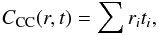 (10)and the sum of squared differences,
 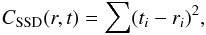 (11)with i the pixel index. The tolerance to an offset between the reference and the target image is obtained by subtracting the mean value of the image intensity (zero-mean correlation). Similarly, tolerance to scale change is obtained by dividing the root-mean-square of the image intensity (normalized correlation).
The MCC algorithm is required to be insensible to both the image offset and scale change. The zero-mean normalized cross correlation (ZNCC) and zero-mean normalized sum of the squared difference (ZNSSD) can be applied for this purpose. Pan et al. (2010) have demonstrated that these two criteria are equivalent. MCC uses the ZNCC method, based on its excellent computational performance (Lewis 1995). The ZNCC is given by 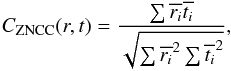 (12)with
  , and
, and  being the mean of r. This criterion reaches its highest unity value when the reference and target image are identical.
To detect structural changes between the reference and target images, each single SSP sj,a of the reference image is cross correlated with the target image. As every SSP is constrained to be located within a specific region, one is actually only interested in determining the correlation over that region. To achieve this, a weighting function, ω is introduced, which is normalized to unity and provides ω ≡ 0 everywhere except inside the region containing the SSP of interest. A weighted zero-mean normalized cross correlation (WZNCC) can then be defined as 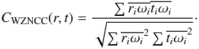 (13)
(13)
4.3. Detection of SSP displacements
As shown in Sect. 4.1, the displacements of individual features are determined starting from the largest scale and progressing to the finest scale of the wavelet decomposition. For each SSP at the scale j, an initial guess for its displacement is provided by the displacement measured for the region at the scale j + 1, which includes the SSP in question. The initial guess is then refined via the cross correlation.
This simple procedure is complicated by the fact that individual SSP may merge, split, or overlap as a result of structural changes occurring between the two observations. This means that the displacement for which the cross correlation is maximized does not necessarily provide the correct solution. Such a situation in exemplified in Fig. 3. In this example, SSP b is moving faster than SSP a. As a consequence, cross correlating the SSP b at the epoch t1 with wj,t2 yields the global maximum at  and a local maximum at
  . The formal cross-correlation solution will be incorrect in this case. To avoid such errors (or at least to reduce their probability), it is necessary to cross-identify groups of close SSP that can be related (i.e., causally connected) to each other in the two images. The cross correlation can then be applied to these groups as well as to their individual members, so that a set of possible solutions is found for all SSP, and the final solution is determined through a minimization analysis applied to the entire group of SSP.
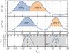 |
Fig. 3 Schematic illustration of the detection method used for displacement measurements in a one-dimensional case. In the upper two panels the wavelet decomposition at a scale j of the reference (top panel) and target image is plotted, with two detected SSP marked with colors and letters. The x-axis of each panel is given in pixels. The result of WZNCC between SSP b and the target image is plotted below in the third panel. Two potential displacements are identified within the bounds (gray area) defined by Eq. (9)and the initial displacement guess |

At the first step of this procedure, subsets of features Gj are defined that are considered to be interrelated. As was discussed in Sect. 4, at the scale j, fa is independent from fb if ∥ fa − fb ∥ > 2j + 1. Then,  (14)with
  (15)At the second step, cross correlation is applied, yielding several possible displacement vectors for each feature of such a group. Considering the multiscale relations described in Sect. 4.1, the correlation coefficients at δ = (δx,δy) can be calculated for a given feature fa of a group Gj,u:
 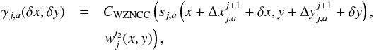 (16)with ∥ δ ∥ < 2j.
As illustrated by the example shown in Fig. 3, for complex and strongly evolving structures, it is possible that formally the best cross-correlation solution provided by the largest γj,a,max may be spurious. Hence, to avoid such spurious estimates of the displacement vectors, all local maxima of γj,a that are above a certain threshold κ (with κ usually set ≥0.8) may be considered as possibly relevant solutions. These local maxima are found using the maximum filter method described in Sect. 3.2.
After identifying all relevant local maxima, the WZNCC of the group of features is calculated for each possible group solution, and we select the combination of individual displacement δ that maximizes the group correlation. This operation is repeated for all groups of features Gj,u. This approach provides a robust estimate of the statistically significant structural displacement vectors across the entire image and at each structural scale.
In summary, our cross-correlation procedure comprised the following main steps:
-
1.
Individual initial displacements and bounds are determined for each SSP using the relations of Eqs. (8)and (9).
-
2.
Groups of causally connected features are defined.
-
3.
Cross-correlation analysis is performed using the WZNCC for the groups and each of their elements, resulting in a set of potential displacements.
-
4.
The final SSP displacements are determined by selecting a combination of individual displacements that maximizes the overall group correlation.
4.4. Overlapping multiple displacement vectors
In images of optically thin structures, several physically disconnected regions with different sizes and velocities may overlap, causing additional difficulties for a reliable determination of structural displacements (observations of transversely stratified jets would be one particular example of such a situation). Using the partial independence of SWD SSP recovered at different wavelet scales, the MCC method can partially recover these overlapping displacement components. The largest detectable displacement inside a region is determined by the largest wavelet scale j for which this region can be described by at least two SSP. Then, as described in Sect. 4.1, the largest detectable displacement would be 2j. If velocity gradients or multiple velocity components are expected inside this region, then this might not be sufficient and the analysis might have to be started again at a wavelet scale that describes the desired region by three or four different SSP.
The multiscale relations described in Sect. 4.1 rely on the assumption that SSP detected at a scale j move, on average, like their parent SSP detected at scale j + 1. This assumption sets limits for detecting different speeds at different scales. Between two scales j + 1 and j, this limit, determined by Eq. (8), is on the order of 2j. As the velocity difference approaches this limit, matching becomes more difficult. If a very strong stratification or distinctly different overlapping velocity components are expected, it is possible to relax this constraint by introducing a tolerance factor ktol in Eq. (9),  (17)This modification may increase the formal probability of spurious matches, but the overall negative effect of introducing the tolerance factor will be largely moderated by the cross-correlation part of the algorithm. A similar limit applies if the gradient of velocity inside an SSP is on the order of the SSP size.
5. Testing the WISE algorithm
To test the application of the WISE algorithm, simulated images of optically thin relativistic jets were prepared that contained divergent and overlapping velocity vectors manifested by structural displacements generated for a range of spatial scales.
The simulated jet had an overall quasi-conical morphology, with a bright and compact narrow end (“base” of the jet) and smooth underlying flow pervaded by regions of enhanced brightness (often called “jet components”) moving with velocities that varied in magnitude and direction. The underlying flow was simulated by a Gaussian cylinder with FWHM wjet evolving with the following relation: 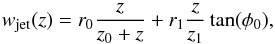 (18)where r0 is the width at the base of the jet, z0 the axial z-coordinate of the jet base, and z1 the z-coordinate of the point after which w(z) increase linearly with an opening angle of φ0, and intensity ijet evolving with the relation:
 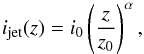 (19)where α is the damping factor.
The jet base was modeled by a Gaussian component located on the jet axis, at the position z0. The moving features, also modeled by Gaussian components (with randomly distributed parameters), were added in the area defined by the jet after z1. The resulting image was finally convolved with a circular or elliptical beam to study the effect of different instrumental PSFs on the WISE reconstruction of the simulated structural displacements. An example of a simulated image together with the SSP detected with the SWD at three different scales is shown in Fig. 4.
To evaluate the performance of WISE, two sets of tests were performed. The first set consisted of testing the SWD algorithm for sensitivity to features at low SNR (sensitivity test) and for distinguishing close and overlapping patterns (separation test). At the second stage of testing, the full WISE algorithm (combining the SWD and the MCC parts) was applied to evaluate the sensitivity of the method of detecting spatial displacements of individual patterns (displacement test). In the following discussion, we define the SNR of a feature as its peak intensity over the noise level in the image.
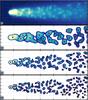 |
Fig. 4 Top panel: shows a map of a simulated radio jet as described in Sect. 5. Lower panels: show the resulting SWD decomposition obtained at scales of 1.6, 0.8, and 0.4 beam size. |
5.1. Sensitivity test
This test was designed to represent as closely as possible the generic use of the SWD algorithm for detecting and classifying structural patterns in astronomical images. The test was performed on a simulated image of a jet, as illustrated in Sect. 5. For this particular simulation a circular PSF with a FWHM of 10 pixels was applied. The morphology of the underlying jet was given by the initial width r0 = 5 FWHM and an opening angle of 8°.
Superimposed on the smooth underlying jet background, Gaussian features with different sizes and intensities were then added. The features were separated widely enough from each other to avoid overlapping. The SWD method was applied to the simulated image, and the SWD detections were then compared to the positions, sizes, and intensities of the simulated features. For the purpose of comparison, we also performed a simple direct detection (DD), which consist of detecting local maxima that are above a certain threshold directly on the image. Similarly as for the SWD detection, the threshold for the DD method was set to kdσn, where kd is the detection coefficient as defined in Sect. 3.2, and σn the standard deviation of the noise in the image. When we determined whether a detected feature corresponded to a simulated one, we used a tolerance of 0.2 FWHM of the beam size on the position.
Table 1 compares the performance of the two methods. The SWD method successfully recovered 95% of the extended features at SNR ≳ 6 with a low false-detection rate (FDR) for kd ≥ 4. This makes it a reliable tool for detecting the statistically significant structures in astronomical images. In this particular test the SWD method outperform the DD method by a factor of ≈4.
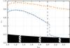 |
Fig. 5 Characterization of the separability, rs, of two close features with varying FWHM ratio, κw. Separation limit is determined for the SWD method (blue cross) and a direct detection method (yellow cross) as introduced in Sect. 5.1. The gray hatched area is the region in the plot for which the separation between the two features is lower than 2 pixels. |
Performance of the WDS detection compared to a direct detection (DD) in terms of SNR at which at 95% of the simulated features are detected.
5.2. Separation tests
The separation tests were designed to characterize the ability of the SWD method to distinguish two close features. In this test, the images structure comprised two Gaussian components of finite size that were partially overlapping. The two components were defined by their respective SNR, S1 and S2 and FWHM, w1 and w2, and they were separated by a distance Δs. For the purpose of quantifying the test results, the fractional component separation rs = 2Δs/ (w1 + w2) was introduced. The tests determined the smallest rs for various combinations of the component parameters at which the two features are detected. The performance of the SWD algorithm was again compared with results from applying the DD method introduced in Sect. 5.1.
In the first separation test, the ratio κw = w1/w2 was varied while setting S1 = S2 = 20. Note that the features partially overlapped at their half-maximum level for rs ≤ κw/ (1 + κw). The results of this test are shown in Fig. 5, with SWD always performing better than the DD. In addition to this, the evolution of smallest detectable rs with κw indicates two different regimes for SWD. For 1 ≤ κw< 2, SWD progressively outperforms DD, with the difference between the two increasing as κw increases. At κw ≥ 2, SWD undergoes a fundamental transition, with both features ultimately being always detected (at the 2-pixel separation limit). This is the result of the multiscale capability of the SWD to identify and separate power concentrated on physically different scales.
In the second separation test, the ratio ϵs = S1/S2 was varied for features with w1 = w2 = 10 pixels. The result demonstrates that SWD performs better than DD, with improvement factors rising from 30% to 50% with increasing SNR ratio ϵs.
Both tests show that SWD is successful at resolving out two close and partially overlapping features. Assuming that the simulated component width w2 in both tests is similar to the instrumental PSF, rs can be interpreted as ≈2 / (1 + κw) PSF, implying that SWD successfully distinguishes two marginally resolved features separated by ≈ , which is close to the expected limit
 ![\begin{eqnarray*} r_\mathrm{s,lim} \approx \frac{2}{\sqrt{\pi}} \ln\left[\frac{S_2(1+\epsilon_\mathrm{s})+1} {S_2(1+\epsilon_\mathrm{s})}\right]^{1/2} \frac{(1+\epsilon_\mathrm{s})^2}{\sqrt{1+\epsilon_\mathrm{s}^2}}\,\times\, \mathrm{PSF} \end{eqnarray*}](/articles/aa/full_html/2015/02/aa24566-14/aa24566-14-eq149.png) for resolving two close features (cf. Bertero et al. 1997).
for resolving two close features (cf. Bertero et al. 1997).
5.3. Structural displacement test
These tests used the full WISE processing on a set of two simulated jet images, first using the SWD algorithm to identify SSP features in each of the images, then applying the MCC algorithm to cross-correlate the individual SSP and to track their displacements from one image to the other. The jet images were simulated using the procedure described in the beginning of this section. A total of 500 elliptical features were inserted randomly inside the underlying smooth jet, with their SNR spread uniformly from 2 to 20 and the FWHM of the features ranging uniformly from 0.2 to 1 beam size. The simulated structures were convolved with a circular Gaussian (acting as an instrumental PSF) with a FWHM of 10 pixels. A damping factor α of −0.3 was used.
Positional displacements were introduced to the simulated features in the second image. The simulated displacements have both regular and stochastic (noise) components introduced as follows:  (20)where fx and fy are the regular components of the displacement, and Gx and Gy are two random variables following the Gaussian distributions described by the respective means ⟨ Gx ⟩, ⟨ Gy ⟩ and standard deviations σx, σy. After the two images were generated, SSP were detected independently in each of them with the SWD and were subsequently cross-identified with the MCC.
5.3.1. Accelerating outflow
This displacement test explores a kinematic scenario describing an accelerating axial outflow with a sinusoidal velocity component transverse to the main flow direction: 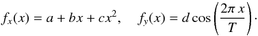 (21)Results of the WISE application are shown in Figs. 6, 7 for a = −2, b = 0.02, c = 0.00012, d = 10, T = 200, for the stochastic displacement components with σx = σy = 2 and σx = σy = 5 (0.2 FWHM and 0.5 FWHM), respectively (all linear quantities are expressed in pixels). The largest expected displacement between the two images is 40 pixels. The WISE analysis was performed on scales 2–6 (corresponding to 4–64 pixels).
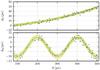 |
Fig. 6 WISE decomposition and analysis of a simulated jet with an accelerating sinusoidal velocity field. The input velocity field (green line) is defined analytically and modified with a Gaussian stochastic component with an rms of 0.28 FWHM of the convolving beam. The rms margins due to the stochastic component are represented by the yellow-shaded area. A total of 87% of all detected SSP have been successfully matched by WISE. The detected positional changes (blue crosses) show rms deviations of 0.19 and 0.20 FWHM (in x and y coordinates, respectively) from the simulated sinusoidal field. |
The comparison between the simulated displacements and the displacements detected by WISE reveals an excellent performance of the matching algorithm. To assess this performance, we computed the root mean square of the discrepancies between the simulated and detected displacements: 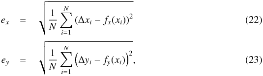 where Δxi, Δyi are the measured x and y components of the displacement identified for the ith simulated component, and xi is the position of that component along the x axis in the first simulated image. The ex and ey determined from the WISE decomposition do not exceed the σx and σy of the simulated data. For the first we obtain ex = 0.19 and ey = 0.20, while for the second test, we obtain ex = 0.43 and ey = 0.42. The number of positively matched features decreases with increasing stochastic component of the displacements, but the errors of WISE decomposition always remain within the bounds determined by the simulated noise.
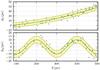 |
Fig. 7 Same as in Fig. 6, but for the simulated stochastic component with an rms of 0.71 FWHM of the convolving beam. The total of 54% of all identified SSP have been successfully matched between the two simulated images. The respective rms of the deviations of the detected displacements from the analytic sinusoidal velocity field are 0.43 FWHM and 0.42 FWHM, in x and y coordinates, respectively. |
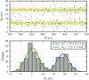 |
Fig. 8 WISE decomposition and analysis of a simulated jet with two speed components. Two groups of features evolving at two different speeds are simulated. Upper panel: blue crosses show the displacements detected by WISE from successive pairs in four simulated images (epochs). Green lines and orange shades indicate the two simulated displacements and rms of the Gaussian stochastic component. Lower panel: the histogram of the detected positional changes reveals two distinct components of the speed. The mean values of the speed and their rms, indicated in the top right corner, agree well with the simulated displacements Δx1 = 5 px and Δx2 = 20 px. |
These comparisons indicate that WISE performs very well even in the case of relatively large spurious and random structural changes (which may result from deconvolution errors, phase noise, and incompleteness of the Fourier domain coverage by the data). Because such spurious displacement is expected at a level of ≲FWHM/ , WISE should be able to reliably identify displacement in regions detected at SNR ≳ 4.
5.3.2. Two-fluid outflow
The purpose of this test was to investigate the possibility of using WISE to detect multiple velocity components in optically thin materials in which structures moving at different speeds overlap. To simulate such a two-fluid outflow, the initial set of features was divided into two groups F1 and F2. The SNR and FWHM of these features were derived from the same distribution. The simulated displacements, Δ1,2, were oriented longitudinally (along the x-axis) in the outflow and were the same in all of the features of a given group, with Δx1 = a and Δx2 = b, for the feature in F1 and F2, respectively.
Results of the WISE application are shown in Fig. 8 for a = 5 px, b = 20 px and σx = σy = 2 px (with a PSF size of 10 px). It is expected that a combination of more than two epochs is required to obtain enough positional changes to distinguish the two different values of the speed. In this case, combining the total of four epochs is found to be necessary. The speeds of individual features were determined through a statistical analysis of the detected displacements. The distribution of the detected displacements shown in Fig. 8 is bimodal, with two clearly separated peaks, and it can be used to derive the mean speed and its rms for each of the two simulated flow components. This yields Δx1 = 19.2 ± 2.7 px and Δx2 = 5.2 ± 3.0 px, which agrees well with the displacements used to simulate the two components of the flow.
6. Applications to astronomical images
We have tested the performance of WISE on astronomical images by applying it to several image sequences obtained as part of the MOJAVE long-term monitoring program of extragalactic jets with very long baseline interferometry (VLBI) observations (Lister et al. 2013, and references therein). The particular focus of the tests is on two prominent radio jets in the quasar 3C 273 and the Seyfert galaxy 3C 120. These jets show a rich structure, with a number of enhanced brightness regions inside a smooth and slowly expanding flow. This richness of structure on the one hand has always been difficult to analyze by means of fitting it by two dimensional Gaussian features, on the other hand, it has always suggested that the transversely resolved flows may manifest a complex velocity field, with velocity gradients along and across the main flow direction (cf. Lobanov & Zensus 2001; Hardee et al. 2005).
The MOJAVE observations, with their typical resolution of 0.5 milliarcsecond (mas), transversely resolve the jets in both objects and, in addition, they also reveal apparent proper motions of 3 mas/year in 3C 120 (Lister et al. 2013), which makes these two jets excellent targets for attempting to determine the longitudinal and transverse velocity distribution.
The WISE analysis was applied to the self-calibrated hybrid images provided at the data archive of the MOJAVE survey2. The results of WISE algorithm were compared to the MOJAVE kinematic modeling of the jets based on the Gaussian model fitting of the source structure (see Lister et al. 2013, for a detailed description of the kinematic modeling).
6.1. Analysis of the images
For each object, the MOJAVE VLBI images were first segmented using the SWD algorithm, with each image analyzed independently. The image noise was estimated by computing σj at each wavelet scale, as described in Sect. 3.1. Based on these estimates, a 3σj thresholding was subsequently applied at each scale. This procedure provides a better account for the scale dependence of the noise in VLBI images (Lal et al. 2010; Lobanov 2012), which is expected to result from a number of factors including the coverage of the Fourier domain and deconvolution.
Following the segmentation of individual images, MCC was performed on each consecutive pair of images, providing the displacement vectors for all SSP that were successfully cross-matched. The images were aligned at the position of the SSP that was considered to be the jet “core” (which is typically, but not always, the brightest region in the jet). This was done to account for possible positional shifts resulting from self-calibration of interferometric phases and for potential positional shifts (core shift) due the opacity at the observed location of the jet base (Lobanov 1998b; Kovalev et al. 2008).
For SSP that were cross-identified over a number of observing epochs, the combination of these displacements provided a two-dimensional track inside the jet. The track information from several scales was also combined whenever a given SSP was cross-identified over several spatial scales.
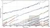 |
Fig. 9 Core separation plot of the most prominent features in the jet of 3C 273. The model-fit based MOJAVE results (dashed lines) are compared with the WISE results (solid lines) obtained for SWD scales 3 and 4 (selected to match the effective resolution of WISE to that of the Gaussian model fitting employed in the MOJAVE analysis). A detailed analysis, also including SWD scales 1 and 2, was performed for the observations made between 11/2003 and 12/2006 (gray box); the results are shown in Fig. 11. |
6.1.1. Jet kinematics in 3C 273
The MOJAVE database contains 69 images of 3C 273, with the observations covering the time range from 1996 to 2010 and providing, on average, one observation every three months. The SWD was performed with four scales, ranging from 0.2 mas (scale 1) to 1.6 mas (scale 4).
For the MCC part of WISE, the individual images were aligned at the positions of their respective strongest and most compact components (“core” components) as identified by the MOJAVE model fits. The kinematic evolution of most of the detected SSP is fully represented by the MCC results obtained for a single selected SWD scale. However, long-lived features in the flow could eventually expand so much that the wavelet power associated with a specific SSP would be shifted to a larger scale, and the full evolution of such a feature was described by a combination of MCC applications to two or more SWD scales.
The core separations of individual SSP obtained from WISE decomposition are compared in Fig. 9) with the results from the MOJAVE kinematic analysis based on the Gaussian model fitting of the jet structure. To provide this comparison, the effective resolution of WISE must be reduced by excluding the scales 1–2 from the consideration. Comparison of the MOJAVE and WISE results in Fig. 9 indicates that WISE detects consistently nearly all the components identified by the MOJAVE model fitting analysis, with a very good agreement on their positional locations and separation speeds.
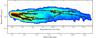 |
Fig. 10 Two-dimensional tracks of the SSP detected by WISE at scales 3–4 of the SWD and compared in Fig. 11 with the features identified in the MOJAVE analysis of the images. The tracks are overplotted on a stacked-epoch image of the jet rotated by an angle of 0.55 radian. Colors distinguish individual SSP continuously tracked over certain period of time. Several generic “flow lines” are clearly visible in the jet. These patterns are difficult to detect with the standard Gaussian model fitting analysis. The image is rotated. |
The two-dimensional tracks of the WISE features detected with this procedure are shown in Fig. 10, overplotted on a single-epoch image of the jet. The displacement tracks clearly show several “flow lines” threading the jet, which can be associated with the instability pattern identified in it (Lobanov & Zensus 2001). Some of these tracks can also be identified in Gaussian model fitting, but only if there is no substantial structural variations across the jet. If this is not the case, Gaussian model fitting becomes too expensive and too unreliable for the purpose of representing the structure of a flow. In this situation, WISE provides a better way to treat the structural complexity. We therefore conclude that WISE can be applied for the task of automated structural analysis of VLBI images of jets (and similar sequences of images of objects with evolving structure), yielding a great increase in the speed of the analysis (analyzing 69 images of 3C 273 took about ten minutes of computing, while the model fitting of these images required several days of the researchers’ time).
However, WISE can certainly go beyond the resolution of Gaussian model fitting by also including scales that are smaller than the transverse dimension of the flow. An example of such an improvement is shown in Fig. 11, which focuses on MOJAVE observations of 3C 273 made between November 2003 and December 2006. At core separations larger than about 2 mas, WISE persistently detects several features at locations where the Gaussian model fits have been restricted to representing the structure with a single component. This is a clear sign of transverse structure in the flow, which is illustrated well by the respective displacement tracks shown in Fig. 12. These tracks provide strong evidence for a remarkable transverse structure of the flow, with three distinct flow lines clearly present inside the jet. These flow lines evolve in a regular fashion, suggesting a pattern that may rise as a result of Kelvin-Helmholtz instability, possibly due to one of the body modes that have been previously identified in the jet based on a morphological analysis of the transverse structure (Lobanov & Zensus 2001). That analysis also implied that the flow pattern probably rotates counterclockwise, and this rotation is consistent with the general southward bending of the displacement vectors (particularly visible in Fig. 12 at distances of 4.5–6 mas).
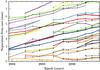 |
Fig. 11 Core separation plot of features detected in a detailed analysis of the jet of 3C 273, which includes the SWD scales 1 and 2. Dashed lines show the MOJAVE model fit components, colored tracks present the SSP detected and tracked by WISE. At core separations ≳2 mas, WISE detects more significant features as the jet becomes progressively more resolved in the transverse direction (which also indicates that the structural description of the jet provided by Gaussian model fitting is no longer optimal). |
6.1.2. 3C 120
The MOJAVE database for 3C 120 comprises 87 images from observations made in 1996–2010, averaging to one observation every three months (but with individual gaps as long as one year). We prepared these images for WISE analysis using the same approach as applied for 3C 273. To ensure sensitivity to the expected displacements of ≲3 mas between subsequent images, we applied SWD on five scales, from 0.2 mas (scale 1) to 3.2 mas (scale 5).
Applied to the MOJAVE images of 3C 120, WISE detects a total of 30 moving SSP. The evolution of 24 SSP is fully traced at the SWD scale 2 (0.4 FWHM), and combining two SWD scales is required to describe the evolution of the six remaining SSP. The resulting core separations of the SSP plotted in Fig. 13 generally agree very well with the separations of the jet components identified in the MOJAVE Gaussian model fit analysis. For the moving features, displacements as large as ~3 mas were reliably identified during the periods with the least frequent observations.
The only obvious discrepancy between the two methods are the quasi-stationary features that are identified in the MOJAVE analysis, but are absent from the WISE results. A closer inspection of the wavelet coefficients recovered at the SWD scale 1 does not yield a statistically significant detection of an SSP at the location of the MOJAVE stationary component either.
The stationary feature identified in the MOJAVE analysis is often separated by less than 1 FWHM from the bright core, while it is substantially (factors of ~50–100) weaker than the core. This extreme flux density ratio between two clearly overlapping components may impede identifying the weaker feature against the formal thresholding criteria of WISE. The fact that the Gaussian model fitting was performed in the Fourier domain (not affected by convolution) may have given it an advantage in this particular setting. Subjective decision making during the model fitting may also have played a role in the resulting structural decomposition.
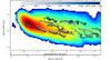 |
Fig. 12 Two-dimensional tracks of SSP detected in 3C 273 at the scale 2 of SWD for the epochs between 11/2003 and 12/2006. The tracks correspond to the features plotted in Fig. 11. The colors of the displacement vectors indicate the measurement epoch as shown in the wedge at the top of the plot. The plot confirms the significant transverse structure in the jet, with up to three distinct flow lines showing strong and correlated evolution. The apparent inward motion detected in a nuclear region (0–0.3 mas) is most likely an artifact of a flare in the jet core. |
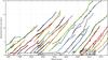 |
Fig. 13 Core-separation plot of the features identified in the jet of 3C 120. The model-fit based MOJAVE results (dashed lines) are compared with the WISE results (solid lines) obtained for SWD scales 2 and 3 (selected to match the effective resolution of WISE to that of the Gaussian model fitting employed in the MOJAVE analysis). |
Reaching a firm conclusion on this matter would require assessing the statistical significance of the model fit components identified with the stationary features and performing the SWD separation test for extreme SNR ratios. We defer this to future analysis of the data on 3C 120, while noting again that WISE has achieved its basic goal of providing an effective automated measure of kinematics in a jet with remarkably rapid structural changes.
The magnitude of the structural variability of the jet in 3C 120 is further emphasized in Fig. 14, which shows the two-dimensional tracks of the SSP identified with WISE. The shape of individual tracks suggests a helical morphology, consistent with the patterns predicted from modeling the jet in 3C 120 with linearly growing Kelvin-Helmholtz instability (Hardee et al. 2005). In this framework, the observed evolution of the component tracks is consistent with the pattern motion of the helical surface mode of the instability identified by Hardee et al. (2005) to have a wavelength of ~3.1 jet radii and propagating at an apparent speed of ~0.8 c.
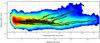 |
Fig. 14 Two-dimensional tracks of SSP detected in 3C 120 at scale 2 of SWD. The colored tracks correspond to the features plotted in Fig. 13 in the same color. The tracks are overplotted on a stacked-epoch image of the jet rotated by an angle of 0.4 radian. The plot confirms the significant and evolving transverse structure in the jet, with individual tracks underlying the long-term evolution of the flow, which becomes particularly prominent at core separations of ≳6 mas. |
Hardee et al. (2005) also suggested that the structure of the flow is strongly dominated by the helical surface mode, which may explain the apparent lack of structural detail uncovered by WISE on the finest wavelet scale. In this case, observations at a higher dynamic range would be needed to reveal higher (and weaker) modes of the instability developing in the jet on these spatial scales. Altogether, the example of 3C 120 again demonstrates the reliability of the WISE decomposition and analysis of a structural evolution that can be inferred from comparing multiple images of an astronomical object.
7. Conclusions
The WISE method we presented here offers an effective and objective way to classify structural patterns in images of astronomical objects and track their evolution traced by multiple observations of the same object. The method combines automatic segmented wavelet decomposition with a multiscale cross-correlation algorithm, which enables reliable identification and tracking of statistically significant structural patterns.
Tests of WISE performed on simulated images demonstrated its capabilities for a robust decomposition and tracking of two-dimensional structures in astronomical images. Applications of WISE on the VLBI images of two prominent extragalactic jets showed the robustness and fidelity of results obtained from WISE compared with those coming from the “standard” procedure of using multiple Gaussian components to represent the observed structure. The inherent multiscale nature of WISE allows it also to go beyond the effective resolution of the Gaussian representation and to probe the two-dimensional distribution of structural displacements (hence probing the two-dimensional kinematic properties of the target object).
In addition to this, the multiscale approach of WISE has several other specific advantages. First, it allows simultaneous detection of unresolved and marginally resolved features as well as extended structural patterns at low SNR. Second, the method provides a dynamic and structural scale-dependent account of the image noise and uses it as an effective thresholding condition for assessing the statistical significance of individual structural patterns. Third, multiple velocity components can also be distinguished by the method if these components act on different spatial scales – this can be a very important feature to study the dynamics of optically thin emitting regions such as stratified relativistic flows, with a combination of pattern and flow speed and strong transverse velocity gradients.
Combining several scales also improved the cross-correlation employed by WISE, ensuring a reliable performance of the method in the case of severely undersampled data (with the structural displacement between successive epochs becoming larger than the dimensions of the instrumental point spread function).
In its present realization, WISE performs well on structures with moderate extent, while it may face difficulties in correctly identifying continuous structural details in which one of the dimensions is substantially smaller than the other (e.g., filamentary structure and thread-like features). If the ratio between the largest and smallest dimensions of this structure is lower than the ratio of the largest and smallest scales of WISE decomposition, the continuity of this structure may in principle be recognized. For more extreme cases, WISE will break the structure into two or more SSP that are considered independent. A remedy for this deficiency may be found in considering groups of SSP during the MCC part of WISE, or by applying more generic approaches to feature identification (e.g., shapelets; cf. Starck & Murtagh 2006).
Another probable, requiring additional attention is the scale crossing of individual features that may occur as a result of expansion (as was illustrated by the example of 3C 273) or the particular evolution of a complex three- dimensional emitting region projected onto the two-dimensional picture plane. At the moment, this problem has to be treated manually and outside of WISE, but an automated approach is clearly desired. One possibility here is to use the wavelet amplitudes associated with the same SSP at different scales and to select the dominant scale adaptively based on the comparison of these amplitudes and their changes from one observing epoch to another.
Implementing this step may also require implementing a reliable error estimation for the locations, flux densities, and dimensions of SSP identified by WISE. This can be done on the basis of SNR estimates performed at each individual scale of WISE decomposition. Generically, it is expected that and SSP detected with a given SNR at a particular wavelet scale lw would have its positional and flux errors ∝lw/SNR-1, while the error on the SSP dimension would be ∝lw/SNR− 1 / 2 (cf. Fomalont 1999). Such estimates can be implemented as a zeroth-order approach, but a more detailed investigation of the error estimates for the segmented wavelet decomposition is clearly needed.
The watershed flooding earns its name from effectively corresponding to placing a “water source” in each local minimum and “flooding” the image relief from each of these “sources” with the same speed. The moment that the floods filling two distinct catchment basins start to merge, a dam is erected to prevent mixing of the floods. The union of all dams constitutes the watershed line.
Acknowledgments
This research has made use of data from the MOJAVE database that is maintained by the MOJAVE team (Lister et al. 2009).
References
- Adams, N. J., & Williams, C. K. I. 2003, Image and Vision Computing, 21, 865 [CrossRef] [Google Scholar]
- Agarwal, S., Awan, A., & Roth, D. 2003, IEEE Transactions on Pattern Analysis and Machine Intelligence, 26, 1475 [Google Scholar]
- Ahuja, N., Lertrattanapanich, S., & Bose, N. 2005, Vision, Image and Signal Processing, IEE Proc., 152, 659 [Google Scholar]
- Arulampalam, M. S., Maskell, S., Gordon, N., & Clapp, T. 2002, IEEE Transactions on Signal Processing, 50, 174 [Google Scholar]
- Bach, U., Krichbaum, T. P., Middelberg, E., Alef, W., & Zensus, A. J. 2008, in The role of VLBI in the Golden Age for Radio Astronomy [Google Scholar]
- Belongie, S., Malik, J., & Puzicha, J. 2002, IEEE Transactions on Pattern Analysis and Machine Intelligence, 24, 509 [CrossRef] [Google Scholar]
- Bertero, M., Boccacci, P., & Piana, M. 1997, in Lect. Notes Phys. 486 (Berlin: Springer Verlag), eds. G. Chavent, & P. C. Sabatier, 1 [Google Scholar]
- Beucher, S., & Meyer, F. 1993, Opt. Eng., 34, 433 [Google Scholar]
- Biretta, J. A., Zhou, F., & Owen, F. N. 1995, ApJ, 447, 582 [NASA ADS] [CrossRef] [Google Scholar]
- Clark, B. G. 1980, A&A, 89, 377 [NASA ADS] [Google Scholar]
- Cornwell, T. J. 2008, IEEE Journal of Selected Topics in Signal Processing, 2, 793 [Google Scholar]
- Djamdji, J.-P., Bijaoui, A., & Maniere, R. 1993, Proc. SPIE, 1938, 412 [NASA ADS] [CrossRef] [Google Scholar]
- Doucet, A., & Gordon, N. J. 1999, in Signal and Data Processing of Small Targets, ed. O. E. Drummond, SPIE Conf. Ser., 3809, 241 [Google Scholar]
- Doucet, A., & Wang, X. 2005, IEEE Signal Processing Magazine, 22, 152 [NASA ADS] [CrossRef] [Google Scholar]
- Fomalont, E. B. 1999, in Synthesis Imaging in Radio Astronomy II, eds. G. B. Taylor, C. L. Carilli, & R. A. Perley, ASP Conf. Ser., 180,301 [Google Scholar]
- Fromm, C. M., Ros, E., Perucho, M., et al. 2013, A&A, 557, A105 [NASA ADS] [CrossRef] [EDP Sciences] [Google Scholar]
- Giachetti, A. 2000, Image and Vision Computing, 18, 247 [Google Scholar]
- Hardee, P. E., Walker, R. C., & Gómez, J. L. 2005, ApJ, 620, 646 [NASA ADS] [CrossRef] [Google Scholar]
- Högbom, J. A. 1974, A&AS, 15, 417 [NASA ADS] [Google Scholar]
- Holschneider, M., Kronland-Martinet, R., Morlet, J., & Tchamitchian, P. 1989, in Wavelets. Time-Frequency Methods and Phase Space, eds. J.-M. Combes, A. Grossmann, & P. Tchamitchian, 286 [Google Scholar]
- Hummel, C. A., Muxlow, T. W. B., Krichbaum, T. P., et al. 1992, A&A, 266, 93 [NASA ADS] [Google Scholar]
- Kovalev, Y. Y., Lobanov, A. P., & Pushkarev, A. B., & Zensus, J. A. 2008, A&A, 483, 759 [NASA ADS] [CrossRef] [EDP Sciences] [Google Scholar]
- Lal, D. V., Lobanov, A. P., & Jiménez-Monferrer, S. 2010 [arXiv:1001.1477] [Google Scholar]
- Lewis, J. 1995, Vision Interface, 10, 120 [Google Scholar]
- Lister, M. L., Aller, H. D., Aller, M. F., et al. 2009, AJ, 137, 3718 [NASA ADS] [CrossRef] [Google Scholar]
- Lister, M. L., Aller, M. F., Aller, H. D., et al. 2013, AJ, 146, 120 [NASA ADS] [CrossRef] [Google Scholar]
- Lobanov, A. P. 1998a, A&AS, 132, 261 [NASA ADS] [CrossRef] [EDP Sciences] [Google Scholar]
- Lobanov, A. P. 1998b, A&A, 330, 79 [NASA ADS] [Google Scholar]
- Lobanov, A. P. 2012, in Square Kilometre Array: Paving the Way for the New 21st Century Radio Astronomy Paradigm, eds. D. Barbosa, S. Anton, L. Gurvits, & D. Maia (Belrin Heidelrberg: Springer-Verlag), 75 [Google Scholar]
- Lobanov, A. P., & Zensus, J. A. 1999, ApJ, 521, 509 [NASA ADS] [CrossRef] [Google Scholar]
- Lobanov, A. P., & Zensus, J. A. 2001, Science, 294, 128 [Google Scholar]
- Lobanov, A., Hardee, P., & Eilek, J. 2003, New A Rev., 47, 629 [Google Scholar]
- Mallat, S. G. 1989, IEEE Transactions on Pattern Analysis and Machine Intelligence, 11, 674 [Google Scholar]
- Men’shchikov, A., André, P., Didelon, P., et al. 2012, A&A, 542, A81 [NASA ADS] [CrossRef] [EDP Sciences] [Google Scholar]
- Murtagh, F., Starck, J.-L., & Bijaoui, A. 1995, A&AS, 112, 179 [NASA ADS] [Google Scholar]
- Myint, S. W., Yuan, M., Cerveny, R. S., & Giri, C. P. 2008, Sensors, 8, 1128 [CrossRef] [Google Scholar]
- Pan, B., Xie, H., & Wang, Z. 2010, Appl. Opt., 49, 5501 [NASA ADS] [CrossRef] [Google Scholar]
- Paulson, C., Ezekiel, S., & Wu, D. 2010, in, 77040M–77040M–12 [Google Scholar]
- Pearson, T. J. 1999, in Synthesis Imaging in Radio Astronomy II, eds. G. B. Taylor, C. L. Carilli, & R. A. Perley, ASP Conf. Ser., 180, 335 [Google Scholar]
- Pushkarev, A. B., Hovatta, T., Kovalev, Y. Y., et al. 2012, A&A, 545, A113 [NASA ADS] [CrossRef] [EDP Sciences] [Google Scholar]
- Rué, F., & Bijaoui, A. 1997, Exp. Astron., 7, 129 [Google Scholar]
- Seymour, M. D., & Widrow, L. M. 2002, ApJ, 578, 689 [NASA ADS] [CrossRef] [Google Scholar]
- Shensa, M. J. 1992, IEEE Transactions on Signal Processing, 40, 2464 [Google Scholar]
- Sidenbladh, H., Svenson, P., & Schubert, J. 2004, in Signal Processing, Sensor Fusion, and Target Recognition XIII, ed. I. Kadar, SPIE Conf. Ser., 5429, 306 [Google Scholar]
- Starck, J.-L., & Murtagh, F. 2006, Astronomical image and data analysis (Springer) [Google Scholar]
- Unser, M. 1999, IEEE Signal Processing Magazine, 16, 22 [NASA ADS] [CrossRef] [Google Scholar]
- Unwin, S. C., Wehrle, A. E., Lobanov, A. P., et al. 1997, ApJ, 480, 596 [NASA ADS] [CrossRef] [Google Scholar]
- Vanderbrug, G., & Rosenfeld, A. 1977, IEEE Transactions on Computers, C-26, 384 [Google Scholar]
- Walker, R. C., Ly, C., Junor, W., & Hardee, P. J. 2008, J. Phys. Conf. Ser., 131, 012053 [NASA ADS] [CrossRef] [Google Scholar]
- Witkin, A., Terzopoulos, D., & Kass, M. 1987, Int. J. Comput. Vision, 1, 133 [CrossRef] [Google Scholar]
- Yuan, D., Elvidge, C. D., & Lunetta, R. 1998, in Remote Sensing Change Detection, Environmental Monitoring Methods and Applications, eds. M. Eden, & J. Parry (Ann Arbor Press), 1 [Google Scholar]
- Zensus, J. A., Cohen, M. H., & Unwin, S. C. 1995, ApJ, 443, 35 [NASA ADS] [CrossRef] [Google Scholar]
- Zheng, Q., & Chellappa, R. 1993, IEEE Transactions on Image Processing, 2, 311 [NASA ADS] [CrossRef] [Google Scholar]
- Zitová, B., & Flusser, J. 2003, Image and Vision Computing, 21, 977 [CrossRef] [Google Scholar]
All Tables
Performance of the WDS detection compared to a direct detection (DD) in terms of SNR at which at 95% of the simulated features are detected.
All Figures
|
Fig. 1 Schematic illustration of the method used for SSP localization, applied to a one-dimensional case. The local maxima (triangle marker) are located using the maximum filter and the SSP are associated with each of the local maxima by applying the watershed flooding algorithm. In this example the SSP “a” associated with the position fa is defined by a region between 25 pix and 82 pix. |
| In the text | |
|
Fig. 2 Illustration of the feature-matching method using a coarse-to-fine strategy. The calculated displacement at a higher (larger) scale is used to constrain the determination of the feature displacements at a lower (smaller) scale. In this particular example, the displacement of the SSP at scale j + 1 is used as initial guess for displacements of its child SSPs at scale j. The initial guesses are subsequently refined by cross correlation. |
| In the text | |
|
Fig. 3 Schematic illustration of the detection method used for displacement measurements in a one-dimensional case. In the upper two panels the wavelet decomposition at a scale j of the reference (top panel) and target image is plotted, with two detected SSP marked with colors and letters. The x-axis of each panel is given in pixels. The result of WZNCC between SSP b and the target image is plotted below in the third panel. Two potential displacements are identified within the bounds (gray area) defined by Eq. (9)and the initial displacement guess |
| In the text | |
|
Fig. 4 Top panel: shows a map of a simulated radio jet as described in Sect. 5. Lower panels: show the resulting SWD decomposition obtained at scales of 1.6, 0.8, and 0.4 beam size. |
| In the text | |
|
Fig. 5 Characterization of the separability, rs, of two close features with varying FWHM ratio, κw. Separation limit is determined for the SWD method (blue cross) and a direct detection method (yellow cross) as introduced in Sect. 5.1. The gray hatched area is the region in the plot for which the separation between the two features is lower than 2 pixels. |
| In the text | |
|
Fig. 6 WISE decomposition and analysis of a simulated jet with an accelerating sinusoidal velocity field. The input velocity field (green line) is defined analytically and modified with a Gaussian stochastic component with an rms of 0.28 FWHM of the convolving beam. The rms margins due to the stochastic component are represented by the yellow-shaded area. A total of 87% of all detected SSP have been successfully matched by WISE. The detected positional changes (blue crosses) show rms deviations of 0.19 and 0.20 FWHM (in x and y coordinates, respectively) from the simulated sinusoidal field. |
| In the text | |
|
Fig. 7 Same as in Fig. 6, but for the simulated stochastic component with an rms of 0.71 FWHM of the convolving beam. The total of 54% of all identified SSP have been successfully matched between the two simulated images. The respective rms of the deviations of the detected displacements from the analytic sinusoidal velocity field are 0.43 FWHM and 0.42 FWHM, in x and y coordinates, respectively. |
| In the text | |
|
Fig. 8 WISE decomposition and analysis of a simulated jet with two speed components. Two groups of features evolving at two different speeds are simulated. Upper panel: blue crosses show the displacements detected by WISE from successive pairs in four simulated images (epochs). Green lines and orange shades indicate the two simulated displacements and rms of the Gaussian stochastic component. Lower panel: the histogram of the detected positional changes reveals two distinct components of the speed. The mean values of the speed and their rms, indicated in the top right corner, agree well with the simulated displacements Δx1 = 5 px and Δx2 = 20 px. |
| In the text | |
|
Fig. 9 Core separation plot of the most prominent features in the jet of 3C 273. The model-fit based MOJAVE results (dashed lines) are compared with the WISE results (solid lines) obtained for SWD scales 3 and 4 (selected to match the effective resolution of WISE to that of the Gaussian model fitting employed in the MOJAVE analysis). A detailed analysis, also including SWD scales 1 and 2, was performed for the observations made between 11/2003 and 12/2006 (gray box); the results are shown in Fig. 11. |
| In the text | |
|
Fig. 10 Two-dimensional tracks of the SSP detected by WISE at scales 3–4 of the SWD and compared in Fig. 11 with the features identified in the MOJAVE analysis of the images. The tracks are overplotted on a stacked-epoch image of the jet rotated by an angle of 0.55 radian. Colors distinguish individual SSP continuously tracked over certain period of time. Several generic “flow lines” are clearly visible in the jet. These patterns are difficult to detect with the standard Gaussian model fitting analysis. The image is rotated. |
| In the text | |
|
Fig. 11 Core separation plot of features detected in a detailed analysis of the jet of 3C 273, which includes the SWD scales 1 and 2. Dashed lines show the MOJAVE model fit components, colored tracks present the SSP detected and tracked by WISE. At core separations ≳2 mas, WISE detects more significant features as the jet becomes progressively more resolved in the transverse direction (which also indicates that the structural description of the jet provided by Gaussian model fitting is no longer optimal). |
| In the text | |
|
Fig. 12 Two-dimensional tracks of SSP detected in 3C 273 at the scale 2 of SWD for the epochs between 11/2003 and 12/2006. The tracks correspond to the features plotted in Fig. 11. The colors of the displacement vectors indicate the measurement epoch as shown in the wedge at the top of the plot. The plot confirms the significant transverse structure in the jet, with up to three distinct flow lines showing strong and correlated evolution. The apparent inward motion detected in a nuclear region (0–0.3 mas) is most likely an artifact of a flare in the jet core. |
| In the text | |
|
Fig. 13 Core-separation plot of the features identified in the jet of 3C 120. The model-fit based MOJAVE results (dashed lines) are compared with the WISE results (solid lines) obtained for SWD scales 2 and 3 (selected to match the effective resolution of WISE to that of the Gaussian model fitting employed in the MOJAVE analysis). |
| In the text | |
|
Fig. 14 Two-dimensional tracks of SSP detected in 3C 120 at scale 2 of SWD. The colored tracks correspond to the features plotted in Fig. 13 in the same color. The tracks are overplotted on a stacked-epoch image of the jet rotated by an angle of 0.4 radian. The plot confirms the significant and evolving transverse structure in the jet, with individual tracks underlying the long-term evolution of the flow, which becomes particularly prominent at core separations of ≳6 mas. |
| In the text | |
Current usage metrics show cumulative count of Article Views (full-text article views including HTML views, PDF and ePub downloads, according to the available data) and Abstracts Views on Vision4Press platform.
Data correspond to usage on the plateform after 2015. The current usage metrics is available 48-96 hours after online publication and is updated daily on week days.
Initial download of the metrics may take a while.