| Issue |
A&A
Volume 574, February 2015
|
|
|---|---|---|
| Article Number | A18 | |
| Number of page(s) | 10 | |
| Section | Stellar structure and evolution | |
| DOI | https://doi.org/10.1051/0004-6361/201322361 | |
| Published online | 19 January 2015 | |
Gap interpolation by inpainting methods: Application to ground and space-based asteroseismic data
1 Laboratoire AIM, CEA/DSM-CNRS, Université Paris 7 Diderot, IRFU/SAp-SEDI, Service d’Astrophysique, CEA Saclay, Orme des Merisiers, 91191 Gif-sur-Yvette, France
e-mail: This email address is being protected from spambots. You need JavaScript enabled to view it.
2 High Altitude Observatory, NCAR, PO Box 3000, Boulder, CO 80307, USA
3 Space Science Institute, 4750 Walnut street Suite #205, Boulder, CO 80301, USA
4 CNRS Institut de Recherche en Astrophysique et Planétologie, 14 avenue Édouard Belin, 31400 Toulouse, France
5 Université de Toulouse, UPS-OMP, IRAP 31400 Toulouse, France
6 Sydney Institute for Astronomy (SIfA), School of Physics, University of Sydney, Sydney NSW 2006, Australia
Received: 25 July 2013
Accepted: 28 October 2014
Abstract
In asteroseismology, the observed time series often suffers from incomplete time coverage due to gaps. The presence of periodic gaps may generate spurious peaks in the power spectrum that limit the analysis of the data. Various methods have been developed to deal with gaps in time series data. However, it is still important to improve these methods to be able to extract all the possible information contained in the data. In this paper, we propose a new approach to handling the problem, the so-called inpainting method. This technique, based on a prior condition of sparsity, enables the gaps in the data to be judiciously fill-in thereby preserving the asteroseismic signal as far as possible. The impact of the observational window function is reduced and the interpretation of the power spectrum simplified. This method is applied on both ground- and space-based data. It appears that the inpainting technique improves the detection and estimation of the oscillation modes. Additionally, it can be used to study very long time series of many stars because it is very fast to compute. For a time series of 50 days of CoRoT-like data, it allows a speed-up factor of 1000, if compared to methods with the same accuracy.
Key words: asteroseismology / methods: data analysis / stars: oscillations / methods: statistical
© ESO, 2015
1. Introduction
Asteroseismology, the study of stellar oscillations, has proved to be a very powerful tool for probing the internal structure of stars. Oscillation modes can be used to obtain reliable information about stellar interiors, and this has motivated a huge observational effort with the aim of doing asteroseismology.
Until recently, ground-based observations have been the primary source of our knowledge about oscillation modes in different types of pulsating stars. In the past decade, missions like WIRE (Wide-field InfraRed Explorer, Buzasi et al. 2004), MOST (Microvariability and Oscillations of STars, Walker et al. 2003), CoRoT (Convection, Rotation and Planetary Transits, Baglin et al. 2006), or Kepler (Borucki et al. 2010) have made it possible to simultaneously record long time series on numerous targets. Nevertheless, ground-based networks, such as SONG (Stellar Oscillations Network Group, Grundahl et al. 2006), can still be used in a complementary way to observe stars that are much brighter than the ones observed from space. All these missions have allowed us to study the internal structure of a lot of stars (e.g., Christensen-Dalsgaard et al. 1996; Mathur et al. 2012, 2013b), their dynamics, including internal rotation (e.g., Fletcher et al. 2006; Beck et al. 2012; Deheuvels et al. 2012; Mosser et al. 2012; Gizon et al. 2013), their magnetism (e.g., García et al. 2010; Karoff et al. 2013), and their fundamental parameters, such as their masses, radii, and ages (e.g., Mathur et al. 2012, 2013; Metcalfe et al. 2012; Doğan et al. 2013; Chaplin et al. 2014).
However, to be able to extract all the possible information on the stochastically excited oscillations of solar-like stars from the light curves, it is important to have continuous data without regular gaps. One important criterion for observational asteroseismology is the duty cycle. This is the measure of the fraction of time that is spent successively observing the variability of a given star. From the ground, for extended periods, even when instruments (or telescopes) from the same networks are deployed at different longitudes, the day/night cycle, the weather, and other factors make it impossible to obtain continuous data sets. Normal duty cycles of ground-based networks of several continuous months are typically below 90%. From space, most of these problems are overcome and duty cycles are commonly above 90%. However, even small time gaps can cause significant confusion in the power spectrum. For example, the presence of repetitive gaps induced when a spacecraft, in a low Earth orbit, crosses the so-called South Atlantic Anomaly, may generate spurious peaks in the power spectrum, as is the case for the CoRoT satellite.
In the helioseismology of Sun-as-a-star instruments GOLF (Global Oscillations at Low Frequency, Gabriel et al. 1995) and VIRGO (Variability of Solar Irradiance and Gravity Oscillations, Fröhlich et al. 1995), no interpolation is used. Missing points are filled with zeros assuming that the time series have been properly detrended and thus have a zero mean (García et al. 2005). In particular, for the SoHO instruments, the average duty cycle is around 95% and the gaps are concentrated during the SoHO vacation periods (see more details about the GOLF data in García et al. 2005). In the case of BiSON (Birmingham Solar-Oscillations Network, Chaplin et al. 1996), only one-point gaps are filled using a cubic spline. For imaged instruments – such as GONG (Global Oscillation Network Group, Harvey et al. 1996) and MDI (Michelson Doppler Imager, Scherrer et al. 1995) – only gaps of one or two images are filled using autoregressive algorithms (e.g. Fahlman & Ulrych 1982). Recently, in the case of HMI (Helioseismic and Magnetic Imager, Scherrer et al. 2012), gaps up to a certain size are corrected (Larson & Schou 2008). Autoregressive algorithm could be a possible choice in asteroseismology, but they need to be studied further and tested for other stars and data sets.
In asteroseismology, it is common to directly compute the periodogram using the light curves with gaps using algorithms such as the Lomb-Scargle periodogram (Lomb 1976; Ferraz-Mello 1981; Scargle 1982; Frandsen et al. 1995; Zechmeister & Kürster 2009) or CLEAN (Roberts et al. 1987; Foster 1995). It is also commonly used to interpolate the missing data to estimate the power spectrum with a fast Fourier transform (FFT). In particular, this is the case for the seismic light curves provided by the CoRoT mission in which a linear interpolation is performed in the missing (or bad) points (e.g., Appourchaux et al. 2008; García et al. 2009; Auvergne et al. 2009). However, in some cases a better interpolation algorithm has been used in the analysis of the CoRoT data (e.g., Mosser et al. 2009; Ballot et al. 2011). It is important to note that the light curves have been properly detrended and have a zero mean (e.g., García et al. 2011).
The aim of this paper is to present a new interpolation method of reducing the undesirable effects on the power spectrum coming from incomplete time coverage. We want to reduce the presence in the power spectrum of non desirable peaks due to the absence of data, without modifying the seismic signals from the stars, as much as possible. For this purpose, we propose a new approach, the so-called inpainting technique, based on a sparsity prior introduced by Elad et al. (2005). The method we introduce in this paper, consists of filling the gaps prior to any power spectrum estimation.
In Sect. 2, we first recall the basis of the classic methods currently used in asteroseismology. Then, the inpainting technique is presented. In Sect. 3, we study the impact of inpainting techniques in the power spectrum using solar-like data to which we apply standard window functions from ground-based observations, as well as other artificially modeled masks. Then, in Sect. 4, a similar study is performed but this time using standard windows from space-based observations. Finally, our conclusions are summarized in Sect. 5.
2. Data analysis
To measure the characteristics of the acoustic modes (frequencies, amplitudes, lifetimes, etc.) in solar-like stars with a good precision, long and uninterrupted light curves are desired. Both ground and space observations have gaps that can have different lengths. They can introduce spurious peaks in the power spectrum, especially if they are regularly distributed.
2.1. Power spectrum estimation
Various methods have been developed to deal with incomplete time series.
2.1.1. Lomb-Scargle periodogram
One of the most common methods used is the Lomb-Scargle periodogram introduced by Lomb (1976) and Scargle (1982), which is based on a least-squares fitting of sine waves of the form y = acoswt + bsinwt. Another variant, described in Frandsen et al. (1995), consists of using statistical weights to reduce the noise in the power spectrum at low frequencies. However, these strategies are subject to false detections due to the observational window function.
2.1.2. CLEAN algorithm
Another widely used method is the CLEAN algorithm (Roberts et al. 1987; Foster 1995), that is based on an iterative procedure that searches for maxima in the power spectrum. This procedure consists of finding the highest peak in the periodogram, then removing it in the time domain, recomputing the power spectrum, and iterating for the next highest peak. This procedure is iterated until the residual power spectrum is a pure noise spectrum. At each iteration the highest peak is removed but so are all the spurious frequencies that arise from spectral leakage. False peaks can be removed by this method, However, any error on the properties of the peaks to be removed (amplitude, frequency, and phase) will introduce significant errors into the resulting “cleaned” periodogram. This is especially true when the duty cycle is low and the spectral leakage of the main lobe into the side lobes is very large.
2.2. Gap filling and regular sampling
The detection and estimation of oscillation modes in the power spectrum of an incomplete time series sometimes suffer false detection due to large observational gaps. In order to lower the impact of the gaps on the estimation of the power spectrum, specific methods have already been developed to interpolate the missing data in order to estimate the power spectrum with a fast Fourier transform.
In some cases, a linear interpolation is sufficient for this (e.g., Appourchaux et al. 2008; Benomar et al. 2009; García et al. 2009; Deheuvels et al. 2010), but in other cases a more sophisticated algorithm is necessary (e.g., Mosser et al. 2009). In this paper, we present a new approach that consists of filling in the gaps using a sparsity prior. We note that there are other interpolation algorithms, such as autoregressive models, that could also be applied to asteroseismic data (as is the case in helioseismology for the HMI pipeline, Larson et al., in prep.). Because these algorithms are not commonly used in asteroseismology, we have not shown any comparison with them in the present paper.
2.2.1. Inpainting introduction
A solution that has been proposed to deal with missing data consists of judiciously filling in the gaps by using an “inpainting” method. The inpainting technique is an extrapolation of the missing information using some priors on the solution. This technique has already been used to deal with missing data for several applications in astrophysics (Abrial et al. 2008; Pires et al. 2009), including asteroseismology (Sato et al. 2010). In these applications the authors use inpainting introduced by Elad et al. (2005). This inpainting relies on a prior of sparsity that can easily be applied to asteroseismic data. Some methods in asteroseismology have already used the fact that the spectra are sparse. For example, in the CLEAN algorithm, a sparsity prior is introduced implicitly. In autoregressive methods as in Fahlman & Ulrych (1982), a sparsity prior is also used, but the degree of sparsity is imposed in advance. It requires having some priors on the number and the frequency range of the oscillations modes.
The method presented here just uses the prior that there is a representation ΦT of the time series X(t) where most coefficients α = ΦTX are close to zero. For example, if the time series X(t) was a single sine wave, the representation ΦT would be the Fourier transform because most of the Fourier coefficients α are equal to zero except one coefficient that is sufficient to represent the sine wave in Fourier space.
We let X(t) be the ideal complete time series, Y(t) the observed time series (with gaps), and M(t) the binary mask (i.e., window function with M(t) = 1, if we have information at data point X(t); M(t) = 0 otherwise). We have Y = MX, so when M(t) = 0, the observed value (e.g., a flux or radial velocity measurement) is set to zero, rather than removing the data point. Inpainting consists of recovering X knowing Y and M. There is an infinite number of time series X that can fit the observed time series Y perfectly. Among all the possible solutions, we search for the sparsest solution in the representation ΦT (i.e., the time series X that can be represented with the fewest coefficients α, such as the sine curve in the Fourier representation), while imposing that the solution is equal to the observed data within the intrinsic noise of the data. Thus, the solution is obtained by solving  (1)where the l0 pseudo-norm ∥ α ∥ 0 is the number of non-zero coefficients α, | | . | | is the classical l2 norm (i.e. | | z | | = ∑ k(zk)2), and σ is the standard deviation of the noise in the observed time series (for further details please see Pires et al. 2009).
It has been shown by Donoho & Huo (2001) that the l0 pseudo-norm can be replaced by the convex l1 norm (i.e., | | z | | 1 = ∑ k | zk |) if the time series X is sparse enough in the representation ΦT (i.e., a few large coefficients can represent the data). This representation is described in the next section. Thus, its global minimum can be reached by decent techniques.
2.2.2. Description of the algorithm
The solution of such an optimization task can be obtained through an iterative algorithm called morphological component analysis (MCA) introduced by Elad et al. (2005). Let Xi denote the reconstructed time series at iteration i. If the time series is sparse enough in the representation ΦT, the largest coefficients should come from the signal we want to measure. Thus, the algorithm is based on a threshold that decreases exponentially (at each iteration) from a maximum value to zero. By accumulating more and more high coefficients through each iteration, the gaps in Xi fill up steadily, and the power of the coefficients due to the gaps decreases. This algorithm needs the observed incomplete data Y and the binary mask M as input.
The algorithm can be described as follows:
-
1.
Set the maximum number of iterations Imax, and the solution X0 is initialized to zero, the maximum threshold λmax = max( | ΦTY |), and the minimum threshold λmin ≪ σ.
-
2.
Set i = 0, λ0 = λmax. Iterate.
-
3.
Set Ui = Xi + M(Y − Xi) to enforce the time series to be equal to the observed data where the mask is equal to 1.
-
4.
Compute the forward transform of Ui: α = ΦTUi.
-
5.
Compute the threshold level λi = F(i,λmax,λmin), where F is a function that describes the decreasing law of the threshold.
-
6.
Keep only the coefficients α above the threshold λi.
-
7.
Reconstruct Xi + 1 from the remaining coefficients
 :
:  .
. -
8.
Set i = i + 1. If i<Imax, and return to step 3.
As mentioned previously, in this application, F decreases exponentially from λmax at the first iteration, to λmin at the last iteration. When λmin is much smaller than the noise level, σ, and thus very close to zero, the algorithm assigns it the value of zero to avoid numerical issues. Setting λmin to zero when the threshold is very small does not affect the results because we are well below the noise level σ. Also the threshold can be stopped at 2σ or 3σ if one wants to denoise the time series.
The number of iterations Imax is chosen to be 100, which ensures convergence. This value is obtained experimentally and is not specific to asteroseismic data (Pires et al. 2009). The conditions under which this algorithm provides an optimal and unique sparse solution to Eq. (1) have been explored by a number of authors (e.g., Elad & Bruckstein 2002; Donoho & Elad 2003). They have shown that the proposed method is able to recover the sparsest solution, provided this solution is indeed sparse enough in the representation ΦT and the mask is sufficiently random in this representation. In asteroseismology, ΦT can be represented by a multiscale discrete cosine transform. Like the Fourier transform, the discrete cosine transform (DCT) is a decomposition into a set of oscillating functions, and thus it is a good representation of the asteroseismic signal. To go one step further and treat the large variation in gap sizes present in helio- and asteroseismic data, the light curves were decomposed beforehand with an “à trous” wavelet transform (see Starck & Murtagh 2002) (using a B3-spline scaling function). Then, each wavelet plane is decomposed using a local DCT whose block size Bl depends on the scale of the wavelet plane l as follows: Bl = B0 ∗ 2l. This corresponds to what we call the multiscale discrete cosine transform.
3. Application to low duty cycle time series
Ideally, we would like to have a 100% duty cycle when analyzing time series. Unfortunately, from a single ground-based site, we can only reach duty cycles of about 40% for short time series under ideal weather conditions. For long time series, duty cycles are generally between 20% and 30%. Combining several sites leads to duty cycles between 60% and 95% depending on the number of sites and their position in terms of longitude.
The time series obtained from the ground are mainly affected by the day/night cycle and weather conditions. Thus we can define a toy model where the window function (i.e., mask) is modeled by a rectangular window ΠT1 convolved by a Dirac comb function ШT2, with T1 corresponding to the daily observation window that is about six hours and T2 corresponds to the Earth rotation period of 24 h. In the Fourier domain, the multiplication by this mask becomes a convolution, and then the Fourier transform of the signal is convolved by the Fourier transform of the mask  :
: 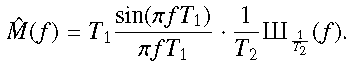 (2)The product of a signal and a Dirac comb is equivalent to a sampling. Thus, the convolution by a regular window function causes a spectral leakage from the main lobe to the side lobes that are regularly spaced in frequency by
  and their heights are modulated by the sinc term. This window effect depends on both T1 and T2.
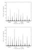 |
Fig. 1 Power density spectrum (in units of ppm2/μHz) of VIRGO/SPM data in the frequency range between 2700 to 3500 μHz estimated with a fast Fourier transform from a complete time series of 50 days (top) and 91.2 days (bottom). |
For this study, we use the time series obtained by the SunPhotometers (SPM) of VIRGO (Variability of Solar Irradiance and Gravity Oscillations, Fröhlich et al. 1995) instrument onboard the SoHO spacecraft (with a duty cycle close to 100%) in order to mimic ground-based observations. We only considered 50 days of observations in order to be close to what we expect for a typical long observation run with the SONG network. This is our ideal time series X(t). The top panel of Fig. 1 shows the power density spectrum (PDS) estimated from 50 days observations with a complete time coverage (duty cycle of 100%). We only plotted the PDS in the frequency range between 2700 to 3500 μHz to focus around the maximum power of the p modes. For this simple case, with regularly sampled data, without gaps, the spectrum was computed using a fast Fourier transform and we normalized it as the so-called one-sided PDS (Press et al. 1992).
3.1. Ground-based observations of single- to multiple-site networks: worst-case scenario
We started by studying the impact of different standard window functions from ground-based observations that have different duty cycles. To do so, we applied three different window functions to the VIRGO/SPM data.
To study the case of ground-based observations from a single site, we expanded the MARK-I window function to simulate a duty cycle of 23%. MARK-I is one of the helioseismic Doppler-velocity instruments of the BiSON network operated at the Observatorio del Teide, Tenerife (Chaplin et al. 1998), and located close to the first SONG node. This window function is therefore a reasonable approximation of what the observations with one node will have during its operation. We applied a dilatation operator (i.e., an operator that enlarges the regions where information is provided) to the MARK-I window function to simulate the case of ground-based observations from two different sites with a duty cycle of 50%. Although this mask is not typical of real data, it contains highly periodic gaps. This allows us to test our algorithm in the worst-case scenario and to establish a lower limit of any improvement in the inpainting algorithm compared to CLEAN. Finally, a mask for a multiple-site network is obtained by inverting the MARK-I window function providing a duty cycle of 77%. Although day-time and night-time observations are not the same and instruments are different, these artificial regular masks are representative enough for ground-based network observations for us to reasonably compare the different methods, these artificial regular masks represent the worst-case scenario for ground-based observations, because they have a large number of regular gaps. The time series X is then multiplied by these observational window functions M to obtain the artificial observed data Y (see Fig. 2).
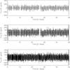 |
Fig. 2 Sample of 50 days of the original VIRGO/SPM data multiplied by a MARK-I like mask to simulate ground-based observations from a single site corresponding to a duty cycle of 23% (top panel), two different sites with a duty cycle of 50% (middle panel), and multiple sites corresponding to a duty cycle of 77% (bottom panel). |
These sets of data were then analyzed with the three methods described in Sect. 2. A comparison with linear interpolation for gap filling was shown in previous work, based on CoRoT data, which concluded that the inpainting method was superior (Sato et al. 2010). Nevertheless, we have applied the linear interpolation to the sets of simulated ground-based data described above, and the results are much poorer than the results with the three methods described in this paper.
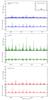 |
Fig. 3 Power density spectrum (in units of ppm2/μHz) for a duty cycle of 23%. The PDS is calculated with a least-squares sinewave fit on the incomplete time series (top panel), using an FFT on the CLEANed time series (middle panel) and an FFT on the inpainted time series (bottom panel). The errors correspond to the difference between the original PDS and the PDS estimated from the incomplete data. The inset corresponds to the spectral window of the time series. |
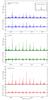 |
Fig. 4 Power density spectrum and errors (in units of ppm2/μHz) estimated from a time series of 50 days with a duty cycle of 50%. The PDS is computed with a least-squares sinewave fit on the incomplete time series (top panel), using an FFT on the CLEANed time series (middle panel) and an FFT on the inpainted time series (bottom panel). |
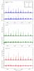 |
Fig. 5 Power density spectrum and errors (in units of ppm2/μHz) estimated from a time series of 50 days with a duty cycle of 77%. The PDS is computed with a least-squares sinewave fit on the incomplete time series (top panel), using an FFT on the CLEANed time series (middle panel) and an FFT on the inpainted time series (bottom panel). |
The PDSs obtained with the three methods described in Sect. 2 are shown in Figs. 3–5 for duty cycles of 23%, 50%, and 77%, respectively. In the top panel, the PDS is calculated by the method described in Frandsen et al. (1995), which consists of a least-squares sinewave fit (SWF) to the incomplete data where data points in the gaps are removed from the time series. In the middle panel, the PDS is obtained using a fast Fourier transform on a time series reconstructed using the CLEAN algorithm. The bottom panel presents the PDS computed with a fast Fourier transform after performing an inpainting. Each panel includes two plots: the PDS (top) and the error on the PDS (bottom). The plotted error corresponds to the difference between the power spectrum estimated from the complete data and the power spectrum estimated from the incomplete set. Thus positive errors correspond to underestimation of the signal. The magenta dotted lines have been plotted as a reference, and they correspond to an error of ±0.01 ppm2/μHz.
For a duty cycle of 23%, when using the SWF (top panel of Fig. 3) the oscillation modes are convolved by the Fourier transform of the mask, shown in the inset. The amplitude of the oscillation modes is substantially underestimated because of the spectral leakage1 of the power into the high amplitude side lobes of the spectral window. As a result, there are several spurious peaks, which correspond to negative values in the PDS error. This leakage is reduced when we increase the duty cycle (thus T1) as expected by Eq. (2), but the spurious peaks are still present in the PDS (top panels of Figs. 4 and 5).
With the CLEAN algorithm (middle panel of Fig. 3), we can see the improvement compared to the least-squared sinewave fit. The amplitude of the main high peaks is closer to the original PDS, and the side lobes have been reduced compared to the previous method. However, there are still some side lobes in the power spectrum that correspond to incorrect removal of the peaks. Because of the regularity of the mask, we are in the “worst case scenario” for the CLEAN algorithm, which looks in an iterative way for the highest peaks in the PDS, assuming they are due to real signal. As seen in Fig. 3, the amplitude of the side lobes is very close to the amplitude of the main lobe, so two side lobes from two nearby main lobes can be larger than the main lobes. This explains the side lobes that remain in the power spectrum. With duty cycles of 50% and 77% (middle panels of Figs. 4 and 5), the side lobes are significantly reduced as for the SWF method, but there is still a small spectral leakage even at the 77% duty cycle.
Like CLEAN, applying the inpainting method to the data with 23% duty cycle (bottom panel of Fig. 3) shows a clear reduction in the side lobes compared to SWF, but the amplitude of the peaks is not recovered well. However, there are a few instances where the main peaks are almost completely missed (see large positive peaks in the PDS error plots). These errors are due to the mask not satisfying one of the principal conditions previously laid down: “mask has to be sufficiently random”. Also for inpainting this is the “worst case scenario”, because the amount of missing data is significant, and the mask is coherent. Even worse, because the mask is regular, it is sparse in the representation ΦT of the data (i.e. multiscale discrete cosine transform) in which the signal is also sparse. In this case, the effect of the window function cannot be fully removed. The increase in the duty cycle to 50% and 77% (bottom panels of Figs. 4 and 5) improves the results of the inpainting method where we clearly see the reduction of the side lobes. We also notice that the amplitudes of the main peaks are recovered much better.
In summary, the CLEAN method is better at estimating the amplitude of the modes for typical ground-based data with duty cycles of 23%, while the inpainting method removes the side lobes better than CLEAN does for the 50% and 77% cases.
Fitted parameters: frequency (ν), rms amplitude (σrms), and width (Γ) of modes l = 0 to 3 of five radial orders around νmax.
3.2. Fitting the acoustic modes of the different power density spectra
In the case of a 23% duty cycle, the inpainting method is clearly not optimal for processing the regularly gapped ground-based data, but for a duty cycle of 77%, the inpainting method outperforms the other methods. To further quantify the results obtained in the intermediate case of 50% duty cycle, we fit the oscillation modes with a maximum likelihood estimation as described in Anderson et al. (1990) and Appourchaux et al. (1998). Modes are modeled as the sum of Lorentzian profiles (see, e.g., Kumar et al. 1988) and are fitted simultaneously over one large separation, i.e., a sequence of l = 2,0,3, and 1 modes, assuming a common width for the modes and a common rotational splitting (fixed to 0.4 μHz), and assuming that the Sun is observed from near the equatorial plane of the Sun (90° inclination). We fit five sequences of modes by fixing within each sequence the visibilities for l = 1,2,3 modes relatively to the l = 0 mode (see, e.g., Ballot et al. 2011, for details on fitting techniques).
In the PDS obtained by sinewave fitting, the amplitude of the modes is significantly underestimated due to leakage of the power into the side lobes of the spectral window. To minimize the effect of this spectral leakage, the fitted model is convolved with the spectral window.
The PDS reconstructed from the CLEAN method is hard to fit with this technique, since the statistics of the noise is modified in a non-trivial way. To avoid this problem, we would need to CLEAN the spectrum down to very low amplitude, which is too time-consuming.
Fitting results are reported in Table 1. We should remember that the errors are underestimated in the case of the PDS obtained by sinewave fitting, because the statistics used does not take the correlation between the points introduced by the window function into account. Except for l = 3 modes, we see that the mode parameters are recovered well in both cases. Nevertheless, we must be very cautious by interpreting such a table because it concerned only five modes for one given noise realization. Moreover, these results are obtained with good guesses, close to the real parameters. Fits of the PDS obtained by sinewave fitting are very sensitive to the guesses because of the presence of day aliases. This problem is avoided when the series are inpainted for which side lobes are strongly reduced.
4. Application to realistic simulations of space-based data
Space-based observations, in particular those by CoRoT and Kepler, have duty cycles around 90%. However, even small gaps on the time series can introduce significant artifacts into the power spectrum if they are regularly distributed.
4.1. CoRoT-like data
The CoRoT mission provides three to five month-long observations of high-precision photometry. However, these time series are periodically perturbed by high-energy particles hitting the satellite when crossing the South Atlantic Anomaly (SAA; e.g., Auvergne et al. 2009), resulting in gaps in the data. The gaps in the CoRoT light curves have a typical time duration of 20 min and a periodicity that comes from the orbital period of the satellite. Fortunately, even if the satellite is crossing the SAA regularly, the perturbation is not the same for each orbit. Thus, the observational window of CoRoT is more complex and cannot be easily modeled. We can still estimates the spectral window using a fast Fourier transform. The inset in the top panel of Fig. 6 shows a typical spectral window of CoRoT. There is about 15% of the power that leaks from the main lobe into the side lobes. However, in contrast to the previous masks, the side lobes are not significant. In this case, only 0.1% of the amplitude leaks into the first side lobes because the power is spread into more frequencies. It would be 3%, if the mask was regular.
4.1.1. Oscillation modes
In this section, we study the impact of these small repetitive gaps on the detection and estimation of the oscillation modes. For this purpose, we consider the observation window of the star HD 169392 (Mathur et al. 2013a), which was observed by CoRoT over 91.2 continuous days during the third long-run in the galactic center direction with a duty cycle of 83.4% and with a sampling of 32 s. This window is applied to 91.2 days of VIRGO data in which the original CoRoT 32 s cadence has been converted into the 60 s cadence of VIRGO data. The bottom panel of Fig. 1 shows the power density spectrum (PDS) estimated from 91.2 days of observations with a complete time coverage (duty cycle of 100%).
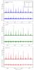 |
Fig. 6 Power density spectrum and errors (in units of ppm2/μHz) estimated from a time series of 91.2 days masked with a mask of CoRoT corresponding to a duty cycle of 83.4%. The PDS is computed with a least-squares sinewave fit on the incomplete time series (top panel), using an FFT on the CLEANed time series (middle panel) and an FFT on the inpainted time series (bottom panel). |
Figure 6 shows the results for this CoRoT-like data following the previous format. As expected from the shape of the window function in the Fourier domain (see inset), the side lobes have almost disappeared from the PDS obtained by sinewave fitting. However, there is still a small spectral leakage of the power into the side lobes as said previously. The PDS estimated from CLEAN yields a good estimation of the amplitude of the oscillation modes and the side lobes have almost disappeared. This is due to the observation window that produces a low level of side lobes, that helps the CLEAN algorithm to avoid detecting false peaks. Once more, there is a significant improvement in estimation of the amplitude of the oscillation modes for the inpainted data. This is certainly due to the random way in which the high-energy particles hit the satellite. This insures a given amount of incoherence to the mask despite the regularity with which the satellite crosses the SAA area.
4.1.2. Background power spectrum
Again, we study the impact of the small repetitive gaps induced by the SAA crossing on the power spectrum estimation. However, this time we focus on the background part of the power spectrum rather than the oscillation modes. In addition to the oscillation modes, the asteroseismic observations allow us to measure the stellar granulation signature by the characterization of the background power spectrum (Mathur et al. 2011). The spectral signature of granulation is expected to reveal time scales that are characteristic of the convection process in the stars. However, this analysis requires that we estimate the full power spectrum.
For this study, the CLEAN algorithm has not been considered because it is very time-consuming to reconstruct the full power spectrum as explained in Sect. 4.1.3.
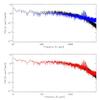 |
Fig. 7 Power density spectrum smoothed with a 4-point boxcar function (in units of ppm2/μHz) estimated from a time series of 24 days of VIRGO/SPM masked with a mask of CoRoT with a duty cycle of 70%. The black curve corresponds to the original PDS estimated from the complete data. In the top panel, the blue curve corresponds to the PDS calculated with a least-squares sinewave fit on the incomplete data. Bottom panel, the red curve correspond to the PDS estimated using a fast Fourier transform on the inpainted data. |
The top panel of Fig. 7 shows the original PDS of VIRGO/SPM estimated from the complete data compared to a PDS estimated from the incomplete data. We can see that the level of power at high frequencies is overestimated, resulting in a bad granulation characterization. Moreover, the increase in the high-frequency noise affects the oscillation modes at high frequency (Jiménez et al. 2011), as well as the pseudo-mode region (García et al. 1998). In the bottom panel of Fig. 7, we show the power spectrum estimated after inpainting of the data, and it appears that the inpainting technique recovers the high-frequency level of the power spectrum better.
To quantify the difference between the backgrounds of the different PDS, we fit them with the following model: ![Mathematical equation: \begin{eqnarray} \label{eq:bg} B(\nu) &=& \frac{\zeta_{\mathrm{g}}\sigma^2_{\mathrm{g}}}{1+(2\pi\tau_{\mathrm{g}}\nu)^{3.5}} + \frac{\zeta_{\mathrm{f}}\sigma^2_{\mathrm{f}}}{1+(2\pi\tau_{\mathrm{f}}\nu)^{6.2}} \nonumber \\ &&+\exp \left[-\frac{(\nu-\nu_{\rm o})^2}{2\delta_{\rm o}^2}\right] + W. \end{eqnarray}](/articles/aa/full_html/2015/02/aa22361-13/aa22361-13-eq164.png) (3)The first two terms are Harvey profiles. The first component is modeling the granulation, and it is parametrized with τg, the characteristic time scale of the granulation, σg its rms amplitude and ζg = 2.73 is a normalization factor. The second component, possibly originating in faculae, is parametrized with τf and σf. The normalization factor is ζf = 3.00. The exponents 3.5 and 6.2 are chosen according to Karoff (2012). The third component is a Gaussian function parametrized with νo and δo to account for the power excess due to oscillation modes. Finally, W is the white noise component. Spectra are fitted using a maximum likelihood estimation between 100 μHz and the Nyquist frequency, by assuming that the noise follows a
(3)The first two terms are Harvey profiles. The first component is modeling the granulation, and it is parametrized with τg, the characteristic time scale of the granulation, σg its rms amplitude and ζg = 2.73 is a normalization factor. The second component, possibly originating in faculae, is parametrized with τf and σf. The normalization factor is ζf = 3.00. The exponents 3.5 and 6.2 are chosen according to Karoff (2012). The third component is a Gaussian function parametrized with νo and δo to account for the power excess due to oscillation modes. Finally, W is the white noise component. Spectra are fitted using a maximum likelihood estimation between 100 μHz and the Nyquist frequency, by assuming that the noise follows a  distribution.
Table 2 shows the results of the fitting. In the spectrum obtained with the sinewave fitting, the Harvey parameters are badly fit. By contrast, the inpainted spectrum allows us to correctly recover both the amplitude and the characteristic time scale for the two components. The main visible change is an increase in the white noise component, generated by an increase in the high frequency noise. However, this excess of high frequency noise remains small compared to the SWF case.
4.1.3. Processing time
For space-based data for which we have to deal with long and continuous observations, the impact of the gaps is less, because the duty cycle is approaching 100%. For this reason, the way the missing data are handled is frequently driven by the time it takes to do the correction.
We have estimated the processing time for the three methods used in this paper:
-
The SWF has a time complexity of O(N2) where N is the number of datapoints of the time series. This time complexity can be reduced to O(NNf) ifwe are just interested in reconstructing a number offrequencies Nf.
-
The CLEAN algorithm has a time complexity of O(N3). In the same way, it can be reduced to
 if we are just interested in a part of the power spectrum. This scaling means that for long time series, this algorithm may prove to be very time-consuming.
 -
The inpainting algorithm has a time complexity of O(ImaxNlog (N)). The number of iterations Imax is taken as equal to 100.
For a time series of 50 days observed with a sampling of 32 s, which is the case for the CoRoT long-cadence observations, with a duty cycle of about 77%, it takes four hours to compute one tenth of the full SWF power spectrum up to the Nyquist frequency, about four days to compute one tenth of the CLEAN power spectrum and only 4 min to compute the full inpainted power spectrum on a 2 × 2.4 GHz Intel Xeon Quad-Core processor. Thus, even considering just a fraction of the power spectrum, the inpainting algorithm is 1000 times faster than the CLEAN algorithm and 60 times faster than the SWF method.
4.2. Kepler-like data
Since its launch in May 2009, NASA’s Kepler mission (Borucki et al. 2010) has also been used to study stars with asteroseismology. Indeed, around 2000 solar-like stars (Chaplin et al. 2011) have been observed continuously in short cadence – with a sampling rate of ~58.85 s (see for details, Gilliland et al. 2010b; García et al. 2011) – for at least one month and up to two years. In addition, around 15 000 red giants showing solar-like oscillations have been observed in long cadence (sampling of ~29.5 min) (e.g., Bedding et al. 2010; Huber et al. 2011; Stello et al. 2013).
Kepler data typically reach duty cycles of about 93%, where gaps are mainly due to a combination of data downlinks (of around one day in average) every three months and desaturations (of one long-cadenced data point and several short-cadenced data points) every three days (Christiansen et al. 2013).
Owing to their regularity, these single-point gaps produce a similar effect at high frequencies to those shown for CoRoT in Fig. 7, which is the most pronounced for stars showing high-amplitude modulation at low frequencies. By only inpainting the single long-cadence point missing every three days, we could thus almost completely remove the spectral leakage of power at high frequencies in the Kepler data.
4.2.1. Irregularly sampled data
The inpainting algorithm has not yet been developed for irregularly sampled data, such as Kepler data, because the multiscale discrete cosine transform that is used assumes regularly sampled data. Therefore, before applying the algorithm, we place the irregularly Kepler data into a regular grid using the nearest-neighbor resampling algorithm (Broersen 2009). We therefore built a new time series with a sampling rate equal to the median of the original. Each point in the new series is built from the closest observation (irregularly sampled) if it is within half of the new sampling distance. The regular grid point is set to zero if there is no original observation falling within the new grid (for further details see García et al. 2014).
5. Conclusions
All improvements in the gap-filling data are of special importance for analyzing asteroseismology data. We have shown in this paper that CLEAN and inpainting are efficient methods for dealing with gaps in ground-based and spaced-based data. Both CLEAN and inpainting methods are based on iterative algorithms that try to deconvolve the observed time series from the window function. However, the difference comes from the way the deconvolution is conducted. In the CLEAN algorithm, a direct deconvolution is performed for each frequency. In the inpainting algorithm, the window function is deconvolved indirectly by filling in the gaps.
We showed that CLEAN allows us to process ground-based data with low duty cycles (lower than 50%) more efficiently than the inpainting method because it recovers the amplitudes of the modes better. In addition, these low duty cycle time series can be tackled with a reasonable amount of time by CLEAN that removes the data points from the gaps. For duty cycles higher than 50%, the inpainting becomes more interesting. It provides similar and even slightly better results than CLEAN but for a much shorter computational time. Indeed for 50 day-time series with a sampling of 32 s and a duty cycle of 77%, it is about 1000 times faster than CLEAN.
For data with higher duty cycles as is typical of space-based observations, the inpainting algorithm retrieves the modes better and becomes a powerful tool that we can apply to thousands of stars in a short amount of time. This is very important in the framework of the Kepler mission that provided very long time series (around 4 years) for hundreds of thousands of stars covering the HR diagram (e.g., Gilliland et al. 2010a).
Finally, we showed that it is important to fill the gaps of the data to better characterize the background at high frequency, as well as the granulation components, which are very affected. Given the computation time factor, the choice of the method would lean toward the inpainting because it would be much more time-consuming to compute the whole power spectrum with CLEAN.
The Kepler Asteroseismic Scientific Consortium has developed its own automated correction software (García et al. 2011) to correct most of the light curves with a minimum human intervention. As a result of this study, the inpainting technique has been added to the pipeline to improve the asteroseismic studies. Furthermore, the inpainting software presented in this study is now publicly available2.
The spectral leakage caused by the window function is sometimes called incorrectly aliasing. Aliasing should only be used if the spectral leakage is caused by sampling.
The Kepler-inpainting software can be found in http://irfu.cea.fr/Sap/en/Phocea/Vie_des_labos/Ast/ast_visu.php?id_ast=3346
Acknowledgments
The research leading to these results has received funding from the European Community’s Seventh Framework Program (FP7/2007-2013) under grant agreement no. 269194 (IRSES/ASK) and ERC-228261 (SparseAstro). R.A.G., S.M., and S.P. acknowledge the School of Physics staff of the University of Sydney for their warm hospitality during the IRSES research program. S.M. thanks the University of Sydney for their travel support. NCAR is partially funded by the National Science Foundation. This work was partially supported by the NASA grant NNX12AE17G.
References
- Abrial, P., Moudden, Y., Starck, J.-L., et al. 2008, Stat. Methodol., 5, 289 [Google Scholar]
- Anderson, E. R., Duvall, Jr., T. L., & Jefferies, S. M. 1990, ApJ, 364, 699 [NASA ADS] [CrossRef] [Google Scholar]
- Appourchaux, T., Gizon, L., & Rabello-Soares, M.-C. 1998, A&AS, 132, 107 [NASA ADS] [CrossRef] [EDP Sciences] [Google Scholar]
- Appourchaux, T., Michel, E., Auvergne, M., et al. 2008, A&A, 488, 705 [NASA ADS] [CrossRef] [EDP Sciences] [Google Scholar]
- Auvergne, M., Bodin, P., Boisnard, L., et al. 2009, A&A, 506, 411 [NASA ADS] [CrossRef] [EDP Sciences] [Google Scholar]
- Baglin, A., Auvergne, M., Barge, P., et al. 2006, in ESA SP, eds. M. Fridlund, A. Baglin, J. Lochard, & L. Conroy, 1306, 33 [Google Scholar]
- Ballot, J., Gizon, L., Samadi, R., et al. 2011, A&A, 530, A97 [NASA ADS] [CrossRef] [EDP Sciences] [Google Scholar]
- Beck, P. G., Montalban, J., Kallinger, T., et al. 2012, Nature, 481, 55 [NASA ADS] [CrossRef] [Google Scholar]
- Bedding, T. R., Huber, D., Stello, D., et al. 2010, ApJ, 713, L176 [NASA ADS] [CrossRef] [Google Scholar]
- Benomar, O., Baudin, F., Campante, T. L., et al. 2009, A&A, 507, L13 [NASA ADS] [CrossRef] [EDP Sciences] [Google Scholar]
- Borucki, W. J., Koch, D., Basri, G., et al. 2010, Science, 327, 977 [NASA ADS] [CrossRef] [PubMed] [Google Scholar]
- Broersen, P. M. T. 2009, IEEE Trans. Instr. Meas., 58, 1380 [CrossRef] [Google Scholar]
- Buzasi, D. L., Bruntt, H., Preston, H. L., & Clausen, J. V. 2004, in AAS Meeting Abstracts, BAAS, 36, 1369 [NASA ADS] [Google Scholar]
- Chaplin, W. J., Elsworth, Y., Howe, R., et al. 1996, Sol. Phys., 168, 1 [Google Scholar]
- Chaplin, W. J., Elsworth, Y., Isaak, G. R., et al. 1998, MNRAS, 300, 1077 [NASA ADS] [CrossRef] [Google Scholar]
- Chaplin, W. J., Kjeldsen, H., Christensen-Dalsgaard, J., et al. 2011, Science, 332, 213 [NASA ADS] [CrossRef] [PubMed] [Google Scholar]
- Chaplin, W. J., Basu, S., Huber, D., et al. 2014, ApJS, 210, 1 [NASA ADS] [CrossRef] [Google Scholar]
- Christensen-Dalsgaard, J., Dappen, W., Ajukov, S. V., et al. 1996, Science, 272, 1286 [CrossRef] [Google Scholar]
- Christiansen, J., Jenkins, J., Caldwell, D., et al. 2013, Kepler Data Characteristics Handbook (KSCI-19040-004) [Google Scholar]
- Deheuvels, S., Bruntt, H., Michel, E., et al. 2010, A&A, 515, A87 [NASA ADS] [CrossRef] [EDP Sciences] [Google Scholar]
- Deheuvels, S., García, R. A., Chaplin, W. J., et al. 2012, ApJ, 756, 19 [NASA ADS] [CrossRef] [Google Scholar]
- Donoho, D., & Elad, M. 2003, PNAS, 100, 2197 [Google Scholar]
- Donoho, D., & Huo, X. 2001, IEEE Transactions on Information Theory, 47, 2845 [Google Scholar]
- Doğan, G., Metcalfe, T. S., Deheuvels, S., et al. 2013, ApJ, 763, 49 [NASA ADS] [CrossRef] [Google Scholar]
- Elad, M., & Bruckstein, A. 2002, IEEE Transactions on Information Theory, 48, 2558 [CrossRef] [Google Scholar]
- Elad, M., Starck, J.-L., Querre, P., & Donoho, D. 2005, Journal on Applied and Computational Harmonic Analysis, 19, 340 [Google Scholar]
- Fahlman, G. G., & Ulrych, T. J. 1982, MNRAS, 199, 53 [NASA ADS] [CrossRef] [Google Scholar]
- Ferraz-Mello, S. 1981, AJ, 86, 619 [NASA ADS] [CrossRef] [Google Scholar]
- Fletcher, S. T., Chaplin, W. J., Elsworth, Y., Schou, J., & Buzasi, D. 2006, MNRAS, 371, 935 [NASA ADS] [CrossRef] [Google Scholar]
- Foster, G. 1995, AJ, 109, 1889 [NASA ADS] [CrossRef] [Google Scholar]
- Frandsen, S., Jones, A., Kjeldsen, H., et al. 1995, A&A, 301, 123 [NASA ADS] [Google Scholar]
- Fröhlich, C., Romero, J., Roth, H., et al. 1995, Sol. Phys., 162, 101 [NASA ADS] [CrossRef] [Google Scholar]
- Gabriel, A. H., Grec, G., Charra, J., et al. 1995, Sol. Phys., 162, 61 [NASA ADS] [CrossRef] [Google Scholar]
- García, R. A., Palle, P. L., Turck-Chieze, S., et al. 1998, ApJ, 504, L51 [NASA ADS] [CrossRef] [Google Scholar]
- García, R. A., Turck-Chièze, S., Boumier, P., et al. 2005, A&A, 442, 385 [NASA ADS] [CrossRef] [EDP Sciences] [Google Scholar]
- García, R. A., Régulo, C., Samadi, R., et al. 2009, A&A, 506, 41 [NASA ADS] [CrossRef] [EDP Sciences] [Google Scholar]
- García, R. A., Mathur, S., Salabert, D., et al. 2010, Science, 329, 1032 [NASA ADS] [CrossRef] [PubMed] [Google Scholar]
- García, R. A., Hekker, S., Stello, D., et al. 2011, MNRAS, 414, L6 [NASA ADS] [CrossRef] [Google Scholar]
- García, R. A., Mathur, S., Pires, S., et al. 2014, A&A, 568, A10 [NASA ADS] [CrossRef] [EDP Sciences] [Google Scholar]
- Gilliland, R. L., Brown, T. M., Christensen-Dalsgaard, J., et al. 2010a, PASP, 122, 131 [NASA ADS] [CrossRef] [Google Scholar]
- Gilliland, R. L., Jenkins, J. M., Borucki, W. J., et al. 2010b, ApJ, 713, L160 [NASA ADS] [CrossRef] [Google Scholar]
- Gizon, L., Ballot, J., Michel, E., et al. 2013, PNAS, 110, 13267 [NASA ADS] [CrossRef] [Google Scholar]
- Grundahl, F., Kjeldsen, H., Frandsen, S., et al. 2006, Mem. Soc. Astron. Italiana, 77, 458 [Google Scholar]
- Harvey, J. W., Hill, F., Hubbard, R. P., et al. 1996, Science, 272, 1284 [NASA ADS] [CrossRef] [PubMed] [Google Scholar]
- Huber, D., Bedding, T. R., Stello, D., et al. 2011, ApJ, 743, 143 [NASA ADS] [CrossRef] [Google Scholar]
- Jiménez, A., García, R. A., & Pallé, P. L. 2011, ApJ, 743, 99 [NASA ADS] [CrossRef] [Google Scholar]
- Karoff, C. 2012, MNRAS, 421, 3170 [NASA ADS] [CrossRef] [Google Scholar]
- Karoff, C., Campante, T. L., Ballot, J., et al. 2013, ApJ, 767, 34 [NASA ADS] [CrossRef] [Google Scholar]
- Kumar, P., Franklin, J., & Goldreich, P. 1988, ApJ, 328, 879 [NASA ADS] [CrossRef] [Google Scholar]
- Larson, T. P., & Schou, J. 2008, J. Phys. Conf. Ser., 118, 2083 [Google Scholar]
- Lomb, N. R. 1976, Ap&SS, 39, 447 [NASA ADS] [CrossRef] [Google Scholar]
- Mathur, S., Hekker, S., Trampedach, R., et al. 2011, ApJ, 741, 119 [NASA ADS] [CrossRef] [Google Scholar]
- Mathur, S., Metcalfe, T. S., Woitaszek, M., et al. 2012, ApJ, 749, 152 [NASA ADS] [CrossRef] [Google Scholar]
- Mathur, S., Bruntt, H., Catala, C., et al. 2013a, A&A, 549, A12 [CrossRef] [EDP Sciences] [Google Scholar]
- Mathur, S., García, R. A., Morgenthaler, A., et al. 2013b, A&A, 550, A32 [NASA ADS] [CrossRef] [EDP Sciences] [Google Scholar]
- Metcalfe, T. S., Chaplin, W. J., Appourchaux, T., et al. 2012, ApJ, 748, L10 [NASA ADS] [CrossRef] [Google Scholar]
- Mosser, B., Michel, E., Appourchaux, T., et al. 2009, A&A, 506, 33 [NASA ADS] [CrossRef] [EDP Sciences] [Google Scholar]
- Mosser, B., Goupil, M. J., Belkacem, K., et al. 2012, A&A, 548, A10 [NASA ADS] [CrossRef] [EDP Sciences] [Google Scholar]
- Pires, S., Starck, J.-L., Amara, A., et al. 2009, MNRAS, 395, 1265 [NASA ADS] [CrossRef] [Google Scholar]
- Press, W. H., Teukolsky, S. A., Vetterling, W. T., & Flannery, B. P. 1992, Numerical recipes in C. The art of scientific computing (Cambridge University Press) [Google Scholar]
- Roberts, D. H., Lehar, J., & Dreher, J. W. 1987, AJ, 93, 968 [NASA ADS] [CrossRef] [Google Scholar]
- Sato, K. H., García, R. A., Pires, S., et al. 2010, in Proc. of the HELAS IV International Conf. [Google Scholar]
- Scargle, J. D. 1982, ApJ, 263, 835 [NASA ADS] [CrossRef] [Google Scholar]
- Scherrer, P. H., Bogart, R. S., Bush, R. I., et al. 1995, Sol. Phys., 162, 129 [Google Scholar]
- Scherrer, P. H., Schou, J., Bush, R. I., et al. 2012, Sol. Phys., 275, 207 [Google Scholar]
- Starck, J.-L., & Murtagh, F. 2002, Astronomical image and data analysis (Berlin: Springer) [Google Scholar]
- Stello, D., Huber, D., Bedding, T. R., et al. 2013, ApJ, 765, L41 [NASA ADS] [CrossRef] [Google Scholar]
- Walker, G., Matthews, J., Kuschnig, R., et al. 2003, PASP, 115, 1023 [NASA ADS] [CrossRef] [Google Scholar]
- Zechmeister, M., & Kürster, M. 2009, A&A, 496, 577 [NASA ADS] [CrossRef] [EDP Sciences] [Google Scholar]
All Tables
Fitted parameters: frequency (ν), rms amplitude (σrms), and width (Γ) of modes l = 0 to 3 of five radial orders around νmax.
All Figures
|
Fig. 1 Power density spectrum (in units of ppm2/μHz) of VIRGO/SPM data in the frequency range between 2700 to 3500 μHz estimated with a fast Fourier transform from a complete time series of 50 days (top) and 91.2 days (bottom). |
| In the text | |
|
Fig. 2 Sample of 50 days of the original VIRGO/SPM data multiplied by a MARK-I like mask to simulate ground-based observations from a single site corresponding to a duty cycle of 23% (top panel), two different sites with a duty cycle of 50% (middle panel), and multiple sites corresponding to a duty cycle of 77% (bottom panel). |
| In the text | |
|
Fig. 3 Power density spectrum (in units of ppm2/μHz) for a duty cycle of 23%. The PDS is calculated with a least-squares sinewave fit on the incomplete time series (top panel), using an FFT on the CLEANed time series (middle panel) and an FFT on the inpainted time series (bottom panel). The errors correspond to the difference between the original PDS and the PDS estimated from the incomplete data. The inset corresponds to the spectral window of the time series. |
| In the text | |
|
Fig. 4 Power density spectrum and errors (in units of ppm2/μHz) estimated from a time series of 50 days with a duty cycle of 50%. The PDS is computed with a least-squares sinewave fit on the incomplete time series (top panel), using an FFT on the CLEANed time series (middle panel) and an FFT on the inpainted time series (bottom panel). |
| In the text | |
|
Fig. 5 Power density spectrum and errors (in units of ppm2/μHz) estimated from a time series of 50 days with a duty cycle of 77%. The PDS is computed with a least-squares sinewave fit on the incomplete time series (top panel), using an FFT on the CLEANed time series (middle panel) and an FFT on the inpainted time series (bottom panel). |
| In the text | |
|
Fig. 6 Power density spectrum and errors (in units of ppm2/μHz) estimated from a time series of 91.2 days masked with a mask of CoRoT corresponding to a duty cycle of 83.4%. The PDS is computed with a least-squares sinewave fit on the incomplete time series (top panel), using an FFT on the CLEANed time series (middle panel) and an FFT on the inpainted time series (bottom panel). |
| In the text | |
|
Fig. 7 Power density spectrum smoothed with a 4-point boxcar function (in units of ppm2/μHz) estimated from a time series of 24 days of VIRGO/SPM masked with a mask of CoRoT with a duty cycle of 70%. The black curve corresponds to the original PDS estimated from the complete data. In the top panel, the blue curve corresponds to the PDS calculated with a least-squares sinewave fit on the incomplete data. Bottom panel, the red curve correspond to the PDS estimated using a fast Fourier transform on the inpainted data. |
| In the text | |
Current usage metrics show cumulative count of Article Views (full-text article views including HTML views, PDF and ePub downloads, according to the available data) and Abstracts Views on Vision4Press platform.
Data correspond to usage on the plateform after 2015. The current usage metrics is available 48-96 hours after online publication and is updated daily on week days.
Initial download of the metrics may take a while.