| Issue |
A&A
Volume 573, January 2015
|
|
|---|---|---|
| Article Number | A119 | |
| Number of page(s) | 9 | |
| Section | Interstellar and circumstellar matter | |
| DOI | https://doi.org/10.1051/0004-6361/201424948 | |
| Published online | 08 January 2015 | |
Fragmentation and kinematics of dense molecular cores in the filamentary infrared-dark cloud G011.11–0.12⋆,⋆⋆
1
Max Planck Institute for Astronomy, Königstuhl 17, 69117
Heidelberg,
Germany
e-mail: This email address is being protected from spambots. You need JavaScript enabled to view it.
2
European Southern Observatory, Karl-Schwarzschild-Str. 2, 85748
Garching bei München,
Germany
Received: 8 September 2014
Accepted: 7 November 2014
Abstract
We present new Plateau de Bure Interferometer observations of a region in the filamentary infrared-dark cloud (IRDC) G011.11-0.12 containing young, star-forming cores. In addition to the 3.2 mm continuum emission from cold dust, we map this region in the N2H+(1−0) line to trace the core kinematics with an angular resolution of 2′′ and velocity resolution of 0.2 km s-1. These data are presented in concert with recent Herschel results, single-dish N2H+(1−0) data, SABOCA 350 μm continuum data, and maps of the C18O (2−1) transition obtained with the IRAM 30 m telescope. We recover the star-forming cores at 3.2 mm continuum, while in N2H+ they appear at the peaks of extended structures. The mean projected spacing between N2H+ emission peaks is 0.18 pc, consistent with simple isothermal Jeans fragmentation. The 0.1 pc-sized cores have low virial parameters on the criticality borderline, while on the scale of the whole region, we infer that it is undergoing large-scale collapse. The N2H+ linewidth increases with evolutionary stage, while CO isotopologues show no linewidth variation with core evolution. Centroid velocities of all tracers are in excellent agreement, except in the starless region where two N2H+ velocity components are detected, one of which has no counterpart in C18O. We suggest that gas along this line of sight may be falling into the quiescent core, giving rise to the second velocity component, possibly connected to the global collapse of the region.
Key words: stars: formation / ISM: kinematics and dynamics / submillimeter: ISM
Based on observations carried out with the IRAM Plateau de Bure Interferometer and the IRAM 30 m Telescope. IRAM is supported by INSU/CNRS (France), MPG (Germany) and IGN (Spain).
N2H+ data cube (in FITS format) is only available at the CDS via anonymous ftp to cdsarc.u-strasbg.fr (130.79.128.5) or via http://cdsarc.u-strasbg.fr/viz-bin/qcat?J/A+A/573/A119
© ESO, 2015
1. Introduction
If we are to understand the enrichment and evolution of galaxies and their interstellar medium (ISM), the conditions under which high-mass stars form is an essential component of any theory to get right. They dominate the stellar energy and momentum feedback, which in turn drives the chemistry and thermodynamic state of the ISM, and thus determine the properties of further generations of star formation.
Any theoretical model of high-mass star and cluster formation profoundly depends on the imposed initial conditions, thus it is of principle importance that observers diligently characterise the physical conditions of the earliest phases of the process on both large and small scales. All stars form in molecular clouds, confined to the densest regions within the clouds. In order for massive stars to form, a large amount of mass at relatively high concentration is required. The class of objects known as infrared-dark clouds (IRDCs), which appear in silhouette against the mid-infrared background of the Galaxy (Perault et al. 1996; Carey et al. 1998), have been identified as excellent hunting grounds for the precursors to high-mass star and cluster formation.
The target of our study is the filamentary IRDC G011.11−0.12 (henceforth G11). Based on the Reid et al. (2009) Galactic rotation curve model, we find a kinematic distance of 3.41 kpc to G11 (assuming a vlsr = 29.2 km s-1) and adopt it throughout this work. We note that this distance differs from the distance inferred from extinction studies which infer distances of 4.1 kpc (Kainulainen et al. 2011) and 4.7 kpc (Marshall et al. 2009). G11 was first found because of its remarkable absorbing contrast at 8 μm (Egan et al. 1998; see also Kainulainen et al. 2013) and carries on in absorption up to 100 μm (Henning et al. 2010). This massive (M(N> 1022 cm-2) ~ 20 000 M⊙) filament (projected length ~30 pc) exceeds the critical mass-per-unit length value for an isothermal cylinder (Ostriker 1964), though, as with most IRDCs, G11 appears to be dominated by non-thermal motions (Kainulainen et al. 2013). Herschel observations have also revealed a population of embedded protostellar cores following the dense centre of the filament. The continuum peak “P1” (Carey et al. 2000; Johnstone et al. 2003) is a site of active high-mass star formation (Pillai et al. 2006b; Gómez et al. 2011; Wang et al. 2014).
Figure 1a shows the Herschel 70 μm image first presented in Henning et al. (2010) with the region we selected for this study shown in a box. We chose this small region because it (a) appears relatively isolated from the feedback effects from the active massive star formation and (b) contained embedded cores of different inferred evolutionary stages (Ragan et al. 2012b). We present new observations with the Plateau de Bure Interferometer (PdBI) of both the 3.2 mm continuum and N2H+(1−0) hyperfine transition. In addition, a new IRAM 30 m map of the C18O 2 → 1 transition is presented as a probe of the more diffuse environment. The goal of this study is to explore how G11 has fragmented into core substructures and whether there are distinct dynamical signatures – in the dense or diffuse gas – tied to the core evolution.
The new observations and those drawn from the literature are described in more detail in Sect. 2. We discuss the morphological and kinematic properties of the dense cores in Sect. 3 and compare them to the environment probed by C18O in Sect. 4. We place our results in context with other studies of IRDCs in Sect. 5 and summarise in Sect. 6.
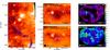 |
Fig. 1 a) Full G11 filament seen at 70 μm with Herschel/PACS with SPIRE 350 μm contours over-plotted from 9 Jy beam-1 increasing in steps of 3 Jy beam-1 (adapted from Henning et al. 2010). The SPIRE 350 μm beam (FWHM) is shown in the lower-left corner. The white rectangle marks the area shown in the rest of the panels. b) MIPS 24 μm image with 3.2 mm continuum contours from a PdBI-only map. The contour levels are from 0.2 to 0.12 mJy beam-1 in steps of 0.2 mJy beam-1. The synthesised beam is shown in the lower-left corner. c) APEX-SABOCA 350 μm continuum contours (Ragan et al. 2013) at 0.81, 1.08, 1.35 Jy beam-1 plotted over the PACS 100 μm image. The SABOCA 350 μm beam (FWHM) is shown in the lower left. d) Integrated intensity of N2H+ (1−0) from the PdBI-only map. e) Integrated intensity of the combined PdBI+MOPRA map. Both d) and e) are integrated from 29 to 33 km s-1, and the units of the colourscale are Jy beam-1km s-1. The + signs indicate the positions of the main continuum cores identified in panel b) and Table 1. |
2. Observations
2.1. IRAM Plateau de Bure: N2H+ 1 → 0
We observed a subregion of G11 (see Fig. 1) in a three-point mosaic with the Plateau de Bure Interferometer (PdBI) in the D (June 2010) and C configuration (November 2010), which covered projected baselines from 13 to 180 m as part of project U00D. We tuned to the 93.174 GHz transition of N2H+ (1−0) in the lower sideband and, simultaneously, the 13CS (2−1) transition at 92.494 GHz, which was not detected. Our spectral resolution is 0.2 km s-1. The maximum detectable source size is defined by the shortest baseline, λ/Dmin = 28′′, or 0.5 pc in G11.
The PdBI observations were reduced with the standard methods using the CLIC and MAPPING modules in the GILDAS software package1. We corrected for phase and amplitude fluctuations with frequent observations of J1830-210, J1832-206, and 3C 273, and the amplitude scale was set by observations of MWC 349 (Sν = 1.15 Jy).
Single-dish observations of the N2H+ (1−0) transition were obtained with MOPRA2 in a survey by Tackenberg et al.
(2014). The observations have a beam FWHM of
35 5
and velocity resolution of 0.11 km
s-1.
5
and velocity resolution of 0.11 km
s-1.
We combined the PdBI and MOPRA data within the GILDAS software package, using the UVSHORT task in natural weighting mode. The synthesised beam of the combined dataset is 7.21′′× 2.97′′ with a position angle of 6 degrees east of north. At the final velocity resolution of 0.2 km s-1, the 3σ rms is 15 mJy beam-1.
We reduced the data with the CLASS module of the GILDAS software package. We fit a low-order polynomial to the baseline of each spectra, and the spectra were then summed over the relevant regions. We implemented the hfs method to account for the hyperfine structure of the N2H+ (1−0) transition (e.g. Caselli et al. 1995).
2.2. IRAM 30-m: C18O 2 → 1
We observed the region in the C18O(2−1) transition at 219.560354 GHz with the IRAM 30-m telescope at Pico Veleta in Granada, Spain in January 2012 (project 172-11) in good conditions with less than 1 mm of precipitable water vapour. Pointing was checked with observations of 1757-240, and focus was performed on Mercury.
At this frequency, the telescope beam is 118.
Mapping was done in on-the-fly mode with position-switching, using a fixed OFF position
α2000 = 18:10:16.6, δ2000 =
−19:00:59.9. The HERA
receiver has 1 GHz bandwidth on the FFTS backend with which we achieved a velocity
resolution of 0.25 km
s-1 and 1σ rms of 200 mK in the
 scale. The data were reduced using the
CLASS module of the GILDAS software package. Spectral fits were made assuming a Gaussian
line profile after removing a first order baseline. These data are presented in full,
along with maps of the atomic and ionised carbon line transitions, in Beuther et al. (2014).
scale. The data were reduced using the
CLASS module of the GILDAS software package. Spectral fits were made assuming a Gaussian
line profile after removing a first order baseline. These data are presented in full,
along with maps of the atomic and ionised carbon line transitions, in Beuther et al. (2014).
2.3. Continuum studies
We incorporate multiple continuum measurements from previous studies to constrain the evolutionary stage of the cores in the region. Single-dish measurement at 850 μm with SCUBA shows that this region (box in Fig. 1a) contains ~700 M⊙ of gas mass (Henning et al. 2010). The Herschel (Pilbratt et al. 2010) guaranteed time key project entitled the Earliest Phases of Star Formation (EPoS: Henning et al. 2010; Ragan et al. 2012b) obtained maps at all PACS (Poglitsch et al. 2010) and SPIRE (Griffin et al. 2010) wavelengths of G11. The PACS data (see Fig. 1) in particular are sensitive to compact, protostellar cores embedded in the dense gas reservoir. We use these far-infrared data to infer the evolutionary stage of the various emission peaks depending on the characteristics of the spectral energy distribution (SED). Region 1 (Fig. 1, panel b) is infrared-dark through 160 μm, which signifies a very high column density and/or a lack of an internal heating source. Region 2 is dark at 24 μm, but bright at all PACS bands, which places it at a more advanced evolutionary stage than region 1. Region 3 is bright in all infrared bands, indicating that it is the most evolved source. The SEDs (λ≥ 70 μm) of the main cores in regions 2 and 3 were modelled with blackbody functions in Henning et al. (2010) resulting in temperatures of the “cold” core component (containing the bulk of the mass) of 19 and 21 K, respectively. With Herschel detections only at 100 and 160 μm, we placed an upper limit of 16 K on the temperature in region 1.
The SEDs of cores were revisited in Ragan et al.
(2013) with the addition of high-resolution
(78)
SABOCA data at 350 μm. Regions 1 and 3 were detected in the SABOCA maps,
while region 2 lacked sufficient signal-to-noise. The cores are of intermediate mass,
between 7 and 17 M⊙, and bolometric temperatures
(Tbol; Myers & Ladd 1993) progress from <13 K for region 1, 19 K and 37 K for regions 2 and 3,
respectively. The updated properties derived from SED fits are summarised in Table 1. For the calculations of masses and column densities,
we use the cold component temperatures of 13, 19 and 15 K for regions 1, 2 and 3,
respectively, from Ragan et al. (2013).
Simultaneously with the PdBI line observations, we obtained 3.2 mm continuum maps using
3.6 GHz effective bandwidth of the WideX correlator (Fig. 1b). The beam was 688
×
274,
and we achieved a 3σ sensitivity of 0.17 mJy beam-1 and detected regions 2
(α,
δ =
18h10m16.3s, −19°:24′:20.4″)
and 3 (α,
δ =
18h10m19.2s, −19°:24′:22.9″)
only. These regions have effective diameters of 7′′ and 11′′, respectively, in the continuum image.
Continuum properties of Herschel-identified regions.
3. Results: dense cores
3.1. Continuum emission
Figure 1 provides an overview of the G11 filament. Panel a shows the large-scale filament at 70 μm from our Herschel/PACS observations with SPIRE 350 μm contours overlaid (Ragan et al. 2012b). In panel b, we show the PdBI 3.2 mm continuum emission over the Spitzer/MIPS 24 μm image. The 3.2 mm continuum is detected toward 70 μm-bright regions 2 and 3, totalling 0.4 and 2.4 mJy, respectively. Following the standard assumptions3, we estimate masses from these continuum measurements, arriving at 3 and 17 M⊙ for regions 2 and 3, respectively. The error in the mass assumes the temperatures are good within 1 K (Ragan et al. 2012b) and does not account for uncertainty in the dust opacity. The latter can influence the mass estimate by up to a factor of two. We do not detect 3.2 mm continuum toward 70 μm-dark region 1 (3σ sensitivity of 0.17 mJy beam-1, corresponding to 1 M⊙). We note that if the extinction distance of 4.7 kpc were adopted, then the mass values would be about a factor of two higher.
For comparison, in Fig. 1c, we show the 350 μm SABOCA continuum emission (Ragan et al. 2013), which has similar angular resolution of 7.8′′ plotted over Herschel/PACS 100 μm data. Regions 1 and 3 are detected in the SABOCA map, and although 350 μm emission is seen near region 2, it is not a significant 3σ detection (rms = 0.27 Jy beam-1). The continuum properties are summarised in Table 1. Overall, the continuum selects the three bright peaks that had been identified with Herschel, while the N2H+ (1−0) emission (see Sect. 2.1) is more extended.
Cores and line parameters from PdBI-only and PdBI+MOPRA N2H+ (1−0) datasets.
3.2. N2H+ 1 → 0 emission
We show the integrated N2H+(1−0) emission in panels d (PdBI-only) and e (PdBI+MOPRA) of Fig. 1. In both, the N2H+ exhibits significantly more structure than the continuum. Infrared-identified regions 1 through 3 (see Sect. 2.3) lie at the peaks of extended structures in N2H+. We identify additional peaks in N2H+ integrated emission (e.g. denoted 1a, 1b, etc., in order of decreasing peak intensity) which were above our threshold of 0.75 Jy beam-1km s-1 in the combined dataset and list their offsets and spectral properties derived using the hfs method in the GILDAS package CLASS in Table 2.
We list the core diameters in Table 2 integrating out to where the N2H+ emission reaches the level of 0.75 Jy beam-1km s-1. The main regions (Table 1) have a projected separation of 0.45 pc (between region 1 and each of the other two regions). The N2H+ sub-cores (Table 2) exhibit a mean nearest neighbour separation of 0.18 pc (0.25 pc if we had assumed distance of 4.7 kpc). We note that the Jeans fragmentation length (0.2 pc assuming 104 cm-3, 12 K media) is only marginally resolved by our PdBI observations (0.12 pc × 0.05 pc).
The cores have a mean N2H+ column density of 7 × 1012 cm-2 over their areas and vary by less than a factor of two. Likewise, the [N2H+/H2] abundance is roughly 5 × 10⁻¹⁰ (using N(H2) from Table 1) in rough agreement with results from both nearby cores (e.g. Caselli et al. 2002; Tafalla et al. 2004; Tobin et al. 2013; Miettinen & Offner 2013) and more massive IRDC regions (e.g. Ragan et al. 2006; Beuther & Henning 2009; Vasyunina et al. 2011; Sanhueza et al. 2013; Gerner et al. 2014; Henshaw et al. 2014).
3.3. Velocity structure
The spectrum at each peak position was fit using the PdBI-only data as well as the combined data cube. The parameters are listed in Table 2. While the inclusion of the single-dish MOPRA data does not alter the centroid velocities beyond the measurement error (except for core 3d), the linewidths in the combined data cube are always larger than the PdBI-only data cube by at least 20% and up to factor of 3, due to the larger beam of the single-dish observations.
In Fig. 2, we show the N2H+ spectra extracted at each peak position from the combined (PdBI+MOPRA) data cube. The line intensities, velocities and linewidths are given in each panel and in Table 2. The strongest emission originates from the 24 μm-bright source 3a. Most peaks are well-fit with a single velocity component. A notable exception is 1a, which clearly requires two velocity components for a satisfactory fit. The stronger component is centred near the common velocity of the other cores, 29.7 km s-1, but there is a second component centred at 32.0 km s-1. This is also seen in Fig. 3, which is the channel map of the N2H+ (1−0) emission from the PdBI+MOPRA merged data cube. The steps in velocity are 0.6 km s-1. Interestingly, Core 1b exhibits a single velocity component, but nearer to the offset velocity, ~2 km s-1 different from the rest of the cores.
Regions and the line parameters from IRAM 30 m observations of C18O 2 → 1.
Core 2b is not significantly detected in the PdBI-only maps, which we interpret to mean it is not strongly peaked core. Core 3d is centred at 31.8 km s-1 in the PdBI-only map but in the combined map it is centred at 30.3 km s-1. Its spectrum (see Fig. 2) shows not only its noisy nature but also a hint of two velocity components. Its position at the edge of our PdBI map probably is to blame for the low signal-to-noise, because of which a two-component model was not successful.
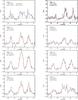 |
Fig. 2 N2H+ 1 → 0 spectra from the merged PdBI+MOPRA dataset (black lines) and the best fit parameters (red dashed lines, see Table 2). The positions seven hyperfine components (Caselli et al. 1995) are shown in the top-right panel. |
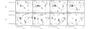 |
Fig. 3 Channel map of merged N2H+ emission. Contours are plotted at −50 (dotted), 50, 100, 150, and 200 mJy beam-1. The velocity channel is indicated in the upper-left of each panel in units of km s-1, and the blue plus signs indicate the centres of the main regions. The synthesised beam in shown in the lower-left corner of each panel. |
4. Results: Core environment traced by C18O
We use the emission from the 2 → 1 transition of C18O as a probe of the environment or “envelope” within
which the dense cores discussed above reside (cf. Walsh et
al. 2004; Kirk et al. 2007). The cores
themselves are of sufficiently high density that CO is preferentially frozen out onto dust
grains, eliminating the main destroyer of N2H+ (e.g. Bergin et al.
2002). In this region of G11, our 118
resolution C18O (2−1) maps show no significant small-scale peaks in common with the
continuum or N2H+, but rather a more extended morphology, similar to the
SPIRE 350 μm
emission (see Fig. 1a). As such, we treat the
C18O as a tracer of
the envelope.
By comparing the C18O emission to core properties probed by N2H+ discussed above, we will measure
the relationship between the cores and their environment. We show the C18O (2−1) spectra extracted at the positions of the
three regions (averaging over 118
diameter circle) in Fig. 4. A single Gaussian component
can satisfactorily fit the C18O (2−1) line, the parameters of which are given in Table 3. Region 3 exhibits a hint of wing emission, which may
be consistent with an outflow from an internal source. We experimented with two-component
fits in an attempt to address the slight blue asymmetry, but this did not improve the fit
quality (cf. Jiménez-Serra et al. 2014).
The velocity centroids of the C18O (2−1) are consistently between 29.4 and 29.7 km s-1, consistent within uncertainties with the centroids in the N2H+ spectra. The C18O (2−1) line is broadest in region 1, where two velocity components are detected in N2H+ (1−0), but no counterpart to the 32 km s-1 component seen in core 1a is seen in C18O4. In summary, the C18O (2−1) emission is fairly uniform over this region, with a mean Tmb = 0.93 K, vlsr = 29.52 km s-1 and Δv = 1.90 km s-1 (FWHM).
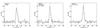 |
Fig. 4 Solid lines show spectra of C18O (2−1) (green) from the IRAM 30-m telescope averaged over the 12′′ regions (see Table 1), and the dashed green lines show the best single component Gaussian fits to the data. The fit parameters are summarised in Table 3. The red vertical line indicates the velocity centroid from the fits to the PdBI+MOPRA N2H+ (1−0) data. |
5. Discussion
5.1. Virial analysis
The virial mass (Mvir) provides an estimate of how gravitationally bound a core is: a core which exceeds its virial mass by a factor of 2 or more is considered self-gravitating. We assume an underlying density profile of ρ ∝ R-1.8, where R is the core radius, for the cores based on the median value found by Shirley et al. (2002) in their study of Class 0 protostars. Following MacLaren et al. (1988), we calculate the virial mass for cores with the assumed density profile, the expression for which is Mvir = 147 R (Δv)2, where R is the core radius in parsecs evaluated in the combined N2H+ map, and Δv is the N2H+ linewidth (FWHM) in km s-1. The derived values, which are listed in Table 2, range from 6 M⊙ in region 1 to 44 M⊙ in region 3. These values would be elevated to 8 and 60 M⊙ if G11 is instead assumed to be at the extinction distance, 4.7 kpc.
We compare the submillimetre mass (M350 μm, Table 1) in the main regions to the virial masses computed at the main (“a”) peaks in the N2H+ combined PdBI+MOPRA maps. We find a virial parameter (αvir = Mvir/M350 μm) of 1.1 and 2.5 (1.5 and 3.5 for 4.7 kpc distance) for regions 2 and 3, respectively, values which are close to the “critical” boundary of ~2 below which objects are considered unstable to collapse. As there are two velocity components in region 1, we estimate virial masses for each: 6.5 M⊙ (29.7 km s-1 component) and 29.5 M⊙ (32.0 km s-1 component). Because the mass is summed in that line of sight, it is not possible to say how much mass corresponds to each velocity component. Either way, M350 μm of region 1 is within a factor of ~2 of the virial mass. These α values are typical of what is observed in high-mass regions throughout the literature (Kauffmann et al. 2013).
As was pointed out by Ballesteros-Paredes (2006) in the context of a turbulent ISM, we caution the reader that considering the cores in isolation is a flawed approach in determining core stability. Indeed the cores may represent the sites of local collapse favoured in such an environment. If we consider the boundedness of the entire region of radius R~ 0.8 pc (approximating as a sphere), which exhibits an average linewidth of 1.9 km s-1 (σ = 0.81 km s-1) in C18O, and contains ~700 M⊙ from dust continuum emission (Henning et al. 2010), the virial mass, given in this case by Mvir = 126 R (Δv)2 (assuming ρ ∝ R-2) is ~360 M⊙, resulting in a virial parameter ~0.5. From this, we would conclude that this region is likely undergoing collapse from large scales, similar to global trends seen by Ragan et al. (2012a). However, we emphasise again that this simplistic analysis neglects any contribution from magnetic fields, uncertainties in the dust emissivity and other effects, any of which could contribute factors of a few to this analysis.
5.2. Fragmentation scale
We find the average nearest-neighbour separation between our sample of N2H+ cores (see Table 2) to be 0.18 pc. The cores have effective radii
(reff =
 ) ranging between 0.04 and 0.08 pc. Our
observations are not sensitive to the sub-structure of cores, but rather probe how the
large-scale IRDC filament sub-divides from clumps to cores (cf. Kainulainen et al. 2013; Wang et al.
2014). As G11 is a well-known filamentary IRDC, it is tempting to attribute the
nature of its fragmentation to the so-called “sausage instability”, which arises from the
collapse of an infinite isothermal cylinder (e.g. Chandrasekhar & Fermi 1953; Ostriker
1964). Kainulainen et al. (2013) showed
that on large length scales (l> 0.5 pc), a collapsing isothermal cylinder reasonably predicts the
structure separations, but on smaller scales such as those probed in this work, thermal
Jeans instability analysis appears a better match.
) ranging between 0.04 and 0.08 pc. Our
observations are not sensitive to the sub-structure of cores, but rather probe how the
large-scale IRDC filament sub-divides from clumps to cores (cf. Kainulainen et al. 2013; Wang et al.
2014). As G11 is a well-known filamentary IRDC, it is tempting to attribute the
nature of its fragmentation to the so-called “sausage instability”, which arises from the
collapse of an infinite isothermal cylinder (e.g. Chandrasekhar & Fermi 1953; Ostriker
1964). Kainulainen et al. (2013) showed
that on large length scales (l> 0.5 pc), a collapsing isothermal cylinder reasonably predicts the
structure separations, but on smaller scales such as those probed in this work, thermal
Jeans instability analysis appears a better match.
We first consider the region as a whole. The temperature in this region is ~12 K (Pillai et al. 2006a), the total mass is 700 M⊙ and the mean density is 104 cm-3 (Henning et al. 2010). The thermal Jeans fragmentation length5 applied at this scale is then ~0.2 pc, which agrees with the observed structure. The Jeans mass is 4 M⊙. The cores themselves have mean densities of 1−2 × 105 cm-3 and slightly higher temperatures (see Table 1, taking 20 K as a representative temperature), which predicts a fragment size of 0.09 pc, which agrees with the observed sizes, and mass of ~2 M⊙. We see that thermal Jeans fragmentation satisfactorily predicts the sizes and separations of the cores, similar to what has been observed in other young regions (e.g. Teixeira et al. 2006; Takahashi et al. 2013; Beuther et al. 2013). That M>MJeans indicates that, in the absence of other means of support, we expect the cores to fragment further beyond the resolution of our observations.
5.3. Core evolution signatures
Our continuum studies of this region have provided us with a means with which to assess the evolutionary stage of the cores, i.e. regions 1, 2 and 3. Table 1 lists the bolometric temperature (Tbol, Myers & Ladd 1993), which was determined by integrating the SED over all available data and deriving the characteristic temperature. This method has proven especially useful in analysing new protostellar populations discovered in Herschel data (e.g. Stutz et al. 2013; Ragan et al. 2012b). Simply, as a core evolves, its Tbol increases. Due to the small sample size under discussion here, we merely use Tbol as a proxy for relative evolutionary stage and do not speculate further whether the trends seen in the line emission hold universally. Strictly speaking, all cores fall below the fiducial Tbol = 70 K threshold proposed by André et al. (1993), qualifying all sources as Class 0 cores, but as was demonstrated in Ragan et al. (2013) and Stutz et al. (2013), Tbol faithfully follows the evolution within this phase, such that more evolved cores have higher values of Tbol.
We consider the kinematic properties of the cores in the context of their evolutionary stage as probed by the infrared characteristics. If we assume that continuum regions 1, 2 and 3 (Table 1) correspond most closely with emission from N2H+ cores 1a, 2a and 3a (Table 2), then the linewidth of N2H+ clearly increases with advancing evolution, i.e. increasing Tbol. The C18O linewidth is larger in region 3 than in region 2, but broadest in starless region 1. The latter may be due to unresolved multiple components (though not at the same separation in velocity as N2H+ core 1a and 1a′, see Sect. 5.4), but as it stands no correlation is apparent in C18O. Inspection of 13CO (2−1) spectra at the same positions (not shown) exhibit identical linewidths over the entire region of ~4 km s-1.
5.4. IRDC core kinematics
There is general agreement between observations and cluster formation theories that star-forming cores are found at over-densities in turbulent molecular clouds, however the dynamical aspect of this condition is still debated. Growing observational evidence (e.g. Csengeri et al. 2011a; Ragan et al. 2012a; Peretto et al. 2013) has demonstrated that global infall and collapse are prevalent in the early stages of (high-mass) star formation, challenging the assumptions of quasi-static initial conditions (e.g. McKee & Tan 2003). However, if we are to adopt a more dynamical framework of the initial conditions of cluster formation, observational constraints of the kinematics on all scales are still lacking. In the following, we address several aspects of the dynamical environment.
5.4.1. Multiple velocity components in N2H+
In massive IRDCs, N2H+(1−0) emission is excited in extended regions, and when observed with a single dish telescope the derived linewidth is typically supersonic (cf. Tackenberg et al. 2014). However, when we restrict our view to scales below 0.1 pc (core scales), we often find that due to the exclusion of unrelated or extended material, the line widths are much narrower, enabling us to isolate multiple velocity components, the most striking example of which presents itself in core 1a (and 1a′). The separation of the line centroids is about 2.5 km s-1: much larger than separations observed in low-mass filaments (Hacar & Tafalla 2011; Hacar et al. 2013), slightly larger to what was seen (at the same spectral resolution) in 4 out of 17 cores observed in intermediate mass IRDC 19175 by Beuther & Henning (2009) and in IRDC filaments in G035.39-00.33 (Henshaw et al. 2014), but similar to velocity centroid separations observed in high-mass IRDCs (e.g. Csengeri et al. 2011b; Beuther et al. 2013; Peretto et al. 2013).
The ubiquity of multiple velocity components reported in the literature undeniably points to the importance of the dynamical picture in the early stages of cluster formation, on both large and small scales. In most of the studies mentioned above, the two velocity peaks in N2H+ are seen over parsec spatial scales, so it is possibly worth distinguishing these cases from instances in which the two components of dense gas tracers are restricted to individual cores such as Beuther & Henning (2009) and this work. Our target region in G11 does not exhibit multiple components separated by >1 km s-1 on large filamentary scales, but rather seems to be confined to core 1a and 1a′. Using simulations of isolated clouds, Smith et al. (2013) assert that such a signature in optically thin species, such as N2H+, can be simply explained by multiple density peaks along our sightline. However, our C18O (2−1) data shows that no counterpart to the second velocity component detected in N2H+, which would be expected if structure on the line of sight were the only cause. Another possibility for the origin of the second component in N2H+ is shocked emission arising from dense material gravitationally in-falling onto the young core 1a, possibly connected to the global collapse of the whole region. Further multi-tracer observations at ~0.1 pc resolution are required to determine the prevalence of this signature in dense, young objects.
5.4.2. Core motions
Core-to-core velocity dispersions in clouds may be a useful diagnostic in ascertaining whether turbulence is driven or decaying (Offner et al. 2008). In simulations with turbulent driving, prestellar cores displayed a higher core-to-core velocity dispersion than protostellar cores, and the reverse was true in simulations with decaying turbulence. Observational evidence for both scenarios exists: while Perseus (Kirk et al. 2007) agrees with driven turbulence, Ophiuchus (André et al. 2007) and NGC 2068 (Walker-Smith et al. 2013) agree better with the decaying turbulence scenario.
Our target region in the G11 IRDC offers an interesting case of intermediate and low-mass cores embedded in a large mass reservoir. Unfortunately, due to the limited region we were able to map, our sample size is too small to draw any strong conclusions. Nevertheless, assuming that this region in G11 is oriented roughly in the plane of the sky, the overall standard deviation of centroid velocities among the cores (see Table 2) is σ = 0.87 km s-1 (PdBI-only values) and 0.74 km s-1 (PdBI+MOPRA values). We find no significant variation between the line centroids of the two prototellar cores (1a and 2a, σ = 0.05 km s-1), and the core-to-core velocity dispersions for (apparently) prestellar/starless cores is higher, σ = 0.97 km s-1 (including core 1a′, 0.83 km s-1 for PdBI+MOPRA). Since σprestellar>σprotostellar, this region follows the trend seen for driven turbulence simulations, although this should be repeated with a much larger statistical sample of cores. Additionally, massive IRDC filaments are highly turbulent environments which were not the focus of the Offner et al. (2008) study, so we emphasise that this is not firm evidence against the decaying turbulence scenario.
We also compare the core motions with respect to the large scale gas reservoir traced by C18O. While the C18O is fairly uniform over this region, we note that the linewidth is most enhanced at the position of the two N2H+ velocity components (region 1). We do not, however, detect a corresponding velocity component to N2H+ core 1a with velocity ~32 km s-1; if a second C18O unresolved velocity component exists there, it is at a velocity closer to the systemic ~30 km s-1. Does this second N2H+ component indicate that the emitting core (1a′) is somehow decoupled from the larger mass reservoir? Or does it have a different origin altogether?
With the exception of core 1a′, the N2H+ core velocity centroids agree remarkably well with the velocity of C18O emission (their common reservoir). In the dynamical models posed by Bonnell et al. (2001a,b), Bonnell & Bate (2006), and Ayliffe et al. (2007), this coupling between cores and their reservoir indicates that the region is in an early stage at which cores can accrete effectively. This is similar to what has been observed in relatively low-mass environments (Walsh et al. 2004; Kirk et al. 2007, 2010; Walker-Smith et al. 2013), which generally find little or no offset between the velocity centroids of the high-density gas tracer and the tracer of the less dense mass reservoir, typically differing by less than the local sound speed.
6. Conclusions
We present new observations of a quiescent region in the IRDC G011.11-0.12. This region
contains three intermediate mass starless/protostellar cores which have previously been
characterised by Herschel and SABOCA. We have mapped the region in
N2H+ (1−0) with the Plateau de Bure Interferometer
along with the 3.2 mm continuum at 7.21′′×
2.97′′ (0.12 × 0.05 pc) resolution. We mapped the
C18O (2−1) transition with the IRAM 30-m telescope at
118
(~0.2 pc) resolution. We
summarise our results as follows:
-
We find the continuum emission traces the three primary, Herschel-identified cores. The continuum peaks also mark the maxima in integrated N2H+ emission. The N2H+ emission appears as a chain of cores with radii from 0.04 to 0.08 pc. The mean nearest neighbour separation is 0.18 pc. Both the core separations and their sizes are well-predicted by isothermal Jeans fragmentation, similar to other detailed studies at similar physical resolutions.
-
We find that the main continuum-identified regions have masses between factors 1.1 to 2.5 times less than the virial mass, placing them at the boundary between sub- and super-critical, but similar to the low-values of the virial parameter (αvir) cores observed in high-mass regions. However, we emphasise that the regions are located in a vast mass reservoir, which invalidates the basic assumptions of the virial theorem. Turning our attention to the stability of the whole region traced by single-dish observations, it is supercritical (αvir~ 0.5) and is thus likely undergoing large-scale gravitational collapse. We note that our analysis does not account for the contribution of magnetic fields or geometrical effects, which are needed for a more comprehensive understanding of the region’s stability.
-
Using the bolometric temperature (Tbol) as a proxy for relative evolutionary stage of the cores, we find the N2H+ linewidth increases with evolutionary stage, while the C18O shows a more modest increase, and 13CO shows none at all. This suggests that the kinematic feedback from embedded protostars is quite localised and/or at an early stage before prominent molecular outflows are evident.
-
The starless region 1, with M350 μm = 14 M⊙ and Tbol< 13 K, exhibits two clear velocity components in N2H+ in both the PdBI-only map and combined PdBI+MOPRA map, separated by 2.5 and 2.3 km s-1, respectively. Emission at the velocity of the second component is seen to extend south to another quiescent core (1b). Such two-component signatures do not appear in the N2H+ spectra of more evolved regions 2 and 3 and also do not have a counterpart in the C18O (2−1) spectrum. This observation amplifies the importance of not only the complex structure of young regions, but also the complex dynamics, such as global gravitational collapse or shocks, in understanding the initial phases of cluster formation.
-
The core velocities (from N2H+) match the characteristic velocity of the C18O, the probe of the common mass reservoir. The core-to-core dispersion is of the same order as the dispersion of the C18O (2−1) line. With the exception of core 1a′, the cores appear to be coupled to their common mass reservoir such that accretion can effectively proceed.
MOPRA is operated by the Australian Telescope National Facility (ATNF).
Assuming an extrapolated dust opacity (β = 1.7) from Col. 5 (n = 106 cm-3, thin ice mantles) of κ3 mm = 0.23 cm2 g-1Ossenkopf & Henning (1994), gas-to-dust mass ratio of 100, cold-component temperatures from Ragan et al. (2013).
We note that new observations of [CI] of this region show broadened line profile (Δv = 4.5 km s-1), corresponding to a broadening of C18O (2−1) line, 25′′ (0.4 pc) south of region 1 (Beuther et al. 2014).
In the context of non-uniform and supersonic environment of IRDCs, the Jeans length should be understood as an upper limit for equilibrium (Stahler & Palla 2005). The supersonic conditions in IRDCs, which may be driven by accretion from large scales (Klessen & Hennebelle 2010; Heitsch 2013), violate the assumptions inherent in basic Jeans analysis (Goodman et al. 1998). Other processes, such as turbulence, rotation or support from magnetic fields, could be influencing the observed structure as well.
Acknowledgments
We thank Jochen Tackenberg for kindly providing reduced MOPRA data, Anike Schmiedeke for supplying the Herschel EPoS team with reduced data, and Paul Clark for useful discussions. We thank the referee and editor for helpful comments which helped to improve the paper. S.E.R. acknowledges support from the Deutsche Forschungsgemeinschaft priority program 1573 (“Physics of the Interstellar Medium”). This research has made use of NASA Astrophysics Data System. This research made use of APLpy, an open-source plotting package for Python hosted at http://aplpy.github.com
References
- André, P., Ward-Thompson, D., & Barsony, M. 1993, ApJ, 406, 122 [NASA ADS] [CrossRef] [Google Scholar]
- André, P., Belloche, A., Motte, F., & Peretto, N. 2007, A&A, 472, 519 [NASA ADS] [CrossRef] [EDP Sciences] [Google Scholar]
- Ayliffe, B. A., Langdon, J. C., Cohl, H. S., & Bate, M. R. 2007, MNRAS, 374, 1198 [NASA ADS] [CrossRef] [Google Scholar]
- Ballesteros-Paredes, J. 2006, MNRAS, 372, 443 [NASA ADS] [CrossRef] [Google Scholar]
- Bergin, E. A., Alves, J., Huard, T., & Lada, C. J. 2002, ApJ, 570, L101 [NASA ADS] [CrossRef] [Google Scholar]
- Beuther, H., & Henning, T. 2009, A&A, 503, 859 [NASA ADS] [CrossRef] [EDP Sciences] [Google Scholar]
- Beuther, H., Linz, H., Tackenberg, J., et al. 2013, A&A, 553, A115 [NASA ADS] [CrossRef] [EDP Sciences] [Google Scholar]
- Beuther, H., Ragan, S. E., Ossenkopf, V., et al. 2014, A&A, 571, A53 [NASA ADS] [CrossRef] [EDP Sciences] [Google Scholar]
- Bonnell, I. A., & Bate, M. R. 2006, MNRAS, 624 [Google Scholar]
- Bonnell, I. A., Bate, M. R., Clarke, C. J., & Pringle, J. E. 2001a, MNRAS, 323, 785 [NASA ADS] [CrossRef] [Google Scholar]
- Bonnell, I. A., Clarke, C. J., Bate, M. R., & Pringle, J. E. 2001b, MNRAS, 324, 573 [NASA ADS] [CrossRef] [Google Scholar]
- Carey, S. J., Clark, F. O., Egan, M. P., et al. 1998, ApJ, 508, 721 [NASA ADS] [CrossRef] [Google Scholar]
- Carey, S. J., Feldman, P. A., Redman, R. O., et al. 2000, ApJ, 543, L157 [NASA ADS] [CrossRef] [Google Scholar]
- Caselli, P., Myers, P. C., & Thaddeus, P. 1995, ApJ, 455, L77 [NASA ADS] [CrossRef] [Google Scholar]
- Caselli, P., Benson, P. J., Myers, P. C., & Tafalla, M. 2002, ApJ, 572, 238 [NASA ADS] [CrossRef] [Google Scholar]
- Chandrasekhar, S., & Fermi, E. 1953, ApJ, 118, 116 [NASA ADS] [CrossRef] [MathSciNet] [Google Scholar]
- Csengeri, T., Bontemps, S., Schneider, N., Motte, F., & Dib, S. 2011a, A&A, 527, A135 [NASA ADS] [CrossRef] [EDP Sciences] [Google Scholar]
- Csengeri, T., Bontemps, S., Schneider, N., et al. 2011b, ApJ, 740, L5 [NASA ADS] [CrossRef] [Google Scholar]
- Egan, M. P., Shipman, R. F., Price, S. D., et al. 1998, ApJ, 494, L199 [NASA ADS] [CrossRef] [Google Scholar]
- Gerner, T., Beuther, H., Semenov, D., et al. 2014, A&A, 563, A97 [NASA ADS] [CrossRef] [EDP Sciences] [Google Scholar]
- Gómez, L., Wyrowski, F., Pillai, T., Leurini, S., & Menten, K. M. 2011, A&A, 529, A161 [NASA ADS] [CrossRef] [EDP Sciences] [Google Scholar]
- Goodman, A. A., Barranco, J. A., Wilner, D. J., & Heyer, M. H. 1998, ApJ, 504, 223 [NASA ADS] [CrossRef] [Google Scholar]
- Griffin, M. J., Abergel, A., Abreu, A., et al. 2010, A&A, 518, L3 [Google Scholar]
- Hacar, A., & Tafalla, M. 2011, A&A, 533, A34 [NASA ADS] [CrossRef] [EDP Sciences] [Google Scholar]
- Hacar, A., Tafalla, M., Kauffmann, J., & Kovács, A. 2013, A&A, 554, A55 [NASA ADS] [CrossRef] [EDP Sciences] [Google Scholar]
- Heitsch, F. 2013, ApJ, 769, 115 [NASA ADS] [CrossRef] [Google Scholar]
- Henning, T., Linz, H., Krause, O., et al. 2010, A&A, 518, L95 [NASA ADS] [CrossRef] [EDP Sciences] [Google Scholar]
- Henshaw, J. D., Caselli, P., Fontani, F., Jiménez-Serra, I., & Tan, J. C. 2014, MNRAS, 440, 2860 [NASA ADS] [CrossRef] [Google Scholar]
- Jiménez-Serra, I., Caselli, P., Fontani, F., et al. 2014, MNRAS, 439, 1996 [NASA ADS] [CrossRef] [Google Scholar]
- Johnstone, D., Fiege, J. D., Redman, R. O., Feldman, P. A., & Carey, S. J. 2003, ApJ, 588, L37 [NASA ADS] [CrossRef] [Google Scholar]
- Kainulainen, J., Alves, J., Beuther, H., Henning, T., & Schuller, F. 2011, A&A, 536, A48 [NASA ADS] [CrossRef] [EDP Sciences] [Google Scholar]
- Kainulainen, J., Ragan, S. E., Henning, T., & Stutz, A. 2013, A&A, 557, A120 [NASA ADS] [CrossRef] [EDP Sciences] [Google Scholar]
- Kauffmann, J., Pillai, T., & Goldsmith, P. F. 2013, ApJ, 779, 185 [NASA ADS] [CrossRef] [Google Scholar]
- Kirk, H., Johnstone, D., & Tafalla, M. 2007, ApJ, 668, 1042 [NASA ADS] [CrossRef] [Google Scholar]
- Kirk, H., Pineda, J. E., Johnstone, D., & Goodman, A. 2010, ApJ, 723, 457 [NASA ADS] [CrossRef] [Google Scholar]
- Klessen, R. S., & Hennebelle, P. 2010, A&A, 520, A17 [NASA ADS] [CrossRef] [EDP Sciences] [Google Scholar]
- MacLaren, I., Richardson, K. M., & Wolfendale, A. W. 1988, ApJ, 333, 821 [NASA ADS] [CrossRef] [Google Scholar]
- Marshall, D. J., Joncas, G., & Jones, A. P. 2009, ApJ, 706, 727 [NASA ADS] [CrossRef] [Google Scholar]
- McKee, C. F., & Tan, J. C. 2003, ApJ, 585, 850 [NASA ADS] [CrossRef] [MathSciNet] [Google Scholar]
- Miettinen, O., & Offner, S. S. R. 2013, A&A, 555, A41 [NASA ADS] [CrossRef] [EDP Sciences] [Google Scholar]
- Myers, P. C., & Ladd, E. F. 1993, ApJ, 413, L47 [NASA ADS] [CrossRef] [Google Scholar]
- Offner, S. S. R., Krumholz, M. R., Klein, R. I., & McKee, C. F. 2008, AJ, 136, 404 [NASA ADS] [CrossRef] [Google Scholar]
- Ossenkopf, V., & Henning, T. 1994, A&A, 291, 943 [NASA ADS] [Google Scholar]
- Ostriker, J. 1964, ApJ, 140, 1056 [NASA ADS] [CrossRef] [MathSciNet] [Google Scholar]
- Perault, M., Omont, A., Simon, G., et al. 1996, A&A, 315, L165 [NASA ADS] [Google Scholar]
- Peretto, N., Fuller, G. A., Duarte-Cabral, A., et al. 2013, A&A, 555, A112 [NASA ADS] [CrossRef] [EDP Sciences] [Google Scholar]
- Pilbratt, G. L., Riedinger, J. R., Passvogel, T., et al. 2010, A&A, 518, L1 [CrossRef] [EDP Sciences] [Google Scholar]
- Pillai, T., Wyrowski, F., Carey, S. J., & Menten, K. M. 2006a, A&A, 450, 569 [NASA ADS] [CrossRef] [EDP Sciences] [Google Scholar]
- Pillai, T., Wyrowski, F., Menten, K. M., & Krügel, E. 2006b, A&A, 447, 929 [NASA ADS] [CrossRef] [EDP Sciences] [Google Scholar]
- Poglitsch, A., Waelkens, C., Geis, N., et al. 2010, A&A, 518, L2 [NASA ADS] [CrossRef] [EDP Sciences] [Google Scholar]
- Ragan, S. E., Bergin, E. A., Plume, R., et al. 2006, ApJS, 166, 567 [NASA ADS] [CrossRef] [Google Scholar]
- Ragan, S. E., Heitsch, F., Bergin, E. A., & Wilner, D. 2012a, ApJ, 746, 174 [NASA ADS] [CrossRef] [Google Scholar]
- Ragan, S. E., Henning, T., Krause, O., et al. 2012b, A&A, 547, A49 [NASA ADS] [CrossRef] [EDP Sciences] [Google Scholar]
- Ragan, S. E., Henning, T., & Beuther, H. 2013, A&A, 559, A79 [NASA ADS] [CrossRef] [EDP Sciences] [Google Scholar]
- Reid, M. J., Menten, K. M., Zheng, X. W., et al. 2009, ApJ, 700, 137 [NASA ADS] [CrossRef] [Google Scholar]
- Sanhueza, P., Jackson, J. M., Foster, J. B., et al. 2013, ApJ, 773, 123 [NASA ADS] [CrossRef] [Google Scholar]
- Shirley, Y. L., Evans, N. J., & Rawlings, J. M. C. 2002, ApJ, 575, 337 [NASA ADS] [CrossRef] [Google Scholar]
- Smith, R. J., Shetty, R., Beuther, H., Klessen, R. S., & Bonnell, I. A. 2013, ApJ, 771, 24 [NASA ADS] [CrossRef] [Google Scholar]
- Stahler, S. W., & Palla, F. 2005, The Formation of Stars (Wiley-VCH) [Google Scholar]
- Stutz, A. M., Tobin, J. J., Stanke, T., et al. 2013, ApJ, 767, 36 [NASA ADS] [CrossRef] [Google Scholar]
- Tackenberg, J., Beuther, H., Henning, T., et al. 2014, A&A, 565, A101 [NASA ADS] [CrossRef] [EDP Sciences] [Google Scholar]
- Tafalla, M., Myers, P. C., Caselli, P., & Walmsley, C. M. 2004, A&A, 416, 191 [NASA ADS] [CrossRef] [EDP Sciences] [Google Scholar]
- Takahashi, S., Ho, P. T. P., Teixeira, P. S., Zapata, L. A., & Su, Y.-N. 2013, ApJ, 763, 57 [NASA ADS] [CrossRef] [Google Scholar]
- Teixeira, P. S., Lada, C. J., Young, E. T., et al. 2006, ApJ, 636, L45 [NASA ADS] [CrossRef] [Google Scholar]
- Tobin, J. J., Bergin, E. A., Hartmann, L., et al. 2013, ApJ, 765, 18 [NASA ADS] [CrossRef] [Google Scholar]
- Vasyunina, T., Linz, H., Henning, T., et al. 2011, A&A, 527, A88 [NASA ADS] [CrossRef] [EDP Sciences] [Google Scholar]
- Walker-Smith, S. L., Richer, J. S., Buckle, J. V., et al. 2013, MNRAS, 429, 3252 [NASA ADS] [CrossRef] [Google Scholar]
- Walsh, A. J., Myers, P. C., & Burton, M. G. 2004, ApJ, 614, 194 [NASA ADS] [CrossRef] [Google Scholar]
- Wang, K., Zhang, Q., Testi, L., et al. 2014, MNRAS, 439, 3275 [NASA ADS] [CrossRef] [Google Scholar]
All Tables
All Figures
|
Fig. 1 a) Full G11 filament seen at 70 μm with Herschel/PACS with SPIRE 350 μm contours over-plotted from 9 Jy beam-1 increasing in steps of 3 Jy beam-1 (adapted from Henning et al. 2010). The SPIRE 350 μm beam (FWHM) is shown in the lower-left corner. The white rectangle marks the area shown in the rest of the panels. b) MIPS 24 μm image with 3.2 mm continuum contours from a PdBI-only map. The contour levels are from 0.2 to 0.12 mJy beam-1 in steps of 0.2 mJy beam-1. The synthesised beam is shown in the lower-left corner. c) APEX-SABOCA 350 μm continuum contours (Ragan et al. 2013) at 0.81, 1.08, 1.35 Jy beam-1 plotted over the PACS 100 μm image. The SABOCA 350 μm beam (FWHM) is shown in the lower left. d) Integrated intensity of N2H+ (1−0) from the PdBI-only map. e) Integrated intensity of the combined PdBI+MOPRA map. Both d) and e) are integrated from 29 to 33 km s-1, and the units of the colourscale are Jy beam-1km s-1. The + signs indicate the positions of the main continuum cores identified in panel b) and Table 1. |
| In the text | |
|
Fig. 2 N2H+ 1 → 0 spectra from the merged PdBI+MOPRA dataset (black lines) and the best fit parameters (red dashed lines, see Table 2). The positions seven hyperfine components (Caselli et al. 1995) are shown in the top-right panel. |
| In the text | |
|
Fig. 3 Channel map of merged N2H+ emission. Contours are plotted at −50 (dotted), 50, 100, 150, and 200 mJy beam-1. The velocity channel is indicated in the upper-left of each panel in units of km s-1, and the blue plus signs indicate the centres of the main regions. The synthesised beam in shown in the lower-left corner of each panel. |
| In the text | |
|
Fig. 4 Solid lines show spectra of C18O (2−1) (green) from the IRAM 30-m telescope averaged over the 12′′ regions (see Table 1), and the dashed green lines show the best single component Gaussian fits to the data. The fit parameters are summarised in Table 3. The red vertical line indicates the velocity centroid from the fits to the PdBI+MOPRA N2H+ (1−0) data. |
| In the text | |
Current usage metrics show cumulative count of Article Views (full-text article views including HTML views, PDF and ePub downloads, according to the available data) and Abstracts Views on Vision4Press platform.
Data correspond to usage on the plateform after 2015. The current usage metrics is available 48-96 hours after online publication and is updated daily on week days.
Initial download of the metrics may take a while.