Properties and nature of Be stars

P. Harmanec; P. Koubský; J. A. Nemravová; F. Royer; D. Briot; P. North; P. Lampens; Y. Frémat; S. Yang; H. Božić; L. Kotková; P. Škoda; M. Šlechta; D. Korčáková; M. Wolf; P. Zasche

doi:10.1051/0004-6361/201424640

Home

All issues

Volume 573 (January 2015)

A&A, 573 (2015) A107

Full HTML

Free Access

Issue		A&A Volume 573, January 2015


Article Number		A107
Number of page(s)		17
Section		Stellar structure and evolution
DOI		https://doi.org/10.1051/0004-6361/201424640
Published online		06 January 2015

A&A 573, A107 (2015)

30. Reliable physical properties of a semi-detached B9.5e+G8III binary BR CMi = HD 61273 compared to those of other well studied semi-detached emission-line binaries^⋆,^⋆⋆

P. Harmanec¹, P. Koubský², J. A. Nemravová¹, F. Royer³, D. Briot³, P. North⁴, P. Lampens⁵, Y. Frémat⁵, S. Yang⁶, H. Božić⁷, L. Kotková², P. Škoda², M. Šlechta², D. Korčáková¹, M. Wolf¹ and P. Zasche¹

¹ Astronomical Institute of the Charles University, Faculty of Mathematics and Physics, V Holešovičkách 2, 180 00 Praha 8 – Troja, Czech Republic
e-mail: Petr.Harmanec@mff.cuni.cz
² Astronomical Institute, Academy of Sciences of the Czech Republic, 251 65 Ondřejov, Czech Republic
³ GEPI/CNRS UMR 8111, Observatoire de Paris, Université Paris Denis Diderot, 5 place Jules Janssen, 92910 Meudon, France
⁴ Laboratoire d’astrophysique, École Polytechnique Fédérale de Lausanne (EPFL), Observatoire de Sauverny, 1290 Versoix, Switzerland
⁵ Royal Observatory of Belgium, Ringlaan 3, 1180 Brussel, Belgium
⁶ Physics & Astronomy Department, University of Victoria, PO Box 3055 STN CSC, Victoria, BC, V8W 3P6, Canada
⁷ Hvar Observatory, Faculty of Geodesy, University of Zagreb, Kačićeva 26, 10000 Zagreb, Croatia

Received: 20 July 2014
Accepted: 25 October 2014

Abstract

Reliable determination of the basic physical properties of hot emission-line binaries with Roche-lobe filling secondaries is important for developing the theory of mass exchange in binaries. It is a very hard task, however, which is complicated by the presence of circumstellar matter in these systems. So far, only a small number of systems with accurate values of component masses, radii, and other properties are known. Here, we report the first detailed study of a new representative of this class of binaries, BR CMi, based on the analysis of radial velocities and multichannel photometry from several observatories, and compare its physical properties with those for other well-studied systems. BR CMi is an ellipsoidal variable seen under an intermediate orbital inclination of ∼ 51^°, and it has an orbital period of 12 $.^{d}$ $\hbox{$.\!\!^{\rm d}$}$ 919059(15) and a circular orbit. We used the disentangled component spectra to estimate the effective temperatures 9500(200) K and 4655(50) K by comparing them with model spectra. They correspond to spectral types B9.5e and G8III. We also used the disentangled spectra of both binary components as templates for the 2D cross-correlation to obtain accurate radial velocities and a reliable orbital solution. Some evidence of a secular period increase at a rate of (1.1 ± 0.5) s per year was found. This, together with a very low mass ratio of 0.06 and a normal mass and radius of the mass gaining component, indicates that BR CMi is in a slow phase of the mass exchange after the mass-ratio reversal. It thus belongs to a still poorly populated subgroup of Be stars for which the origin of Balmer emission lines is safely explained as a consequence of mass transfer between the binary components.

Key words: binaries: close / binaries: spectroscopic / stars: emission-line, Be / stars: individual: BR CMi (HD 61273) / stars: fundamental parameters

^⋆

Based on new spectroscopic and photometric observations from the following instruments: Elodie spectrograph of the Haute Provence Observatory, France; CCD coudé spectrograph of the Astronomical Institute AS ČR at Ondřejov, Czech Republic; CCD coudé spectrograph of the Dominion Astrophysical Observatory, Canada; HERMES spectrograph attached to the Mercator Telescope, operated on the island of La Palma by the Flemish Community, at the Spanish Observatorio del Roque de los Muchachos of the Instituto de Astrofísica de Canarias; 7-C photometer attached to the Mercator Telescope, La Palma, UBV photometers at Hvar and Sutherland, and H_p photometry from the ESA Hipparcos mission.

^⋆⋆

Appendices are available in electronic form at http://www.aanda.org

© ESO, 2015

1. Introduction

In spite of the concentrated effort of several generations of astronomers, the very nature of the Be phenomenon – the presence of the Balmer emission lines in the spectra of some stars of spectral type B and their temporal variability on several time scales – is still not well understood. The competing hypotheses include (i) outflow of material from stellar photospheres, facilitated either by rotational instability at the stellar equator, by stellar wind, or by non-radial pulsations (or a combination of these effects); and (ii) several versions of mechanisms facilitated by the duplicity of the objects in question. It is true that the number of known binaries among Be stars is steadily increasing, but clear evidence that the Balmer emission is a consequence of the binary nature of the Be star in question exists only for Be stars, which have a mass-losing secondary that fills its Roche lobe. The number of known systems of this type with reliably determined physical properties is still rather small, and finding new representatives of this subgroup of Be binaries is desirable, not only for understanding Be stars but also from the point of view of the still developing theory of mass transfer in semi-detached binaries (see, e.g., the recent studies by Deschamps et al. 2013 or Davis et al. 2014). This paper deals with one such system.

Table 1

Journal of RV data sets.

BR CMi (HD 61273, BD+08^◦1831, SAO 115739, IRAS 07361+0804, HIP 37232) has not been studied much. Its light variability was discovered by Stetson (1991) from his uvbyβ observations, but his individual observations have never been published. The variability was rediscovered by Perryman & ESA (1997) with the Hipparcos satellite, and a period of 6 $.^{d}$ $\hbox{$.\!\!^{\rm d}$}$ 46 was reported by them. Kazarovets et al. (1999) classified it as a α² CVn variable and assigned it a variable-star name BR CMi. Paunzen et al. (2001) included this star into their list of λ Boo candidates but conclude that it is a normal star of spectral type A6V. In preliminary studies, Briot & Royer (2009) and Royer et al. (2007) announced that the object is actually a semi-detached Be dwarf and K0 giant binary and an ellipsoidal variable with an orbital period of 12 $.^{d}$ $\hbox{$.\!\!^{\rm d}$}$ 9190 and a mass ratio M_K/M_B = 0.14. Hereafter, we call the Be star component 1 and the cool giant component 2. Renson & Manfroid (2009) included the object into their catalogue of Ap, HgMn, and Am stars, giving it a spectral class A2, while Dubath et al. (2011), who were testing automatic classification procedures, classified it as an ellipsoidal variable with a period of 12 $.^{d}$ $\hbox{$.\!\!^{\rm d}$}$ 913. We present the first detailed study of the system, based on a rich collection of spectral and photometric observations.

2. Observations and reductions

Spectroscopy: the star was observed at the Haute Provence (OHP), Ondřejov (OND), Dominion Astrophysical (DAO), and La Palma observatories. Table 1 gives a journal of all radial velocity (RV) observations. Details about the spectra reductions and RV measurements are given in Appendix A.

Photometry: we attempted to collect all available observations with known dates of observations. Basic information about all data sets can be found in Table 2 and the details on the photometric reductions and standardisation are in Appendix B. For convenience, we also publish all of our individual observations together with their HJDs there (in Tables B.3–B.6).

3. Finding reliable orbital elements

One always has to be cautious when analysing binaries with clear signatures of the presence of circumstellar matter in the system. The experience from other such systems shows that the RV curve of the Roche-lobe filling component is usually clean and defines its true orbit quite well, while the absorption lines of the mass-gaining component can be affected by the circumstellar matter, and their RV curves do not follow the true orbital motion (cf. Harmanec & Scholz 1993; Desmet et al. 2010).

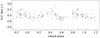Fig. 1

O−C residuals from the circular-orbit solution 2 for all RVs of component 2.

Table 2

Journal of available photometry for BR CMi.

To derive an improved ephemeris and an orbital solution for component 2, we used all its RVs measured in SPEFO (see Appendix A for details) and the program FOTEL (Hadrava 1990, 2004a). These solutions are summarised in Table 3. In solution 1, individual systemic (γ) velocities were derived for each spectrograph. Since our correction of the RV zero point via RV measurements of selected telluric lines clearly worked well (the γ velocities of all four instruments being nearly identical), we assumed that all RVs are on the same system and derived solution 2 with a joint systemic velocity. In this solution, we weighted the individual datasets 1−4 by weights inversely proportional to the squares of rms errors per one observation for each dataset from solution 1. As one can see in Fig. 1, the O−C residuals from the circular-orbit solution 2 define a low-amplitude double-wave phase curve. For that reason, we also tentatively derived an eccentric-orbit solution. It indeed led to an eccentricity of e = 0.0085 ± 0.0012, which is statistically significant according to the test by Lucy & Sweeney (1971). However, the corresponding longitude of periastron (referred to component 1) was ω = 93.3 ± 8.5 degrees, which is suspect. It is known that for tidally distorted components of binaries, the difference between the optical and mass centre of gravity leads inevitably to a deformation of the RV curve, which manifests itself by a false eccentricity with values of ω either 90^◦ or 270^◦ (Sterne 1941; Harmanec 2003; Eaton 2008). This is what also occurs for BR CMi and similar binaries, e.g. AU Mon (Desmet et al. 2010) or V393 Sco (Mennickent et al. 2012b).

Consequently, we adopted the circular-orbit solution 2 in Table 3 as a basis for a working new ephemeris (1) $T_{super . c .} = HJD 2 454 600.3806 (30) + 12 \overset{d}{.} 919046 (22) \cdot E .$ $\begin{equation} T_{\rm super.\,c.} = {\rm HJD}\,2\,454\,600.3806(30) + 12\fd919046(22) \cdot E.\label{efe1} \end{equation}$ (1)Next we measured and analysed the Hα profile. Selected Hα profiles stacked with increasing orbital phase are shown in Fig. 2. For binary Be stars with strong Hα emission, this is the best measure of the true orbital motion of the Be component – see Božić et al. (1995), Ruždjak et al. (2009) and Peters et al. (2013). This is not so for BR CMi, since its Hα emission rises to only 20% above the continuum level, and the measured RV curve of the Hα emission wings is poorly defined and has a phase shift with respect to expected orbital motion of component 1. In Fig. 2 one can also note that the width of both peaks of the double Hα emission varies systematically with the orbital phase, being largest shortly after both conjunctions. Figure 2 also shows the secular stability of the strength of Hα emission, with the observed changes mainly due to RV shifts of two absorption components, the stronger one associated with component 2 and a weaker one associated with material in the neighbourhood of component 1. It exhibits a RV curve, which is not in exact antiphase to that of component 2.

Table 3

Trial FOTEL orbital solutions based on RVs of component 2 measured in the program SPEFO.

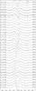Fig. 2

Selected Hα line profiles of BR CMi stacked with increasing orbital phase. Profiles are identified by cycle numbers and orbital phases with respect to ephemeris (1) and by RJDs = HJDs− 2 400 000.0. Symbols E, O, D, and H stand for Elodie, Ondřejov, DAO, and Hermes spectrographs.

In another attempt we used the program KOREL¹ developed by Hadrava (1995, 2004b) for spectra disentangling. Since the expected semi-amplitude of the orbital RV curve of component 1 is low, we decided to only analyse high-resolution Elodie and Hermes spectra from the blue spectral region between 4397 and 4608 Å. This region contains a number of He i and metallic lines but no Balmer line (to avoid contamination by the circumstellar matter). It turned out that because of relatively broad and not very numerous line profiles of component 1 and a low semi-amplitude of its RV curve, comparably good solutions could be obtained for a wide range of mass ratios. We note, however, that for the same reasons the disentangling of individual spectra is robust and can be trusted.

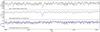Fig. 3

One observed Elodie spectrum and the disentangled spectra of components 1 and 2 in the wavelength interval 4397−4608 Å. The disentangled spectra were renormalised to their own continua and are compared to a model fit (see Sect. 4.1).

We then decided to try a cross-correlation in two dimensions, suggested (and realized as the program TODCOR) by Zucker & Mazeh (1994). In this technique, the individual observed spectra are compared to the two template spectra, which should closely correspond to the spectra of the two binary components, both in the spectral type and the projected rotational broadening. The RVs for both binary components are derived for each observed spectrum. A similar program to TODCOR was written by one of us (YF) under the name asTODCOR and has already been successfully applied to the case of AU Mon (Desmet et al. 2010). In practice, the Fourier transform of the observed and template spectra is computed via the FFT technique (Press et al. 1993). To meet the requirements of the FFT algorithm (see e.g. David et al. 2014), the spectra were rebinned to a smaller, constant, log λ bin size and apodised at both edges by means of a cosine-bell function. David & Verschueren (1995) showed that the combination of an even and uneven number of points correctly chosen around the CCF summit allows reducing the impact of discretisation on the measurement of its location, hence on the RV determinations. This approach was therefore also implemented in asTODCOR by combining the results of a parabola fit through three and four points.

It is usual practice to use suitable synthetic and properly rotationally broadened spectra as the templates. In this case, we used the spectra of both components disentangled by KOREL as the templates, adopting a preliminary estimated luminosity ratio L₂/L₁ = 0.25. The wavelength interval 4397−4608 Å was used (see Fig. 3), and we verified that the disentangled spectrum of component 1 had the same systemic velocity as component 2. The procedure worked remarkably well and returned well-defined RV curves for both binary components. This is seen in Fig. 4, which is the phase plot of these curves for ephemeris (1). We publish all individual SPEFO RVs for component 2 and asTODCOR RVs for both components, together with their HJDs in Tables A.2 and A.3.

Fig. 4

Top: orbital RV curve of both components of BR CMi based on RVs derived via 2D cross-correlation. Bottom: zoomed RV curve of component 1 from the upper panel showing how accurately the RVs were derived via the 2D cross-correlation.

In Table 4 we provide the circular-orbit solutions based on RVs resulting from 2D cross-correlation. Solution 3 is based on RVs of component 1 and solution 4 on RVs of component 2 alone. Their comparison shows that the epochs of superior conjunction of component 1 from both solutions agree with each other within the limits of their respective errors. They also agree with the epoch derived from a more numerous set of RVs from the red spectral region measured in SPEFO (see solution 2 of Table 3). Since the 2D cross-correlation puts no constraint on the derived RVs, this seems to prove that the RVs of component 1, found to be in exact antiphase to those of component 2, indeed reflect the true orbital motion of component 1. In addition, both solutions have identical RV zero points within its rms error of 0.1 km s^-1, confirming that using disentangled spectra has not introduced any biases. We therefore derived another solution 5, which is based on RVs for both binary components. It defines the M_1,2sin³i values and the mass ratio M₂/M₁ = 0.0593.

Table 4

FOTEL circular-orbit solutions individually for components 1 and 2 and for both stars together, based on RVs obtained via a 2D cross-correlation.

4. An estimate of basic physical elements of the binary components and the whole system

Since BR CMi is not an eclipsing but an ellipsoidal binary, its light curves can almost equally well be fitted for a wide range of possible orbital inclinations. For that reason, we proceeded in an iterative way, trying to describe all system properties in a mutually consistent way and taking all limitations we have at our disposal into account. In particular, we used the disentangled spectra of both binary components in several spectral regions to obtain good estimates of the effective temperatures of both stars via a comparison of disentangled and synthetic line profiles. These were then kept fixed in the combined light-curve and orbital solutions for a given inclination. Since the masses and radii thus obtained define log g quite accurately, we kept them fixed in the determination of T_eff.

4.1. Comparing the disentangled and interpolated model spectra

We used a program of J.A. Nemravová (see Nasseri et al. 2014) that interpolates in a precalculated grid of synthetic stellar spectra sampled in the effective temperature, gravitational acceleration, and metallicity. The synthetic spectra are compared to the disentangled ones for two or more components of a multiple system (normalised to the joint continuum of all bodies) and the initial parameters are optimised by minimisation of χ² until the best match is achieved.

Since the fractional luminosities within a considered spectral region are treated as independent of wavelength, we fitted the following six disentangled spectral bands separately: 4002−4039, 4142−4191, 4381−4435, 4446−4561, 4910−4960, and 8400−8880 Å. The interpolation was carried out in two different grids of spectra: AMBRE grid computed by de Laverny et al. (2012) was used for component 2, and the Pollux database computed by Palacios et al. (2010) was used for the hotter component 1.

It would not be wise to derive all physical parameters via free convergence in all considered spectral regions. Since the combined light and orbital solution can provide very tight values of log g and systemic velocity γ, we kept these values fixed in each superiteration between model spectra and combined solution. The infrared region 8400−8880 Å is the most appropriate region for the T_eff determination of component 2, since its fractional luminosity is much higher there (∼0.5 compared to less than 0.2 in the blue regions) and its spectrum is rich there.

Table 5

Average results of the final best fit of the interpolated grid of synthetic spectra to the observed ones in the six considered spectral regions.

Having the effective temperature of component 2 determined with an accuracy of ∼50 K, we kept it fixed in all five blue spectral regions, where the fractional luminosity of component 2 is low. The uncertainty of the fitted parameters has two components. The first is the statistical one connected with the photon noise and represents a minor contribution since the disentangled profiles have very high S/N. The second is influenced by the approach to the minimisation and can be estimated by repeating the fitting procedure and the need for (re)normalisation of the disentangled profiles². The former source of systematic error is not taken into account, because our program does not normalise the disentangled spectra. Therefore, we estimated the uncertainties of the optimised parameters as a mean of the best fit values obtained for each modelled spectral band, which should (at least to some degree) account for the need for (re)normalisation of the disentangled profile. The only exception is the uncertainty of the effective temperature of component 2, which was estimated via a simple Monte Carlo simulation. This is justified since the disentangled continua of component 2 were very close to a straight line in all regions. The results of the final minimisation averaged over all considered spectral regions are summarised in Table 5.

Table 6

Combined RV curve and light-curve solution.

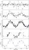Fig. 5

Comparison of the photometric observations (black points) with the PHOEBE model light curve corresponding to the χ² minimum for several photometric passbands (solid/blue line). The fits for the remaining passbands look similar. Phases from ephemeris 2 are used. Note the colour dependence of the amplitude of photometric changes on the wavelength.

4.2. A combined orbital and light-curve solution

We used the program PHOEBE (version 1.0 with a few custom passbands added; Prša & Zwitter 2005, 2006), all photometric data sets available to us, RVs of both components from the 2D cross-correlation and also RVs of component 2 measured in SPEFO because they give almost the same RV curve as the RVs from 2D cross-correlation but represent a much more numerous data set. For all Elodie and Hermes spectra, for which both sets of RVs of component 2 exist, we set their weights to 0.5 in both subsets. We assumed that component 2 fills the Roche lobe, fixed the mass ratio M₂/M₁ = 0.0593, which follows from the orbital solution for the cross-correlated RVs from spectra with high S/N (see solution 5 of Table 4).

An unsuccessful attempt to converge T_eff of component 1 was carried out. Changes of the T_eff did not lead to any improvement in the cost function value, and the program merely adjusted the radii of both components to adapt the model to the new temperature. We therefore decided to fix the effective temperatures of both components obtained from the fit of synthetic spectra to the disentangled ones. We adopted T_eff = 4655 K for component 2. The effective temperature of component 1 is rather uncertain. We therefore computed three sets of trial solutions for three different T_eff of the component 1 corresponding to the estimated 1σ bars given in Table 5: T_effϵ { 9343,9514,9685 } K. The solution that has the least χ² of all trial solutions is listed in Table 6. Error bars presented in Table 6 were estimated as the difference between the maximal (minimal) result of each parameter, which did not have the χ² greater than 1% of the χ² of the best solution, and the best solution. The bolometric albedos were estimated for the corresponding effective temperatures from Fig. 7 of Claret (2001) and the coefficients of gravity brightening from Fig. 7 of Claret (1998). Logarithmic limb-darkening coefficients were automatically interpolated after each iteration in PHOEBE from a pre-calculated grid of model atmospheres.

A test of the robustness of the final solution presented in Table 6 was carried out using the scripter environment of PHOEBE. We fitted the photometric observations and RVs from the 2D cross-correlation starting the convergence for 29 different initial orbital inclinations i ranging from 30 to 86 degrees. During each run, 30 iterations were computed, although the solution usually converged in less than ten iterations. The rotation parameter F (a ratio of spin to orbital revolution) of component 1 was not converged in PHOEBE , but it was optimised after each iteration using the new values of the component 1 radius and of the orbital inclination, while keeping the value of v sin i fixed from Table 5. A comparison of the optimal PHOEBE model light curves with the observed ones is in Fig. 5.

Table 7

List of some basic properties of well-observed semi-detached emission-line binaries.

The free convergence of the orbital period and epoch, now based not only on RVs but also on photometry, led to an improved linear ephemeris (2) $T_{super . c .} = HJD 2 454 600.38187 (42) + 12 \overset{d}{.} 9190594 (7) \cdot E .$ $\begin{equation} T_{\rm super.\,c.} = {\rm HJD}\,2\,454\,600.38187(42) + 12\fd9190594(7) \cdot E.\label{efe2} \end{equation}$ (2)To check on a secular constancy of the orbital period, we split the RVs and photometry into two subsets: HJD 2 448 705-53650 containing 460 data, and HJD 24 540 00-56295 containing 505 data. This particular choice ensured that both subsets contain a representative mixture of RVs and photometry. Local PHOEBE solutions for these two subsets led to the following linear ephemerides (3) and (4) 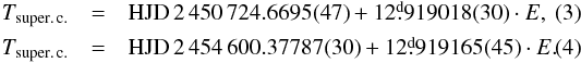$\begin{matrix} T_{super . c .} & = \\ T_{super . c .} & = \end{matrix}$ $\begin{eqnarray} T_{\rm super.\,c.} &=& {\rm HJD}\,2\,450\,724.6695(47) + 12\fd919018(30) \cdot E,\label{efe3}\\ T_{\rm super.\,c.} &=& {\rm HJD}\,2\,454\,600.37787(30) + 12\fd919165(45) \cdot E.\label{efe4} \end{eqnarray}$ They imply a secular increase in the orbital period for 3.8 × 10^-8 days per day or 1.2 s yr^-1. We therefore ran another PHOEBE solution on the complete data set, this time also allowing for the convergence of the secular period change. It provided a marginal support for the reality of a secular period increase of (3.5 ± 1.6) × 10^-8 d d^-1, the corresponding quadratic ephemeris (5) being 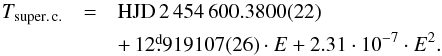$\begin{matrix} T_{super . c .} & = & HJD 2 454 600.3800 (22) \end{matrix}$ $\begin{eqnarray} T_{\rm super.\,c.} &=& {\rm HJD}\,2\,454\,600.3800(22)\nonumber\\ &&+\, 12\fd919107(26) \cdot E + 2.31\cdot10^{-7}\cdot E^2.\label{efe5} \end{eqnarray}$ (5)The original Hipparcos parallax (Perryman & ESA 1997) is 0.̋00670±0.̋00088. In van Leeuwen (2007b,a) an improved value of the Hipparcos parallax of BR CMi, 0.̋00579±0.̋00061 is given. These values imply a distance 132−172 pc for the original, and 156−193 pc for the improved value. A standard dereddening of UBV magnitudes of component 1 using the fractional luminosities of Table 6 gives V₀ = 7 $.^{m}$ $\hbox{$.\!\!^{\rm m}$}$ 08, ()₀ = −0 $.^{m}$ $\hbox{$.\!\!^{\rm m}$}$ 03, and ()₀ = −0 $.^{m}$ $\hbox{$.\!\!^{\rm m}$}$ 11 . These colours correspond to a normal B9.5 star, in agreement with the mean T_eff = 9685 K adopted as the best from the combined model fit of Table 6 for component 1. Consulting the tabulation of normal stellar masses and radii by Harmanec (1988), we find that the mass and radius of component 1, which follow from our solution, also correspond to a normal star of spectral type B9.5-A0 V. The range of M_bol = 1 $.^{m}$ $\hbox{$.\!\!^{\rm m}$}$ 01 − 1 $.^{m}$ $\hbox{$.\!\!^{\rm m}$}$ 18 for it implies M_V = 1 $.^{m}$ $\hbox{$.\!\!^{\rm m}$}$ 19 − 1 $.^{m}$ $\hbox{$.\!\!^{\rm m}$}$ 36 and a distance range of 139−151 pc. Our combined solution thus agrees with the observed distance of BR CMi. In passing, we also note that the effective temperature of component 2, based on the comparison of model and disentangled spectra, 4655 K, corresponds to spectral type G8 III according to a calibration by Popper (1980). The mass of component 2 is, however, much lower than the mass of a normal G8 giant, as usually found for the mass-losing stars in binaries.

5. BR CMi among other known emission-line semi-detached binaries

As already mentioned, the number of Be stars with known binary companions has been increasing steadily. However, many of them are single-line spectroscopic binaries and the nature of their companions is not known. There are some visual binaries among Be stars (Oudmaijer & Parr 2010). It is not clear how strong the mutual interaction between the components of such systems can be, although there is a suspicion of strong interaction during periastron passages in some systems with highly eccentric orbits like δ Sco (cf. Meilland et al. 2013, and references therein). Another distinct subgroup of Be binaries are systems with hot and compact secondaries, the prototype of such systems being ϕ Per (Gies et al. 1998; Božić et al. 1995). Only five such systems are known (see Koubský et al. 2012, 2014, and references therein). Finally, a subgroup of mass-exchanging semi-detached binaries exists in which the Be components are the mass-gaining components as predicted by the original binary hypothesis of the Be phenomenon (Kříž & Harmanec 1975; Harmanec & Kříž 1976).

There has also been recent progress in modelling the process of mass exchange in binaries (e.g. Siess et al. 2013; Deschamps et al. 2013; Davis et al. 2014) and obtaining reliable physical properties of mass-exchanging binaries is therefore essential for testing the predictions of new models. In Table 7, we collected a list of well-studied semi-detached emission-line binaries known to us and their published basic properties. We note that the spectral types quoted for mass gainers refer to the stellar bodies, not to the observed spectral classes affected by circumstellar matter. A zero secular change of the orbital period means that no significant change was detected in the available data.

The systems similar to those listed in Table 7 may not actually be very rare. We included only systems with reasonably safe evidence that one of the stars is filling its Roche lobe. The same might be true for the systems listed in Table 8, for which complete orbital and/or light-curve solutions and information on a secular orbital period change are still missing. Their detailed studies are very desirable. (Here, we have not included into consideration a number of short-periodic semi-detached binaries, for which transient Hα emission was reported in the astronomical literature.)

The list in Table 7 is too short to be statistically significant, but we use it to point out that there still might be a long way to a detailed comparison between observations and theory:

1.
One important observable is the equatorial rotational velocity of the gainer, but it is not often available even in new studies. For instance, Mennickent et al. (2012a) considered two models in their study of V393 Sco: spin-orbit synchonisation of the gainer and gainer with a break-up velocity. Available line profiles of the gainer show that its v sin i is somewhere in between these two cases, but this piece of information was not used. Our present study of BR CMi is probably one of the few where the synchronicity parameter F was changed after each iteration to correspond to the observed v sin i of the gainer.
2.
It is not obvious why some of these systems exhibit cyclic (if not periodic) light and colour changes on a time scale that is an order of magnitude longer than their respective orbital periods. For three of such variables, β Lyr, AU Mon, and V393 Sco, the presence of bipolar jets was considered. Similar jets were also considered for TT Hya, so a study of its long-term photometric behaviour would be of interest. Non-orbital light changes were also observed for UX Mon, but no clear periodicity was found. It is remarkable that UX Mon is a rare system at the early phase of the mass transfer before the mass ratio reversal. The differences in the orbital inclination also do not provide a clue. BR CMi and CX Dra are the only two non-eclipsing binaries in the considered sample, and while BR CMi seems to be secularly constant, CX Dra exhibits rather strong non-orbital long-term changes.
3.
Deschamps et al. (2013) tried to classify semi-detached binaries into three classes: I. systems before the mass ratio reversal; II. systems after the reversal but with still high rate of mass transfer; and III. systems in the quiescent final stages of mass transfer. We warn that the real situation may be even more complex and note that the secular period decrease would qualify SX Cas as a candidate for class I, while its observed masses clearly show that this is a system after mass reversal. Obviously, secular period changes may also be caused by other effects than the mass transfer between the components, for instance, by the presence of other bodies in the system. We can only conclude that the results of our study provide solid evidence that BR CMi is a system at the quiescent stages of mass transfer after the mass ratio reversal. It has the lowest mass ratio of all systems of Table 7.

Table 8

Other possibly semi-detached emission-line binaries.

Online material

Appendix A: Details of the spectral data reduction and measurements

The initial reduction of all Ondřejov and DAO spectra (bias subtraction, flat-fielding, creation of 1-D spectra, and wavelength calibration) was carried out in IRAF. For Elodie and Hermes spectra, dedicated reduction pipelines were used, combined with some IDL routines in the case of Elodie. See Baranne et al. (1996) and Raskin et al. (2011) for detailed descriptions of the Elodie and Hermes spectrographs. Rectification, removal of residual cosmics and flaws and RV measurements of all spectra were carried out with the program SPEFO (Horn et al. 1996; Škoda 1996), namely the latest version 2.63 developed by Mr. J. Krpata. SPEFO displays direct and flipped traces of the line profiles superimposed on the computer screen that the user can slide to achieve a precise overlapping of the parts of the profile of whose RV one wants to measure. Using a selection of stronger unblended lines of the cool component 2 (see Table A.1) covering the red spectral region (available for all spectra), we measured RVs of all of them to obtain a mean RV for all spectra. We also measured a selection of good telluric lines and used them for an additional fine correction of the RV zero point of

each spectrogram (Horn et al. 1996). Moreover, we measured the RVs of the steep wings of the Hα emission line and of the two absorption cores of Hα. We point out that although some broad and shallow lines of component 1 are seen in the spectra, their direct RV measurement is impossible because of numerous blends with the lines of component 2.

Table A.1

Spectral lines of component 2 and their air wavelengths used for the RV measurements in SPEFO.

Table A.2

Individual SPEFO RVs of component 2.

Table A.3

Individual asTODCOR RVs of both components.

Appendix B: Details on the photometric data reductions

Since we used photometry from various sources and photometric systems, both all-sky and differential, relative to several different comparison stars, we attempted to arrive at some homogenisation and standardisation. Special effort was made to derive improved all-sky values for the comparison stars used, employing carefully standardised UBV observations secured at Hvar over several decades of systematic observations. The adopted values are collected in Table B.1, together with the number of all-sky observations and the rms errors of one observation. They were added to the respective magnitude differences to obtain directly comparable standard UBV magnitudes for all stations. To illustrate the accuracy, with which various data sets were transformed to the standard system, we give (in Table B.2) mean differential UBV values for the check stars used. They were derived relatively to the Hvar values for the comparison stars HD 58187 and HD 61341.

Table B.1

Accurate Hvar and SAAO all-sky mean UBV values for all comparison stars used.

Table B.2

Mean UBV values for the check stars used at individual observing stations derived differentially relative to their respective comparison stars.

Below, we provide some details of the individual data sets and their reductions.

Station 01 – Hvar: these differential observations have been secured by HB and PZ relative to HD 58187 (the check star HD 59059 being observed as frequently as the variable) and carefully transformed to the standard UBV system via non-linear transformation formulæ using the HEC22 reduction program – see Harmanec et al. (1994) and Harmanec & Horn (1998) for the observational strategy and data reduction³. All observations were reduced with the latest HEC22 rel.17 program, which allows the time variation of linear extinction coefficients to be modelled in the course of observing nights.
Station 11 – South African Astronomical Observatory (SAAO): these differential UBV observations were obtained by PZ with the 0.50 m reflector relative to HD 61341 (SAO 115750 being used as the check star) and also transformed to the standard Johnson system with the help of HEC22.
Station 37 – La Palma: these all-sky seven-colour (7-C) observations were secured in the Geneva photometric system using the two-channel aperture photometer P7-2000 (Raskin et al. 2004) mounted on the 1.20 m Belgian Mercator reflector at the Observatorio de los Muchachos at La Palma.
Station 61 – Hipparcos: these all-sky observations were reduced to the standard V magnitude via the transformation formulæ derived by Harmanec (1998) to verify that no secular light changes in the system were observed. However, for the light-curve solution in PHOEBE, we consider the Hipparcos transmission curve for the H_p magnitude.
Station 93 – ASAS3 V photometry: we extracted these all-sky observations from the ASAS3 public archive (Pojmanski 2002), using the data for diaphragm 1, having on average the lowest rms errors. We omitted all observations of grade D and observations having rms errors larger than 0 $.^{m}$ $\hbox{$.\!\!^{\rm m}$}$ 04. We also omitted a strongly deviating observation at HJD 2 452 662.6863.

Table B.3

Individual Geneva 7-C observations.

Table B.4

Original Hipparcos H_p observations and their conversion to V band observations.

Table B.5

Individual ASAS-3 V band observations from diaphragm 1 without large errors.

Table B.6

Individual UBV band observations.

¹

The freely distributed version from Dec. 2004.

²

Since the disentangling in KOREL is carried out in Fourier space, it happens in almost every practical application that the resulting disentangled spectra after inverse Fourier transformation have slightly warped continua and need some re-normalisation.

³

The whole program suite with a detailed manual, examples of data, auxiliary data files, and results is available at http://astro.troja.mff.cuni.cz/ftp/hec/PHOT

Acknowledgments

This study uses spectral observations obtained with the HERMES spectrograph, which is supported by the Fund for Scientific Research of Flanders (FWO), Belgium, the Research Council of K.U. Leuven, Belgium, the Fonds National de la Recherche Scientifique (F.R.S.-FNRS), Belgium, the Royal Observatory of Belgium, the Observatoire de Genève, Switzerland and the Thüringer Landessternwarte Tautenburg, Germany, spectral observations with the Elodie spectrograph attached to 1.9 m reflector of Haute Provence Observatory, CCD spectrograph of the Ondřejov 2 m reflector, and CCD spectra from the spectrograph attached to the 1.22 m reflector of the Dominion Astrophysical Observatory. It also uses photometric observations made at the observatory of La Palma (Mercator), Hvar, and South African Astronomical Observatory (SAAO), and by the ESA Hipparcos satellite. We gratefully acknowledge the use of spectrograms of BR CMi from the public archives of the Elodie spectrograph of the Haute Provence Observatory and the use of the latest publicly available versions of the programs FOTEL and KOREL written by Dr. P. Hadrava. Our sincere thanks are also due to Dr. A. Prša, who provided us with a modified version of the program PHOEBE 1.0 and frequent consultations on its usage. We thank Drs. M. Ceniga, A. Kawka, J. Kubát, P. Mayer, P. Nemeth, M. Netolický, J. Polster, and V. Votruba, who obtained several Ondřejov spectra used in this study and to Dr. K. Uytterhoeven, who participated in photometric observations at La Palma. The comments of an anonymous referee helped to shorten the text and improve the presentation of the main results a great deal. This research was supported by the grants 205/06/0304, 205/08/H005, and P209/10/0715 of the Czech Science Foundation, by the grant 678212 of the Grant Agency of the Charles University in Prague, from the research project AV0Z10030501 of the Academy of Sciences of the Czech Republic, and from the Research Program MSM0021620860 Physical study of objects and processes in the solar system and in astrophysics of the Ministry of Education of the Czech Republic. The research of P.K. was supported from the ESA PECS grant 98058. H.B. acknowledges financial support from the Croatian Science Foundation under the project 6212 “Solar and Stellar Variability”. P.N. thanks the Swiss National Science Foundation for its support in acquiring photometric data in the Geneva 7-C system. We acknowledge the use of the electronic database from the CDS, Strasbourg, and the electronic bibliography maintained by the NASA/ADS system.

References

Ak, H.,Chadima, P.,Harmanec, P., et al. 2007, A&A, 463, 233 [NASA ADS] [CrossRef] [EDP Sciences] [Google Scholar]
Andersen, J.,Nordstrom, B.,Mayor, M., &Polidan, R. S. 1988, A&A, 207, 37 [NASA ADS] [Google Scholar]
Andersen, J.,Pavlovski, K., &Piirola, V. 1989, A&A, 215, 272 [NASA ADS] [Google Scholar]
Atwood-Stone, C.,Miller, B. P.,Richards, M. T.,Budaj, J., &Peters, G. J. 2012, ApJ, 760, 134 [NASA ADS] [CrossRef] [Google Scholar]
Baranne, A.,Queloz, D.,Mayor, M., et al. 1996, A&AS, 119, 373 [NASA ADS] [CrossRef] [EDP Sciences] [Google Scholar]
Bisikalo, D. V.,Harmanec, P.,Boyarchuk, A. A.,Kuznetsov, O. A., &Hadrava, P. 2000, A&A, 353, 1009 [NASA ADS] [Google Scholar]
Bopp, B. W.,Dempsey, R. C., &Parsons, S. B. 1991, PASP, 103, 444 [NASA ADS] [CrossRef] [Google Scholar]
Božić, H.,Harmanec, P.,Horn, J., et al. 1995, A&A, 304, 235 [NASA ADS] [Google Scholar]
Briot, D., & Royer, F. 2009, Be Star Newsletter No. 39, 15 [Google Scholar]
Burki, G., &Mayor, M. 1983, A&A, 124, 256 [NASA ADS] [Google Scholar]
Claret, A. 1998, A&AS, 131, 395 [NASA ADS] [CrossRef] [EDP Sciences] [Google Scholar]
Claret, A. 2001, MNRAS, 327, 989 [NASA ADS] [CrossRef] [Google Scholar]
Daems, K.,Waelkens, C., &Mayor, M. 1997, A&A, 317, 823 [NASA ADS] [Google Scholar]
David, M., &Verschueren, W. 1995, A&AS, 111, 183 [NASA ADS] [Google Scholar]
David, M.,Blomme, R.,Frémat, Y., et al. 2014, A&A, 562, A97 [NASA ADS] [CrossRef] [EDP Sciences] [Google Scholar]
Davis, P. J.,Siess, L., &Deschamps, R. 2014, A&A, 570, A25 [NASA ADS] [CrossRef] [EDP Sciences] [Google Scholar]
de Laverny, P.,Recio-Blanco, A.,Worley, C. C., &Plez, B. 2012, A&A, 544, A126 [NASA ADS] [CrossRef] [EDP Sciences] [Google Scholar]
Dempsey, R. C.,Bopp, B. W.,Parsons, S. B., &Fekel, F. C. 1990, PASP, 102, 312 [NASA ADS] [CrossRef] [Google Scholar]
Deschamps, R.,Siess, L.,Davis, P. J., &Jorissen, A. 2013, A&A, 557, A40 [NASA ADS] [CrossRef] [EDP Sciences] [Google Scholar]
Desmet, M.,Frémat, Y.,Baudin, F., et al. 2010, MNRAS, 401, 418 [NASA ADS] [CrossRef] [Google Scholar]
Djurašević, G.,Vince, I.,Khruzina, T. S., &Rovithis-Livaniou, E. 2009, MNRAS, 396, 1553 [NASA ADS] [CrossRef] [Google Scholar]
Dubath, P.,Rimoldini, L.,Süveges, M., et al. 2011, MNRAS, 414, 2602 [NASA ADS] [CrossRef] [Google Scholar]
Eaton, J. A. 2008, ApJ, 681, 562 [NASA ADS] [CrossRef] [Google Scholar]
Eggen, O. J. 1983, AJ, 88, 1676 [NASA ADS] [CrossRef] [Google Scholar]
Gies, D. R., Bagnuolo, Jr., W. G., Ferrara, E. C., et al. 1998, ApJ, 493, 440 [NASA ADS] [CrossRef] [Google Scholar]
Griffin, R. F.,Parsons, S. B.,Dempsey, R., &Bopp, B. W. 1990, PASP, 102, 535 [NASA ADS] [CrossRef] [Google Scholar]
Hadrava, P. 1990, Contr. Astron. Obs. Skalnaté Pleso, 20, 23 [Google Scholar]
Hadrava, P. 1995, A&AS, 114, 393 [NASA ADS] [Google Scholar]
Hadrava, P. 2004a, Publ. Astron. Inst. Acad. Sci. Czech Rep., 92, 1 [Google Scholar]
Hadrava, P. 2004b, Publ. Astron. Inst. Acad. Sci. Czech Rep., 92, 15 [Google Scholar]
Harmanec, P. 1988, Bull. Astron. Inst. Czechosl., 39, 329 [Google Scholar]
Harmanec, P. 1998, A&A, 335, 173 [NASA ADS] [Google Scholar]
Harmanec, P. 2002, Astron. Nachr., 323, 87 [NASA ADS] [CrossRef] [Google Scholar]
Harmanec, P. 2003, in Publ. Canakkale Onsekiz Mart Univ.: New Directions for Close Binary Studies: The Royal Road to the Stars, 3, 221 [Google Scholar]
Harmanec, P., &Horn, J. 1998, J. Astron. Data, 4, 5 [Google Scholar]
Harmanec, P., &Kříž, S. 1976, in Be and Shell Stars, ed. A. Slettebak, IAU Symp., 70, 385 [NASA ADS] [Google Scholar]
Harmanec, P., &Scholz, G. 1993, A&A, 279, 131 [NASA ADS] [Google Scholar]
Harmanec, P.,Horn, J., &Juza, K. 1994, A&AS, 104, 121 [NASA ADS] [Google Scholar]
Harmanec, P.,Morand, F.,Bonneau, D., et al. 1996, A&A, 312, 879 [NASA ADS] [Google Scholar]
Hill, G.,Harmanec, P.,Pavlovski, K., et al. 1997, A&A, 324, 965 [NASA ADS] [Google Scholar]
Horn, J.,Kubát, J.,Harmanec, P., et al. 1996, A&A, 309, 521 [NASA ADS] [Google Scholar]
Kazarovets, E. V.,Samus, N. N.,Durlevich, O. V., et al. 1999, IBVS, 4659, 1 [Google Scholar]
Koubský, P.,Harmanec, P.,Božić, H., et al. 1998, Hvar Observatory Bulletin, 22, 17 [NASA ADS] [Google Scholar]
Koubský, P.,Kotková, L.,Votruba, V.,Šlechta, M., &Dvořáková, Š. 2012, A&A, 545, A121 [NASA ADS] [CrossRef] [EDP Sciences] [Google Scholar]
Koubský, P.,Kotková, L.,Kraus, M., et al. 2014, A&A, 567, A57 [NASA ADS] [CrossRef] [EDP Sciences] [Google Scholar]
Kříž, S., &Harmanec, P. 1975, BAICz, 26, 65 [Google Scholar]
Linnell, A. P.,Harmanec, P.,Koubský, P., et al. 2006, A&A, 455, 1037 [NASA ADS] [CrossRef] [EDP Sciences] [Google Scholar]
Lucy, L. B., &Sweeney, M. A. 1971, AJ, 76, 544 [NASA ADS] [CrossRef] [Google Scholar]
Meilland, A.,Stee, P.,Spang, A., et al. 2013, A&A, 550, L5 [NASA ADS] [CrossRef] [EDP Sciences] [Google Scholar]
Mennickent, R. E.,Djurašević, G.,Kołaczkowski, Z., &Michalska, G. 2012a, MNRAS, 421, 862 [NASA ADS] [Google Scholar]
Mennickent, R. E.,Kołaczkowski, Z.,Djurašević, G., et al. 2012b, MNRAS, 427, 607 [NASA ADS] [CrossRef] [Google Scholar]
Miller, B.,Budaj, J.,Richards, M.,Koubský, P., &Peters, G. J. 2007, ApJ, 656, 1075 [NASA ADS] [CrossRef] [Google Scholar]
Moore, C. E. 1945, Contributions from the Princeton University Observatory, 20, D23 [Google Scholar]
Nasseri, A.,Chini, R.,Harmanec, P., et al. 2014, A&A, 568, A94 [NASA ADS] [CrossRef] [EDP Sciences] [Google Scholar]
Olson, E. C.,Henry, G. W., &Etzel, P. B. 2009, AJ, 138, 1435 [NASA ADS] [CrossRef] [Google Scholar]
Oudmaijer, R. D., &Parr, A. M. 2010, MNRAS, 405, 2439 [NASA ADS] [Google Scholar]
Palacios, A.,Gebran, M.,Josselin, E., et al. 2010, A&A, 516, A13 [NASA ADS] [CrossRef] [EDP Sciences] [Google Scholar]
Parsons, S. B., &Bopp, B. W. 1993, in American Astronomical Society Meeting Abstracts, BAAS, 25, 1376 [NASA ADS] [Google Scholar]
Parsons, S. B., Dempsey, R. C., & Bopp, B. W. 1988, in ESA SP, 281, 225 [Google Scholar]
Paunzen, E.,Duffee, B.,Heiter, U.,Kuschnig, R., &Weiss, W. W. 2001, A&A, 373, 625 [NASA ADS] [CrossRef] [EDP Sciences] [Google Scholar]
Perryman, M. A. C., & ESA 1997, The Hipparcos and Tycho catalogues, Astrometric and photometric star catalogues derived from the ESA Hipparcos Space Astrometry Mission (Noordwijk: ESA Publications Division) ESA SP Series 1200 [Google Scholar]
Peters, G. J.,Pewett, T. D.,Gies, D. R.,Touhami, Y. N., &Grundstrom, E. D. 2013, ApJ, 765, 2 [NASA ADS] [CrossRef] [Google Scholar]
Pojmanski, G. 2002, Acta Astron., 52, 397 [NASA ADS] [Google Scholar]
Popper, D. M. 1980, ARA&A, 18, 115 [NASA ADS] [CrossRef] [Google Scholar]
Press, W. H., Teukolsky, S. A., Vetterling, W. T., & Flannery, B. P. 1993, Numerical Recipes in FORTRAN; The Art of Scientific Computing, 2nd edn. (New York: Cambridge University Press) [Google Scholar]
Prša, A., &Zwitter, T. 2005, ApJ, 628, 426 [NASA ADS] [CrossRef] [Google Scholar]
Prša, A., & Zwitter, T. 2006, Ap&SS, 36 [Google Scholar]
Raskin, G., Burki, G., Burnet, M., et al. 2004, in Ground-based Instrumentation for Astronomy, eds. A. F. M. Moorwood, & M. Iye, SPIE Conf. Ser., 5492, 830 [Google Scholar]
Raskin, G., van Winckel, H.,Hensberge, H., et al. 2011, A&A, 526, A69 [NASA ADS] [CrossRef] [EDP Sciences] [Google Scholar]
Renson, P., &Manfroid, J. 2009, A&A, 498, 961 [NASA ADS] [CrossRef] [EDP Sciences] [Google Scholar]
Richards, M. T.,Koubský, P.,Šimon, V., et al. 2000, ApJ, 531, 1003 [NASA ADS] [CrossRef] [Google Scholar]
Royer, F., Briot, D., North, P., Burki, G., & Carrier, F. 2007, in IAU Symp. 240, eds. W. I. Hartkopf, E. F. Guinan, & P. Harmanec, 211 [Google Scholar]
Ruždjak, D.,Božić, H.,Harmanec, P., et al. 2009, A&A, 506, 1319 [NASA ADS] [CrossRef] [EDP Sciences] [Google Scholar]
Siess, L.,Izzard, R. G.,Davis, P. J., &Deschamps, R. 2013, A&A, 550, A100 [NASA ADS] [CrossRef] [EDP Sciences] [Google Scholar]
Škoda, P. 1996, in Astronomical Data Analysis Software and Systems V, ASP Conf. Ser., 101, 187 [NASA ADS] [Google Scholar]
Štefl, S.,Harmanec, P.,Horn, J., et al. 1990, BAICz, 41, 29 [NASA ADS] [Google Scholar]
Sterken, C.,Vogt, N., &Mennickent, R. 1994, A&A, 291, 473 [NASA ADS] [Google Scholar]
Sterne, T. E. 1941, PNAS, 27, 168 [NASA ADS] [CrossRef] [Google Scholar]
Stetson, P. B. 1991, AJ, 102, 589 [NASA ADS] [CrossRef] [Google Scholar]
Sudar, D.,Harmanec, P.,Lehmann, H., et al. 2011, A&A, 528, A146 [NASA ADS] [CrossRef] [EDP Sciences] [Google Scholar]
Szabados, L. 1990, A&A, 232, 381 [NASA ADS] [Google Scholar]
Tarasov, A. E.,Berdyugina, S. V., &Berdyugin, A. V. 1998, Astron. Lett., 24, 316 [NASA ADS] [Google Scholar]
van Leeuwen, F. 2007a, in Astrophys. Space Sci. Lib. 350 (Berlin: Springer) [Google Scholar]
van Leeuwen, F. 2007b, A&A, 474, 653 [NASA ADS] [CrossRef] [EDP Sciences] [Google Scholar]
Zucker, S., &Mazeh, T. 1994, ApJ, 420, 806 [NASA ADS] [CrossRef] [EDP Sciences] [MathSciNet] [Google Scholar]

All Tables

Table 1

Journal of RV data sets.

	Fig. 1 O−C residuals from the circular-orbit solution 2 for all RVs of component 2.
In the text

	Fig. 2 Selected Hα line profiles of BR CMi stacked with increasing orbital phase. Profiles are identified by cycle numbers and orbital phases with respect to ephemeris (1) and by RJDs = HJDs− 2 400 000.0. Symbols E, O, D, and H stand for Elodie, Ondřejov, DAO, and Hermes spectrographs.
In the text

	Fig. 3 One observed Elodie spectrum and the disentangled spectra of components 1 and 2 in the wavelength interval 4397−4608 Å. The disentangled spectra were renormalised to their own continua and are compared to a model fit (see Sect. 4.1).
In the text

	Fig. 4 Top: orbital RV curve of both components of BR CMi based on RVs derived via 2D cross-correlation. Bottom: zoomed RV curve of component 1 from the upper panel showing how accurately the RVs were derived via the 2D cross-correlation.
In the text

	Fig. 5 Comparison of the photometric observations (black points) with the PHOEBE model light curve corresponding to the χ² minimum for several photometric passbands (solid/blue line). The fits for the remaining passbands look similar. Phases from ephemeris 2 are used. Note the colour dependence of the amplitude of photometric changes on the wavelength.
In the text