| Issue |
A&A
Volume 573, January 2015
|
|
|---|---|---|
| Article Number | A12 | |
| Number of page(s) | 44 | |
| Section | Astrophysical processes | |
| DOI | https://doi.org/10.1051/0004-6361/201423983 | |
| Published online | 10 December 2014 | |
Late-time spectral line formation in Type IIb supernovae, with application to SN 1993J, SN 2008ax, and SN 2011dh⋆
1
Astrophysics Research Centre, School of Mathematics and Physics, Queen’s
University Belfast,
Belfast,
BT7 1NN,
UK
e-mail:
This email address is being protected from spambots. You need JavaScript enabled to view it.
2
The Oskar Klein Centre, Department of Astronomy, Stockholm
University, Albanova, 10691
Stockholm,
Sweden
3
Max-Planck-Institut für Astrophysik, Karl-Schwarzschild-Str. 1, 85741
Garching,
Germany
4
Kavli Institute for the Physics and Mathematics of the Universe
(WPI), Todai Institutes for Advanced Study, University of Tokyo,
5-1-5 Kashiwanoha, Kashiwa,
277-8583
Chiba,
Japan
5
ESO, Karl-Schwarzschild-Strasse 2, 85748
Garching,
Germany
Received: 11 April 2014
Accepted: 18 September 2014
Abstract
We investigate line formation processes in Type IIb supernovae (SNe) from 100 to 500 days post-explosion using spectral synthesis calculations. The modelling identifies the nuclear burning layers and physical mechanisms that produce the major emission lines, and the diagnostic potential of these. We compare the model calculations with data on the three best observed Type IIb SNe to-date − SN 1993J, SN 2008ax, and SN 2011dh. Oxygen nucleosynthesis depends sensitively on the main-sequence mass of the star and modelling of the [O I] λλ6300, 6364 lines constrains the progenitors of these three SNe to the MZAMS = 12−16 M⊙ range (ejected oxygen masses 0.3−0.9 M⊙), with SN 2011dh towards the lower end and SN 1993J towards the upper end of the range. The high ejecta masses from MZAMS ≳ 17 M⊙ progenitors give rise to brighter nebular phase emission lines than observed. Nucleosynthesis analysis thus supports a scenario of low-to-moderate mass progenitors for Type IIb SNe, and by implication an origin in binary systems. We demonstrate how oxygen and magnesium recombination lines may be combined to diagnose the magnesium mass in the SN ejecta. For SN 2011dh, a magnesium mass of 0.02−0.14 M⊙ is derived, which gives a Mg/O production ratio consistent with the solar value. Nitrogen left in the He envelope from CNO burning gives strong [N II] λλ6548, 6583 emission lines that dominate over Hα emission in our models. The hydrogen envelopes of Type IIb SNe are too small and dilute to produce any noticeable Hα emission or absorption after ~150 days, and nebular phase emission seen around 6550 Å is in many cases likely caused by [N II] λλ6548, 6583. Finally, the influence of radiative transport on the emergent line profiles is investigated. Significant line blocking in the metal core remains for several hundred days, which affects the emergent spectrum. These radiative transfer effects lead to early-time blueshifts of the emission line peaks, which gradually disappear as the optical depths decrease with time. The modelled evolution of this effect matches the observed evolution in SN 2011dh.
Key words: line: identification / supernovae: individual: SN 2011dh / supernovae: individual: SN 2008ax / radiative transfer / line: formation / supernovae: individual: SN 1993J
Appendices are available in electronic form at http://www.aanda.org
© ESO, 2014
1. Introduction
Massive stars that have retained their helium envelopes but lost all or most of their hydrogen envelopes explode as Type Ib and IIb supernovae (SNe), respectively. The Type Ib class was recognized with SN 1983N and SN 1984L (Elias et al. 1985; Uomoto & Kirshner 1985; Wheeler & Levreault 1985). At first it was unclear whether these were thermonuclear or core-collapse events; however, identification of strong helium lines (Harkness et al. 1987), association with galactic spiral arms and HII regions (Porter & Filippenko 1987), strong radio emission (Sramek et al. 1984; Panagia et al. 1986), and oxygen lines in the nebular spectra (Gaskell et al. 1986; Porter & Filippenko 1987; Schlegel & Kirshner 1989) soon established them as originating from massive stars.
The Type IIb class was established with SN 1987 K (Filippenko 1988) and the well-studied SN 1993J (Filippenko et al. 1993; Nomoto et al. 1993), after theoretical conception by Woosley et al. (1988). Supernovae of this type are characterized by hydrogen lines in their spectra at early times which subsequently fade away. In both Type IIb and Ib SNe, the metal and helium emission lines are significantly broader than in Type IIP SNe, as there is little or no hydrogen in the ejecta to take up the explosion energy. Type IIb and Type Ib SNe have similar light curves and spectral evolution (Woosley et al. 1994; Filippenko et al. 1994), a similarity further strengthened by evidence of trace hydrogen in many Type Ib SNe (Branch et al. 2002; Elmhamdi et al. 2006).
A promising mechanism for removing the hydrogen envelopes from the Type IIb progenitors is Roche lobe overflow to a binary companion (e.g. Podsiadlowski et al. 1992). This mechanism has the attractive property of naturally leaving hydrogen envelopes of mass 0.1−1 M⊙ for many binary configurations (Woosley et al. 1994), and the detection of a companion star to SN 1993J (Maund et al. 2004) gave important credibility to this scenario. However, population synthesis modelling by Claeys et al. (2011) produced a significantly lower Type IIb rate (~1% of the core-collapse rate) than the observed one (~10%, Li et al. 2011; Smith et al. 2011; Eldridge et al. 2013).
Wind-driven mass loss in massive single stars (MZAMS> 20−30 M⊙) is another candidate for producing Type IIb progenitors (e.g. Heger et al. 2003), but also in this scenario it is difficult to produce a high enough rate (Claeys et al. 2011), as this mechanism has no natural turn-off point as the envelope reaches the 0.1−1 M⊙ range that would give a Type IIb SN. Whereas revision of the distribution of binary system parameters could potentially change the predicted rates of various SN types from binaries by large factors (see e.g. Sana et al. 2012), the prospects of obtaining a much higher Type IIb rate from single stars is probably smaller. Recent downward revision of theoretical Wolf-Rayet mass loss rates have also cast some doubt over the general ability of wind-driven mass loss to produce stripped-envelope core-collapse SNe (Yoon et al. 2010).
To advance our understanding of the nature of Type IIb SNe, modelling of their light curves and spectra must be undertaken. One important analysis technique is nebular phase spectral modelling. In this phase, emission lines from the entire ejecta, and in particular from the inner core of nucleosynthesized metals, are visible and provide an opportunity to determine mass and composition of the SN zones, which in turn can constrain the nature of the progenitor. The radioactive decay of 56Co and other isotopes power the SN nebula for many years and decades after explosion, and modelling of the gas state allows inferences over abundances and mixing to be made. Spectral synthesis codes that solve for the statistical and thermal equilibrium in each compositional layer of the ejecta, taking non-thermal and radiative rates into account (e.g. Dessart & Hillier 2011; Jerkstrand et al. 2011; Maurer et al. 2011) can be used to compare models with observations.
Here, we report on spectral modelling of Type IIb SN ejecta in the 100−500 day phase, and the application of these models to the interpretation of observations of the three best observed Type IIb SNe to-date; SN 1993J, SN 2008ax, and SN 2011dh. We place particular emphasis on the well-observed SN 2011dh, which exploded in the nearby (7.8 Mpc) Whirlpool Galaxy (M 51) on May 31, 2011. A Yellow Supergiant (YSG) star (log L/L⊙ ~ 4.9, Teff ~ 6000 K) was identified in progenitor images (Maund et al. 2011; Van Dyk et al. 2011), with the luminosity matching the final luminosity of a MZAMS = 13 ± 3 M⊙ star. Hydrodynamical modelling of the diffusion-phase light curve by Bersten et al. (2012) confirmed an extended progenitor with a low-to-moderate helium core mass. A progenitor of these properties could be produced in binary models (Benvenuto et al. 2013). The progenitor identification was eventually secured by the confirmed disappearance of the YSG star (Van Dyk et al. 2013; Ergon et al. 2014a), although one should note that the formation of optically thick dust clumps could hide a surviving progenitor system as well. A hydrodynamical model grid by Ergon et al. (2014b, hereafter E14b) constrained the He core mass to  M⊙, and exploratory single-zone nebular modelling favoured a low-mass ejecta as well (Shivvers et al. 2013).
An important additional analysis needed is modelling of the late-time spectra using stellar evolution/explosion models, which is the topic of this paper. With this modelling we aim to identify lines, characterize line formation processes, derive constraints on mixing and clumping, and to provide Type IIb model spectra for generic future use. In a companion paper (E14b), the observations and data reduction for SN 2011dh is presented, as well as additional modelling and analysis of this SN.
2. Observational data
For our analysis we use the spectra of SN 1993J, SN 2008ax, and SN 2011dh listed in Table 1.
2.1. SN 2011dh
The observations and data reductions are described in E14b. Following Ergon et al. (2014a, hereafter E14a), we adopt a distance of 7.8 Mpc, an extinction EB − V = 0.07 mag, a recession velocity of 600 km s-1, a 56Ni mass of 0.075 M⊙, and an explosion epoch of May 31, 2011.
2.2. SN 2008ax
The spectra are from Taubenberger et al. (2011, hereafter T11) and Milisavljevic et al. (2010, hereafter M10), and include observations with the Calar Alto 2.2 m, Asiago 1.8 m, Telescopio Nazionale Galileo (TNG) 3.6 m, MMT 6.5 m, and Michigan-Dartmouth-MIT (MDM) Hiltner 2.4 m telescopes. Both sets of spectra were, up to 360 days, flux calibrated to the photometry in T11. We adopt a distance of 9.6 Mpc (Pastorello et al. 2008; T11) an extinction EB − V = 0.40 mag (T11), a recession velocity 565 km s-1 (M10), a 56Ni mass of 0.10 M⊙ (T11), and an explosion of March 3, 2008 (T11).
2.3. SN 1993J
Data set includes observations with the 1.8 m Asiago telescope (Barbon et al. 1995), which were downloaded from the SUSPECT database, and a dataset taken at the Isaac Newton Group of telescopes (ING). The first ING spectrum was reported in Lewis et al. (1994) and the others were kindly provided by P. Meikle. The ING dataset includes spectra from the 2.5 m Isaac Newton Telescope (INT), with the FOS1 and IDS spectrographs (the FOS1 spectrum was presented in Lewis et al. 1994). The two IDS spectra were taken with the same setup, the R300V grating and the EEV5 CCD, which has a dispersion of 3.1 Å per pixel and a slit width of 1.5 arcsec, resulting in a resolution of 6.2 Å. The other spectra were taken at the 4.2 m William Herschel Telescope (WHT) with the double-armed ISIS spectrograph. The R158B and R158R gratings were used with the detectors TEK1 (24 μm pixels) and EEV3 (22.5 μm pixels) in the blue and red arm respectively, up to December 17, 1993. For the later two epochs listed in Table 1 the red arm detector was changed to TEK2. The previously unpublished SN 1993J spectra used here are made available at the WISEREP database.
All spectra were flux calibrated to match ING BVR photometry, or VR when B was not covered. An exception was the 283-day spectrum, where only the I band was covered, which was calibrated to this band. We adopt a distance of 3.63 Mpc (Freedman et al. 1994; Ferrarese et al. 2000) an extinction EB − V = 0.17 mag (E14a), a recession velocity 130 km s-1 (Maund et al. 2004), and a 56Ni mass of 0.09 M⊙ (Woosley et al. 1994, corrected for the larger distance assumed here). The explosion epoch is taken as March 28, 1993 (Barbon et al. 1995).
List of observed spectra used.
3. Modelling
We use the code described in Jerkstrand et al. (2011), including updates described in Jerkstrand et al. (2012, hereafter J12), and Jerkstrand et al. (2014) to compute the physical conditions and emergent spectra for a variety of ejecta structures. The code computes the gamma-ray and positron deposition in the ejecta, the non-thermal energy deposition channels (using the method described in Kozma & Fransson 1992), statistical and thermal equilibrium in each zone, iterating with a Monte Carlo simulation of the radiation field to obtain radiative excitation, ionization, and heating rates. Some minor updates to the code are specified in Appendix B.
The ejecta investigated here have composition as described in Sect. 3.1 and velocity/mixing structures as described in Sect. 3.2.
3.1. Nucleosynthesis
We use nucleosynthesis calculations from the evolution and explosion (final kinetic energy 1.2 × 1051 erg) of solar metallicity, non-rotating stars with the KEPLER code (Woosley & Heger 2007, hereafter WH07). These stars end their lives with most of their hydrogen envelopes intact (for the mass range investigated here), but as the nuclear burning after H exhaustion is largely uncoupled from the dynamic state of the H envelope (e.g. Chiosi & Maeder 1986; Ensman & Woosley 1988), the nucleosynthesis is little affected by the late-time mass loss in the Type IIb progenitors (for most binary system configurations Roche lobe overflow begins only in the helium burning stage or later (Podsiadlowski et al. 1992), and wind-driven mass loss is also only significant post main-sequence for MZAMS ≲ 40 M⊙ stars (Ekström et al. 2012; Langer 2012).
Table 2 lists the masses of selected elements in the ejecta for different progenitor masses. It is clear that determining the oxygen mass is a promising approach for estimating the main-sequence mass, as the oxygen production shows a strong and monotonic dependency on MZAMS. Several other elements, including carbon, magnesium, and silicon, also have strong dependencies on MZAMS, but the production functions are not strictly monotonic.
Ejected element masses (in M⊙) of selected elements in the Woosley & Heger (2007) models, assuming MH−env = 0.1 M⊙ and M(56Ni) = 0.075 M⊙.
The stellar evolution and explosion simulations give ejecta with distinct layers of roughly constant composition, each containing the ashes of a particular burning stage. We divide the ejecta along the boundaries of these layers, resulting in zones which we designate Fe/Co/He, Si/S, O/Si/S, O/Ne/Mg, O/C, He/C, He/N, and H, named after their most common constituent elements (the Fe/Co/He zone is sometimes also referred to as the 56Ni zone in the text). The mass and composition of these zones are listed in Appendix D.
3.2. Ejecta structure
A major challenge to SN spectral modelling is the complex mixing of the ejecta that occurs as hydrodynamical instabilities grow behind the reverse shocks being reflected from the interfaces between the nuclear burning layers. In contrast to Type IIP SNe (which have MH−env ~ 10 M⊙), the small H envelope masses in Type IIb explosions (MH−env ~ 0.1 M⊙) render Rayleigh-Taylor mixing at the He/H interface inefficient (Shigeyama et al. 1994). The consequence is that hydrogen remains confined to high velocities (V ≳ 104 km s-1), a scenario that is supported by the 0−100 day Hα absorption profiles in SN 1993J, SN 2008ax, and SN 2011dh (E14a).
Reverse shocks formed at the Si/O and O/He interfaces may still, however, cause significant mixing of the inner layers. Linear stability analysis and 2D hydrodynamical simulations show that such mixing can be extensive, especially for low-mass helium cores (Shigeyama et al. 1990; Hachisu et al. 1991, 1994; Nomoto et al. 1995; Iwamoto et al. 1997). Such strong mixing is supported by light curve modelling of many Type Ib/IIb SNe (Shigeyama et al. 1990, 1994; Woosley et al. 1994; Bersten et al. 2012, E14b). Further support for mixing comes from the similar line profiles of different elements in the nebular phase.
This hydrodynamical mixing is believed to occur on macroscopic but not microscopic (atomic) scales, as the diffusion timescale is much longer than the age of the SN (Fryxell et al. 1991; McCray 1993). While our limited understanding of the turbulent cascade cannot completely rule out that some microscopic mixing occurs by turbulence (Timmes et al. 1996), there are strong indications from the chemically inhomogeneous structure of Cas A (e.g. Ennis et al. 2006), spectral modelling (Fransson & Chevalier 1989) and the survival of molecules (Liu & Dalgarno 1996; Gearhart et al. 1999) that microscopic mixing does not occur to any large extent in SN explosions.
The consequence of the macroscopic mixing is that the final hydrodynamic structure of the ejecta is likely to be significantly different from what is obtained in 1D explosion simulations. For our modelling we adopt a scenario where significant macroscopic (but no microscopic) mixing is taken to occur. Lacking any published grids of multidimensional Type IIb explosion simulations to use as input, we attempt to create realistic structures by dividing the ejecta into three major components, a well-mixed core, a partially mixed He envelope, and an unmixed H envelope.
3.2.1. The core
The core is the region between 0 and Vcore = 3500 km s-1 (which as shown later gives a good reproduction of the metal emission lines profiles of the three SNe studied here1) where complete macroscopic mixing is applied. The core contains the metal zones (Fe/Co/He, Si/S, O/Si/S, O/Ne/Mg, O/C), and, based on the mixing between the oxygen and helium layers seen in the multidimensional simulations, 0.05 M⊙ of the He/C zone.
Each zone in the core is distributed over Ncl = 104 identical clumps (see Jerkstrand et al. (2011) for details on how this is implemented). The number of clumps is constrained to be large (Ncl ≳ 103) by the fine-structure seen in the nebular emission lines of SN 1993J and SN 2011dh (Matheson et al. 2000, E14b).
This mixing treatment is referred to as the medium mixing scenario. We also run some models where we apply an even stronger mixing by putting 50% of the Fe/Co/He zone out in the helium envelope, referred to as the strong mixing scenario; we do this by adding three equal-mass shells of Fe/Co/He into the He envelope between 3500 km s-1 and 6200 km s-1, see also Sect. 3.2.2. The motivation for this strong mixing comes from constraints from the diffusion-phase light-curve, which requires significant amounts of 56Ni at high velocities (Woosley et al. 1994; Bersten et al. 2012, E14b). We leave the investigation of completely unmixed models for a future analysis.
We assume uniform density for the O/Si/S, O/Ne/Mg, O/C, and He/C components. The Fe/Co/He and Si/S clumps expand in the substrate during the first days of radioactive heating and obtain a lower density (e.g. Herant & Benz 1991). In J12 a density contrast of a factor χ = 30 between the Fe/Co/He zone and the other metal zones for the Type IIP SN 2004et was derived. Each model here has a density structure 1−10−χ − χ − χ − χ for the Fe/Co/He − Si/S − O/Si/S − O/Ne/Mg − O/C − He/C components (we also allow some expansion of the Si/S zone since it contains some of the 56Ni). We explore models with χ = 30 and χ = 210.
3.2.2. The He envelope
We place alternating shells of He/C and He/N-zone material in a He envelope between Vcore = 3500 km s-1 and VHe / H = 11 000 km s-1 (see Sect. 3.2.3 for this value for the He/H interface velocity). We take the density profile of the He envelope from the He4R270 model of Bersten et al. (2012), rescaled with a constant to conserve the mass. The density profile will in general have some variations with MZAMS, but this is not accounted for here. The shells in each He/C-He/N pair have the same density, and the spacing between each pair is logarithmic with Vi + 1/Vi = 1.2. When 56Ni shells are mixed into the He envelope (strong mixing), we take 10% of the volume of each pair (for the first three pairs) and allocate it to a 56Ni shell, reducing the volume of the He/C and He/C shells by the same amount.
3.2.3. The H envelope
We attach a H envelope between VHe / H = 11 000 km s-1 and 25 000 km s-1, with mass 0.1 M⊙. Based on the models for SN 1993J by Woosley et al. (1994), we use mass fractions 0.54 H, 0.44 He, 1.2 × 10⁻⁴ C, 1.0 × 10⁻² N, 3.2 × 10⁻³ O, 3.0 × 10⁻³ Ne, with solar abundances for the other elements. The presence of CNO burning products in the H envelope of SN 1993J was inferred from circumstellar line ratios (Fransson et al. 2005). The envelope mass of 0.1 M⊙ gives a total H mass of 0.054 M⊙, in rough agreement with the mass derived from the 0−100 day phase by E14a (0.01−0.04 M⊙).
The inner velocity of the hydrogen envelope (VHe / H = 11 000 km s-1) is estimated from modelling of the Hα absorption line during the first 100 days (E14a). We use a density profile of ρ(V) ∝ V-6, which is a rough fit to the Type IIb ejecta models by Woosley et al. (1994). The H shells are spaced logarithmically with Vi + 1/Vi = 1.1 (the density profile here is steeper than in the He envelope, and we therefore use a somewhat finer zoning). We terminate the envelope at 25 000 km s-1, beyond which little gas is present.
3.3. Molecules
The formation of molecules has a potentially large impact on the thermal evolution of the ejecta in the nebular phase. That molecules can form in stripped-envelope SNe was evidenced by the detection of the CO first overtone in the Type Ic SN 2000ew at ~100 days (Gerardy et al. 2002). A second detection was reported for the Type Ic SN 2007gr (Hunter et al. 2009), where high observational cadence showed the onset of CO overtone emission between 50−70 days. The CO first overtone detection in SN 2011dh (E14b) provides the first unambigous detection of CO in a Type Ib or IIb SN. A feature seen around 2.3 μm in SN 1993J at 200 and 250 days (Matthews et al. 2002) could possibly be due to the CO first overtone, but the interpretation is not clear. Recently, CO molecules in the Cas A SN remnant has also been reported (Rho et al. 2009, 2012).
Our code does not contain a molecular chemical reaction network, so we need to parameterize molecule formation and its impact on ejecta conditions. Here, we compute models in two limiting cases; complete molecular cooling of the O/Si/S and O/C layers, and no molecular cooling. In the models with molecular cooling, we follow the treatment in J12 by assuming that CO dominates the cooling of the O/C zone and SiO dominates the cooling of the O/Si/S zone. We fix the temperature evolution of these zones to be the ones derived for SN 1987A (Liu et al. 1992; Liu & Dalgarno 1994). The molecular cooling is then taken as the heating minus the atomic cooling at that temperature (which is always small compared to the heating). If molecular cooling is strong, the optical/near-IR (NIR) spectrum is not sensitive to the exact value of this temperature.
3.4. Dust
As with molecules, formation of dust in the ejecta has a potentially large impact on physical conditions and the emergent spectral line profiles and spectral energy distribution. No clear evidence for dust formation in the ejecta of stripped-envelope SNe has so far been reported in the literature, although in SN 1993J an excess in K and L′ bands arose in the SED after 100−200 days, which could be consistent with such a scenario (Matthews et al. 2002).
Compared to Type IIP SNe, the higher expansion velocities in H-poor SNe leads to two opposing effects on the thermal evolution (and thereby the dust formation epoch); the gamma-ray trapping is lower, lowering the heating rates, and the density is lower, lowering the cooling rates. The opposing trends make it difficult to predict without detailed models whether dust formation would occur earlier or later than in hydrogen-rich SNe.
We investigate models both with and without dust. In the models with dust, we model the dust as a grey opacity in the core region of the SN, with a uniform absorption coefficient  (the same for all clumps) with τ = 0.25 from 200 days and onwards (and τ = 0 before). The flux absorbed by the dust in the radiative transfer simulation is re-emitted as a black body with surface area Adust = xdustAcore, where xdust is a free parameter and
  . The dust emission occurs mainly in the K and mid-infrared bands, and is discussed in more detail in E14b. As this long-wavelength radiation experiences little radiative transfer, we add on the black-body component to the final atomic spectrum (rather than include it in the Monte Carlo iterations).
3.5. Positrons
About 3.5% of the 56Co decay energy is in kinetic energy of positrons. Since the positron opacity is much higher than the gamma-ray opacity, positrons will come to dominate the power budget when the optical depth to the gamma rays falls below ~0.035. For typical ejecta masses and energies, this transition will occur after one or two years (e.g. Sollerman et al. 2002).
The trajectories of the positrons, and in turn the zones in which they deposit their kinetic energy, depend on the strength and structure of the magnetic field in the ejecta, which is unknown. Here we treat the positrons in two limits: B → ∞ (on-the-spot absorption) and B = 0 (transport assuming no magnetic deflection with an opacity  cm2 g-1 (Axelrod 1980; Colgate et al. 1980), where
  is the mean atomic weight and
  is the mean nuclear charge. We refer to these two cases as local and non-local.
3.6. Overview of models
Properties of models computed.
Table 3 lists the properties of the various models that we run. All models have an initial 56Ni mass of 0.075 M⊙, a metal core between 0 and 3500 km s-1, a He envelope between 3500 and 11 000 km s-1, and a H envelope between 11 000 and 25 000 km s-1. The models differ in progenitor mass, 56Ni mixing, positron treatment, molecular cooling, dust formation, and core density contrast factor. The lowest MZAMS value in the WH07 grid is 12 M⊙ which sets the lower limit to our grid. We will find that metal emission lines from MZAMS = 17 M⊙ ejecta are already stronger than the observed lines in the Type IIb SNe studied here, and we therefore do not investigate ejecta from more massive progenitors in this work. Our progenitor mass range is therefore MZAMS = 12−17 M⊙.
Table 4 shows the model combinations that differ in only one parameter, which allows comparisons of how each parameter affects the spectrum.
Model combinations that differ in only one parameter.
All model spectra presented in the paper have been convolved with a Gaussian with FWHM = λ/ 500 (600 km s-1); this serves to damp out Monte Carlo noise and is comparable to the resolution of the observational data used in this paper.
3.7. Line luminosity measurements
In some sections we present line luminosity measurements from both observed and modelled spectra. Such quantities are not strictly well-defined for SN spectra because of strong line blending by both individual strong lines and by the forest of weak lines that make up the quasi-continuum (e.g. Li & McCray 1996). Asymmetries and offsets from the rest wavelength cause further complications. These issues make it preferable to perform the line luminosity extractions by automated algorithms, rather than “by-eye” selections of continuum levels and integration limits. The advantage of this process is that it is well defined and is repeatable by others. The disadvantage is that the algorithms may fail to capture the right feature when strong blending or large offsets are present. A visual inspection of the fits is therefore always performed to limit these cases.
The algorithm we apply is as follows. For each of the three observed SNe we select a velocity Vline that represents typical emission line widths (half-width at zero intensity). For the SNe in this paper we use Vline = 3500 km s-1 for SN 2011dh and Vline = 4500 km s-1 for SN 2008ax and SN 1993J (SN 2008ax and SN 1993J have somewhat broader lines than SN 2011dh, the difference between using 3500 and 4500 km s-1 is, however, ≲10% in all cases). For the models (which all have Vcore = 3500 km s-1) we use Vline = 3500 km s-1. To estimate the “continuum”, we identify the minimum flux values within ![Mathematical equation: \hbox{$[\lambda_0^{\rm blue}\times \left(1-1.25 V_{\rm line}/c\right), \lambda_0^{\rm blue}]$}](/articles/aa/full_html/2015/01/aa23983-14/aa23983-14-eq109.png) on the blue side and
on the blue side and ![Mathematical equation: \hbox{$[\lambda_0^{\rm red}, \lambda_0^{\rm red}\times\left(1+1.25 V_{\rm line}/c\right)]$}](/articles/aa/full_html/2015/01/aa23983-14/aa23983-14-eq110.png) on the red side2, and take the continuum to be the line connecting these points. The line luminosity Lline(t) is then taken as the integral of the flux minus this continuum, within ± Vline. The quantity that we plot and compare between observations and models is the line luminosity relative to the 56Co decay power
on the red side2, and take the continuum to be the line connecting these points. The line luminosity Lline(t) is then taken as the integral of the flux minus this continuum, within ± Vline. The quantity that we plot and compare between observations and models is the line luminosity relative to the 56Co decay power 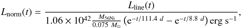 (1)which is independent of distance (as long as the 56Ni mass is estimated assuming the same distance as the line luminosities). For optical lines, Lnorm has in addition only a moderate sensitivity to the extinction as the 56Ni mass is determined in a phase where the bulk of the radiation emerges in the optical bands and thus suffers the same extinction as the optical line luminosity estimates. Instead, the systematic error for Lnorm is dominated by the uncertainty in the 56Ni mass determined for a given distance and extinction.
3.7.1. Error estimates
The meaning of an “error” of a line luminosity measurement depends on the interpretation of these quanties; if one interprets them as particular flux measurements of different parts of the spectrum only the errors in the flux calibration would enter. However, if one desires estimates of actual line luminosities the errors arising from uncertainties in continuum positioning and integration limits enter as well. Here we compute error bars on the data from the second definition, letting them be the rms sum of errors in the photometric flux calibration and line luminosity extractions. The latter component is estimated from visual inspections of the algorithmic fits described above.
4. Overview of modelling results
4.1. Physical conditions
We present here the evolution of some basic physical quantities, using model 13G as an example.
4.1.1. Energy deposition
Figure 1 shows the fraction of radioactive decay energy that is absorbed by the ejecta as a function of time. At 100 days the gamma-ray optical depth is around unity and about half of the gamma-ray energy is absorbed by the ejecta. By 500 days the optical depth has dropped by a factor of 25 and only a small percent of the gamma-ray energy is absorbed by the ejecta. By this time the positrons (which are fully trapped) contribute about as much power as the gamma rays.
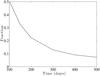 |
Fig. 1 Fraction of radioactive decay energy (gamma rays and positrons) deposited in the ejecta, for model 13G. |
4.1.2. Temperature
Figure 2 shows the temperature evolution in various zones for model 13G. The Fe/Co/He zone temperature refers to the core component, the He/C and He/N temperatures to the innermost He envelope components, and the H temperature to the innermost H envelope component.
The hottest zones are the He/N zones which contain small amounts of effective coolants, having helium (an inefficient coolant) as 99% of the composition. Most cooling is done by N II and Fe III. The He/C zones are somewhat coolant (especially at early times) as a result of the efficient cooling by C II. At later times Ne II is the main coolant. The coldest zone is the Si/S zone, which contains only small amounts of 56Ni, has intermediate density, and has a good cooling capability through mainly Ca II, but also from Si I, S I, and Fe II at later times. Although they have a high cooling capability, the low density combined with the local positron absorption of model 13G make the Fe/Co/He clumps quite hot. The most prominent coolants are Fe II, Fe III, and Co II (whose contribution steadily declines with time as it decays). In the O/Ne/Mg zone, Fe II and Mg II are initially important coolants, but after 150 days O I is the strongest coolant with a contribution of 30−75%. Finally, the cooling of the H zones is dominated by Mg II, N II, and Fe II.
We note that the cooling situation can only be analysed locally. Some of the cooling radiation is reabsorbed by the zone (particularly lines at short wavelengths), and the net cooling contributions taking this into account cannot be directly accessed.
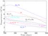 |
Fig. 2 Temperature evolution in selected zones, model 13G. |
4.1.3. Ionization
Figure 3 shows the evolution of the electron fraction xe = ne/nnuclei, where ne is the electron number density and nnuclei is the number density of nuclei. The low-density core zones (Fe/Co/He and Si/S) obtain electron fractions of xe ~ 1, whereas the higher-density core zones (O/Si/S, O/Ne/Mg, O/C) as well as the envelope zones (He/C, He/N, H) have xe ~ 0.1.
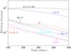 |
Fig. 3 Evolution of electron fraction xe in selected zones, model 13G. |
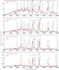 |
Fig. 4 SN 2011dh (dereddened and redshift corrected) at 99 days (top), 202 days (second panel), 293 days (third panel), and 415 days (bottom) (red) and model 12C at 100, 200, 300, and 400 days (black), scaled with exponential factors exp(−2Δt/ 111.4), where Δt is the difference between observed and modelled phase (here Δt = −1, +2, −7, +15 days). The decay rate of double the 56Co rate corresponds to the flux evolution in most photometric bands (E14b). The most distinct emission lines are labelled with their dominant contributing element in the model. |
4.2. Model spectra
Figures 4−8 show selected comparisons between observed spectra of SN 2011dh, SN 2008ax, and SN 1993J and model spectra.
Of the models presented in Table 3, model 12C (MZAMS = 12 M⊙, strong mixing, local positron absorption, no molecular cooling, dust formation at 200 days, and χ = 210) shows good overall agreement with the spectral evolution of SN 2011dh (Figs. 4, 5). In particular, this model reproduces accurately the evolution of the [O I] λλ6300, 6364 doublet (Fig. 15), which is an important diagnostic of the progenitor mass (see Sect. 5.5).
Models 13G and 17A, the analogues of 12C at higher MZAMS, are compared with SN 2008ax and SN 1993J in Figs. 6−8. These show fair agreement, although the oxygen lines in SN 1993J suggest a MZAMS value of somewhere between 13 and 17 M⊙. Both observed and modelled spectra will be discussed in more detail in Sect. 5, where we study line formation element by element.
4.2.1. Evidence for dust in SN 2011dh
In Fig. 5 we show that a dust component is necessary to reproduce the NIR spectrum of SN 2011dh at 200 days. A thorough analysis of this dust component, including modelling of mid-infrared data (which supports the dust hypothesis), is presented in E14b. Figure 6 shows that the last NIR spectrum of SN 2008ax at 130 days showed no such dust component; any dust formation in this SN must therefore have occurred later.
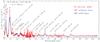 |
Fig. 5 SN 2011dh (dereddened and redshift corrected) in the NIR at 200 days (red). The observed spectrum is composed of 1−1.5 μm observations at 198 days scaled with exp(−2 × 2 / 111.4) and 1.5−2.5μm observations at 206 days, scaled with exp( + 2 × 6 / 111.4). Also plotted is model 12C without (blue dashed) and with (black solid) a dust component (τ = 0.25, xdust = 0.05). Line identifications from the model are labelled. A dust component clearly improves the fit above 1.5 μm. |
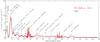 |
Fig. 6 SN 2008ax (dereddened and redshift corrected) in the NIR at 130 days (red) and model 13G at 150 days (black) (rescaled with exp( + 2 × 20 / 111.4) to compensate for the different epoch and with a factor of 1.33 to compensate for the higher 56Ni mass). Line identifications from the model are labelled. |
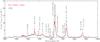 |
Fig. 7 SN 1993J (dereddened and redshift corrected) at 283 days (red), and model 17A at 300 days (black) (rescaled with exp( + 2 × 17 / 111.4) to compensate for the different epoch and with a factor of 1.2 to compensate for the higher 56Ni mass). |
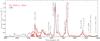 |
Fig. 8 SN 2008ax (dereddened and redshift corrected) at 280 days (red), and model 13G at 300 days (black) (rescaled with exp( + 2 × 20 / 111.4) to compensate for the different epoch and with a factor of 1.33 to compensate for the higher 56Ni mass). |
5. Line formation element by element
5.1. Hydrogen lines
The hydrogen envelope of 0.1 M⊙ receives little of the energy input from 56Co, typically around 0.5% of the total deposition at all epochs in the 100−500 day range. This is too little to produce any detectable emission from Hα or from any other lines in our models. The only influence of the hydrogen envelope is to produce an Hα scattering component at early times (Fig. A.8), but that too disappears after ~150 days as the Balmer lines become optically thin. Our conclusion is therefore that the hydrogen envelope cannot affect the spectrum by emission or absorption by H lines after ~150 days. This result is in agreement with the SN 1993J analysis by Houck & Fransson (1996), who found that the Hα emission in their models was inadequate to account for the observed flux around 6550 Å.
A strong line around 6550 Å is nevertheless seen for much longer into the nebular phase for the SNe studied here. In our models, a strong line in this spectral region is produced by [N II] λλ6548, 6583, arising as cooling lines from the He/N layers (Sect. 5.4, Fig. 9). In the Houck & Fransson (1996) models N II was not included, and the inclusion of this ion in the models presented here resolves the apparent discrepancy regarding the nature of the 6550 Å feature.
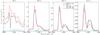 |
Fig. 9 Same as Fig. 4, zoomed in at 6000−7000 Å, and also showing the contributions by [N II] λλ6548, 6583 (blue), Hα (green), and Hα multiplied by 10 (dashed green) to the model spectrum. After 200 days, the [N II] λλ6548, 6583 lines are fully responsible for the feature between 6400−6700 Å. |
5.1.1. Time-dependence
Some caution is needed when drawing conclusions from steady-state modelling of Hα, because the dilute hydrogen envelope is the first region to be affected by time-dependent effects. Figure 10 shows the ratio of recombination time τrec3 to radioactive decay timescale τ56Co = 111.4 d, and the cooling timescale τcool relative to τ56Co, in the inner hydrogen envelope shell in model 12C. We see that breakdown of the steady-state assumption (that both of these ratios are ≪1, see Jerkstrand 2011) begins at 150−200 days. This breakdown will lead to temperature and ionization balance differing from those obtained in steady-state calculations (Fransson & Kozma 1993), and time-dependent modelling is needed for highest accuracy. We note, however, that the ionization level in the steady-state model is xHII ~ xe ≳ 1 / 4 over the 100−300 day interval (Fig. 10) and so even in a situation of complete ionization (xHII ~ xe ~ 1), the recombination contribution to Hα could be at most a factor of ~16 stronger (as the total number of recombinations per unit time scales with xHII·xe). As Fig. 9 shows, this would still be too little to match the observed luminosity. It therefore appears to be a robust result that 56Co-powered Hα is undetectable after ~150 days in Type IIb SNe.
5.1.2. Early-time Hα scattering
Before ~150 days, Hα is optically thick in the inner hydrogen envelope and will affect the spectrum with absorption (Houck & Fransson 1996; Maurer et al. 2010). If the bulk of the photons are emitted from a core region with a velocity scale much smaller than the expansion velocity VH of the H-envelope “shell” (where Hα is optically thick), this absorption will be in the form of a band centred at λc ~ 6563 × (1 − VH/c) ~ 6320 Å (using VH = 1.1 × 10⁴ km s-1), with a width governed by the velocity distribution of both the hydrogen shell and the emitting region. The width will roughly correspond to the larger of these velocity scales. Since they are both on the order of a few thousand km s-1, the width of the absorption band will be Δλ ~ λc2ΔV/c ~ 150 Å, where we have used ΔV ~ 3500 km s-1.
The absorption band is seen in the models at 100 days (Figs. 4 and 9). The absorption begins around 6350 Å, (≈λc + 1 / 2Δλ = 6390 Å), reaches maximum strength at 6315 Å (≈λc = 6320 Å), and ceases at 6260 Å (≈λc−1 / 2Δλ = 6250) Å. The observed profile shows a similar structure, with a minimum at 6325 Å, a cut-off to the blue at 6275 Å, but no clear cut-off to the right. The region is complex, with an [Fe II] line contributing on the red side as well. The absorption in the model is stronger than in the observed spectrum, and it is therefore unlikely that the hydrogen density in the model is underestimated. Finally, we note that Hβ and the other Balmer lines are optically thin in the model in the time interval studied here, and therefore do not produce similar absorption bands (which would be centred at ~4680 Å and ~4180 Å for Hβ and Hγ.)
5.1.3. Circumstellar interaction Hα
That radioactivity is unable to power Hα in the nebular phase of Type IIb SNe is a result previously discussed by Patat et al. (1995), Houck & Fransson (1996), and Maurer et al. (2010). That a strong emission line around 6550 Å is nevertheless often seen in nebular Type IIb spectra is usually explained by powering by X-rays from circumstellar interaction. Although that process undoubtedly occurred after about a year for SN 1993J, it has proven difficult to quantitatively reproduce the luminosity and line profile evolution at earlier times (Patat et al. 1995, T11). In particular, a circumstellar interaction powered Hα does not produce an emission line profile as narrow as observed, as hydrogen is confined to velocities ≳104 km s-1 (Sect. 3.2.3).
In SN 1993J, circumstellar interaction started dominating the output of the SN after about a year, leading to a leveling off in all photometric bands to almost constant flux levels (e.g. Zhang et al. 2004). The 6500−6600 region then became dominated by Hα from circumstellar interaction, showing a broad and boxy line profile with almost constant flux (Filippenko et al. 1994; Patat et al. 1995; Houck & Fransson 1996). This interpretation was validated by similar Hβ and Hγ emission lines emerging in the spectrum. No such flattening was observed in SN 2011dh, at least up to 500 days, and the spectral region continues to be dominated by the [N II] λλ6548, 6583 lines from the ejecta.
5.2. Helium lines
Helium line formation in the nebular phase is complex, as He is present in several compositionally distinct regions in the SN. CNO burning leaves the progenitor with a He/N layer enriched in nitrogen and depleted in carbon. The inner parts of this zone are subsequently processed by incomplete (shell) helium burning, which destroys the nitrogen and burns some of the helium to carbon. The resulting He/C layer is then macroscopically mixed to an uncertain extent into the core as the O/C-He/C interface gives rise to a Rayleigh-Taylor unstable reverse shock (Iwamoto et al. 1997). Alpha-rich freeze-out in the explosive burning also leaves a large mass fraction (20−50 %) of He in the 56Ni clumps. Despite the much lower mass of He in these clumps compared to the He/N and He/C zones, this He can contribute to the total He line emission if local trapping of the radioactive decay products is efficient (e.g. Kjær et al. 2010).
He-line analysis must thus consider contributions from three distinct zones (and possibly from the He in the H envelope as well). We find that in general all three of the He/N, He/C, and Fe/Co/He zones contribute to the He lines (Figs. A.6−A.8).
5.2.1. He I λ1.083 μm and He I λ2.058 μm
In Fig. A.1 we plot the contribution of He lines to the 13G model spectrum at 100, 300, and 500 days. At all epochs, He I λ1.083 μm is the strongest He emission line in the models. There is some blending of this line with [S I] λ1.082 μm (Fig. A.3), particularly at late times. This blending was also established for SN 1987A (Li & McCray 1995; Kozma & Fransson 1998), and the presence of a strong line around 1.08 μm also in nebular spectra of Type Ic SNe has been explained by this sulphur line (Mazzali et al. 2010). He I λ2.058 μm does not suffer from any significant line blending in the models, and detection of this line therefore appears less ambiguous for establishing the presence of He in the SN ejecta.
The lower levels of the He I λ1.083 μm and He I λ2.056 μm lines (2s(3S) and 2s(1S), respectively) are meta-stable. Having only weak radiative de-excitation channels to the ground state (A = 1.1 × 10⁻⁴ s-1 and A = 51 s-1 (two-photon), respectively), these level populations become quite high, being limited by excitation and ionization processes rather than radiative de-excitation. The result is significant optical depths in the transitions; they are both optically thick throughout the helium envelope at 200 days. This optical depth means that both lines have scattering components, which are also seen in the observed lines in SN 2011dh at 88 days (E14a) and 200 days (Fig. 5). At later times He I λ1.083 μm stays optically thick, whereas He I λ2.058 μm becomes optically thin (Fig. 12) as the two-photon decay channel becomes significant.
The populations of the meta-stable levels are high enough that some cooling occurs from them through collisional excitatons to higher states. In general the He I λ1.083 μm and He I λ2.058 μm lines have contributions from scattering, recombination, non-thermal excitation, and collisional excitation. Figure 11 gives some insight into the formation of these lines by showing the various populating processes in the innermost He/N shell in model 13G between 100−300 days. The He I λ2.058 μm line is mainly driven by cascades from levels above as well as some thermal excitation at early times and non-thermal excitations at later times. The situation is somewhat different for He I λ1.083 μm. Its parent state has a much smaller high-energy collisional cross section with respect to the ground state and non-thermal excitations are negligible. There is instead an important contribution by thermal collisional excitation from 2s(3S). The cooling done by this transition is typically a few percent of the total cooling of the He/N layers. Cooling through the He I λ2.058 μm channel is less efficient, especially at late times, because the 2s(1S) state has in general a significantly lower population than 2s(3S), as it can be emptied via two-photon decay with A = 51 s-1 (the two-photon decay channel of 2s(3S) is inefficient (A ~ 10-9 s-1, Li & McCray 1995).
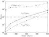 |
Fig. 10 Recombination (solid) and cooling (dashed) timescales relative to the 56Co decay timescale, and the quantity |

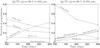 |
Fig. 11 Relative importance of processes that populate the parent states of He I λ1.083 μm and He I λ2.058 μm, in the innermost He/N shell in model 13G. |
Model 12C gives a reasonable reproduction of the He I NIR lines in SN 2011dh at 200 days, although the observed lines have more flux at line center (Fig. 5). For the 1.08 μm feature, it is possible that this contribution is from [S I] λ1.082 μm rather than He I 1.083 μm. Model 13G (which has very similar He lines) gives good agreement with SN 2008ax at 130 days (Fig. 6), which has more of a flat-topped He I λ1.083 μm line. Both these SNe are therefore in good agreement with models having ~1 M⊙ of helium in the ejecta.
5.2.2. Optical helium lines
In the optical, the strongest lines in the models are He I λ5016, He I λ6678, and He I λ7065 (Fig. A.1). All of these are present in the spectrum of SN 2011dh at 100 days (Fig. 4). At later times they quickly diminish in strength and are harder to detect. Figure 12 shows how the optical depths in He I λ5016 and He I λ3889 stay high in the nebular phase; the reason is that these lines have one of the meta-stable states as the lower level. He I λ3889 and He I λ5016 are thus expected to have the strongest absorption components in the optical regime. Whereas He I λ3889 absorption is difficult to disentangle from Ca II HK aborption, a distinct scattering component of He I λ5016 is seen up to 200−300 days in SN 2011dh (Fig. 4). In-depth modelling of this line may be able to further constrain the helium mass and distribution.
He I λ4471, He I λ5876, He I λ6678, and He I λ7065 do not have meta-stable lower states, and although some are still optically thick at 100 days, by 150 days they are all optically thin. One consequence is that the absorption seen around 5800 Å (Fig. 4) is not due to He I λ5876 after 150 days, but rather due to Na I-D. He I λ5876 emission also does not emerge directly in the model, as most of its flux scatters in these Na I-D lines (Sect. 5.6).
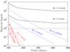 |
Fig. 12 Optical depths of He I lines over time, in the innermost He/N envelope shell of model 12C. Lines with the meta-stable 2s(3S) as the lower level are marked in solid black, lines with the meta-stable 2s(1S) as the lower level are marked in dashed blue, and lines with non-metastable lower levels are marked in dash-dotted red. |
5.3. Carbon lines
Figure A.1 (bottom panel) shows the contribution by C I to the spectrum (the contribution by other carbon ions is neglegible). At all times there is only significant emission redward of ~8000 Å. At 100 days there is a large number of intermediate strength lines, but later on the C I spectrum is dominated by two features; [C I] λ8727 and [C I] λλ9824, 9850. A few times weaker but still possible to detect are C I λ1.176 μm and C I λ1.454 μm. The C I emission is mainly from the carbon in the O/C zone, but there is also a small contribution from the carbon in the He/C zone (Fig. A.7).
The presence of either [C I] λ8727 or [C I] λλ9824, 9850 in the observed spectra is difficult to ascertain; [C I] λ8727 is blended with the strong Ca II λ8662 line, and the spectral region covering [C I] λλ9824, 9850 has poor observational coverage. In SN 2008ax, the day 280 spectrum covers the region, and shows a feature that coincides with the line (Fig. 8). Spectra of SN 2011dh at 360 and 415 days cover the wavelength regime, but are noisy and difficult to interpret.
Both [C I] λ8727 and [C I] λλ9824, 9850 are cooling lines, and are therefore sensitive to CO formation in the O/C zone which can dramatically change the temperature. Without CO, the [C I] lines are strong because a significant amount of cooling occurs through them. In model 13G, the neutral fraction of carbon is 0.26, 0.75, and 0.88 at 100, 300, and 500 days, and C I does ~20% of the cooling. CO formation could quench these lines as even small amounts of CO would take over most of the cooling (Liu & Dalgarno 1995). Model 12C (which has no CO cooling) makes a good reproduction of the Ca II IR + [C I] λ8727 blend at 200 days, but there is then a growing overproduction with time (Fig. 4), possibly as CO cooling becomes more and more important. Models with full CO cooling have the opposite problem, with an underproduced [C I] λ8727 line at early times (Sect. 7.4).
5.4. Nitrogen lines
5.4.1. [N II] λλ6548, 6583
As discussed in Sect. 5.1, cooling of the He/N zone by [N II] λλ6548, 6583 is responsible for almost all emission in the 6400−6800 Å range in the models, exceeding the Hα contribution by large factors after 150 days (Fig. 9). The nitrogen lines naturally obtain somewhat flat-topped profiles as most of the He/N layers expand with high velocities (3500−11 000 km s-1, which formally gives a flat-topped region between 6470−6660 Å), but an important distinction to the Hα component is that Hα obtains a significantly broader flat-top (~6320−6800 Å), since H is confined to V> 11 000 km s-1.
Figures 4 and 8 show that the observed line profiles in SN 2011dh and SN 2008ax have flat-topped parts extending out to ~6600−6650 Å on the red side, in better agreement with an interpretation as originating in the He envelope than in the H envelope. This discrepancy for interpreting the emission in this range with Hα has been pointed out by T11. Figure 7 shows that SN 1993J has a flat-topped part that extends to somewhat longer wavelengths (~6700 Å), and combined with the lower H velocities in this SN the interpretation is more ambiguous.
The models reproduce the [N II] λλ6548, 6583 feature in SN 2011dh quite well, both in terms of luminosity and line profile (Fig. 9). The observed profile is initially flat-topped (as in the models), but becomes less so with time; this possibly indicates that some of the He/N zone is mixed into the core (the models have only a mixed-in He/C component). Reasonable reproduction is also achieved for SN 1993J and SN 2008ax (Figs. 7 and 8). However, by 400 days Hα has completely taken over in SN 1993J (Fig. 13) as a result of strong circumstellar interaction; note how the line profile expands to a flat-topped region out to 6750 Å (Vexp ~ 9000 km s-1). After ~400 days, the model starts overproducing the [N II] λλ6548, 6583 doublet compared to observations of SN 2011dh. While adiabatic cooling is still only 1−12% in the various He/N layers at 300 days, by 400 days it has reached 3−26%, and the steady-state assumption starts breaking down in the outer layers.
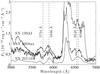 |
Fig. 13 5000−7000 Å region at 415 days in SN 2011dh (bottom), SN 2008ax (middle), and SN 1993J (top), all dereddened, redshift corrected, and scaled to the same distance (7.8 Mpc). We identify the feature at ~5700 Å with the blue side of [N II] λ5754, with the red side being lost in scattering into Na I-D. |
Since the [N II] identification is an important result, it is warranted to attempt to understand how robust it is. A first question to consider is the mass and composition of the He/N layer. All WH07 models in the MZAMS = 12−20 M⊙ range have total He zone masses of between 1.0−1.3 M⊙. The fraction that is still rich in N, i.e. has not been processed by helium shell burning, is about 4/5 at the low-mass end and about 1/5 at the high mass end. The mass of the He/N layer thus varies by about a factor of four over the 12−20 M⊙ range, from 0.8 to 0.2 M⊙. The prediction would be, assuming all other things constant, that ejecta from lower mass stars would have stronger [N II] λλ6548, 6583 emission lines.
The nitrogen abundance in the He/N layer is about 1% by mass. The abundances of other possible cooling agents (carbon, oxygen, magnesium, silicon, and iron) are ~0.1%. Helium makes up ~98% of the zone mass, but being a poor coolant itself, the He/N layers are quite hot compared to the other zones. The fraction of the nitrogen that is singly ionized is close to unity in all models at all times, so there should not be any strong sensitivity to the ionization balance. Combining these results (moderate variations in the predicted mass of the He/N layer, a robust prediction for a high temperature, and weak sensitivity of the N II fraction to the ionization balance), strong [N II] λλ6548, 6583 emission appears to be a robust property of the models.
If [N II] λλ6548, 6583 is predicted to be a strong line in the nebular phase of helium-rich SNe, we would expect to see it in both Type IIb and Type Ib SNe. While the emission line is strong in the three Type IIb SNe studied here as well as in the Type IIb SNe 2011ei (Milisavljevic et al. 2013) and 2011hs (Bufano et al. 2014), it appears dim or absent in SN 2001ig (Silverman et al. 2009) and SN 2003bg (Hamuy et al. 2009; Mazzali et al. 2009). Some Type Ib SNe also have spectra that exhibit this line (e.g. SN 1996N (Sollerman et al. 1998) and SN 2007Y (Stritzinger et al. 2009)), while others (e.g. SN 2008D (Tanaka et al. 2009) and SN 2009jf (Valenti et al. 2011)) do not. One possible explanation for the lack of this line in some He-rich SNe could be that the He/N zone (but not the interior He/C zone) has been lost because of stellar winds or binary mass transfer. Another explanation could be that helium shell burning has engulfed most of the He/N layers in these stars and depleted the nitrogen.
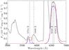 |
Fig. 14 N II emissivity in model 12C at 400 days (red), and the N II photons that emerge in the radiative transfer simulation (blue). Note how much of the [N II] λ5754 emission is absorbed (by Na I D in the He envelope), producing a blueshifted feature as seen in the observed spectra (Fig. 13). Total emergent spectrum is shown in black. |
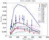 |
Fig. 15 Luminosity in [O I] λλ6300, 6364 normalized to the total 56Co decay power (see Eq. (1)) for SN 1993J, SN 2008ax, and SN 2011dh, and in the models. |
5.4.2. [N II] λ5754
In Fig. A.2 we plot the contribution by nitrogen lines to the spectrum. Apart from [N II] λλ6548, 6583, the only other nitrogen line emitting at detectable levels is [N II] λ5754, which in many ways is analogous to the [O I] λ5577 line (both arise from the second excited state and are temperature sensitive). The red side of this line is scattered by the Na I-D lines (Fig. 14). There is an emission feature in all SN 2011dh spectra centred at ~5670 Å that we identify with this blue edge of [N II] λ5754 (Fig. 4); it is also seen in SN 1993J and SN 2008ax (Fig. 13). The blue edge of the feature extends to ~5600 Å in the observed spectra which would correspond to an expansion velocity of ~8000 km s-1, making an identification with the helium envelope as the source of the emission plausible. Furthermore, in the models Na I-D is optically thick throughout the He envelope during the period studied here (Sect. 5.6). The predicted absorption cut is thus around 5890 Å × (1−1 × 10⁴/ 3 × 10⁵) ~ 5700 Å (see also Fig. 14), in good agreement with the observed line.
The [N II] λ5754 model luminosity at 400 days matches the observed value reasonably well, although the line profile is too narrow (Fig. 4). No other emission lines are produced by the models in the relevant range, further strengthening the identification. However, at 200 and 300 days the line is too strong (Fig. 4). As [N II] λ5754 is temperature sensitive, this is likely caused by a He/N zone model temperature that is too high. The model temperatures are between 10 000−12 000 K in the various He/N shells at 200 days. Inspecting the temperature sensitivity of the Boltzmann factor that governs these thermally excited lines, a lower temperature by 1500 K would decrease [N II] λ5754 by a factor of 2, and a 3000 K decrease would decrease it by a factor of 5, whereas [N II] λλ6548, 6583 would only change by factors of 1.3 and 2, respectively. Since [N II] λ5754 is more temperature sensitive than [N II] λλ6548, 6583, a lower temperature would decrease or eliminate [N II] λ5754 while affecting [N II] λλ6548, 6583 less (compare to how [O I] λ5577 rapidly disappears as the SN evolves while [O I] λλ6300, 6364 persists). Thus, the model overproduction of [N II] λλ5754 does not per se invalidate the [N II] λλ6548, 6583 identification.
5.5. Oxygen lines
The oxygen lines that emerge in the models are [O I] λ5577, [O I] λλ6300, 6364, O I λ77744, O I λ92635, O I λ1.129 μm + O I λ1.130 μm, and O I λ1.316 μm (Fig. A.2). Inspection of the various populating mechanisms shows that [O I] λ5557 and [O I] λλ6300, 6364 are mainly driven by thermal collisional excitation at all times, as they are close to the ground state and in addition radiative recombination to singlet states from the O II ground state is forbidden. The O I λ7774, O I λ9263, O I λ1.129 + λ1.130 μm, and O I λ1.316 μm lines are instead mainly driven by recombination.
5.5.1. [O I] λλ6300, 6364
Figure 15 shows the luminosity of [O I] λλ6300, 6364 (relative to the 56Co decay power) for SN 2011dh, SN 2008ax, and SN 1993J6, and in the models. All three SNe show luminosities in this line that are bracketed by the model luminosities from MZAMS = 12−17 M⊙ progenitors, for which the oxygen mass range is MO = 0.3−1.3 M⊙. SN 1993J has the brightest normalized oxygen luminosity, roughly halfway between the 13 and 17 M⊙ models, suggesting a ~15 M⊙ progenitor (MO = 0.8 M⊙). In the WH07 models, oxygen production grows sharply for progenitors over ~16 M⊙, and as the comparison with the 17 M⊙ model shows, none of these SNe exhibit the strong [O I] λλ6300, 6364 lines expected from the ejecta from such high-mass stars. Figure 7 shows model 17A compared to SN 1993J at 300 days; there is reasonable overall agreement with this model, but the model oxygen lines are too strong by about a factor of two.
An important quantity to attempt to constrain is the oxygen zone density, which is possible if the optical depths of the [O I] λλ6300, 6364 lines can be determined. In SN 1987A, the [O I] λλ6300, 6364 lines began to depart from the optically thick 1:1 regime at 100 days, and passed τ6300 = 1 around 400−500 days (Spyromilio & Pinto 1991; Li & McCray 1992). Since the expansion velocities here are about a factor of two higher, the densities for a similar oxygen mass and filling factor are a factor of eight lower. As the optical depths evolve as t-2, the τ6300 = 1 limit is then expected to be reached by 400/ days instead of 400 days.
Since the expansion velocity of the metal core of the SN is greater than the 3047 km s-1 separating the [O I] λ6300 and [O I] λ6364 lines, the two lines are blended and the individual components of the doublet cannot be directly extracted. Figure 16 shows the best fit to the doublet line profile in SN 2011dh for an optically thin (black) and an optically thick (blue) model with Gaussian components. The optically thin version gives a better fit at all times, although at 100 days neither fit is good, likely as a result of line blending and radiative transfer effects (see Sect. 6 for more on this). If we take the lines to have entered the optically thin regime at 150 days, and use the Sobolev expression for the optical depth (ignoring the correction for stimulated emission) 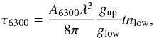 (2)we obtain, with A6300 = 5.6 × 10⁻³ s-1, λ = 6300 × 10-8 cm, gup = 5 (the statistical weight of the upper level), glow = 5 (the statistical weight of the lower level), and
  7 an upper limit to the density of the oxygen of ρO< 7 × 10-14 g cm-3 at 150 days. This limit is satisfied by all the models computed here, which have ρO between (1−5) × 10-14 g cm-3 at 150 days. For the oxygen masses in the ejecta from 12, 13, and 17 M⊙ progenitors (0.3, 0.5, and 1.3 M⊙), the density limit corresponds to filling factor limits fO ≳ 0.02,0.04 and 0.09 (for Vcore = 3500 km s-1).
An additional constraint on the oxygen zone filling factor from small-scale fluctuations in the line profiles is derived in E14b; this analysis gives a constraint fO< 0.07, which is already in tension with the minimum filling factor needed for the 17 M⊙ model to reproduce the [O I] λλ6300, 6364 optical depths. Independent of luminosity, these constraints from the line-profile structure of [O I] λλ6300, 6364 therefore constrain the thermally emitting oxygen mass in SN 2011dh to less than 1.3 M⊙.
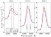 |
Fig. 16 [O I] λλ6300, 6364 feature in SN 2011dh, dereddened and redshift corrected (red), and the best double Gaussian fits assuming optically thin (3:1) (black solid line) and optically thick (1:1) (blue dashed line) emission. Both fits are poor at 99 days, at 152 and 202 days the optically thin fits are superior. |
5.5.2. [O I] λ5577 and the [O I] λ5577/[O I] λλ6300, 6364 ratio
The [O I] λ5577 line arises from 2p4(1S) which is 4.2 eV above the ground state and is efficiently populated by thermal collisions in the early nebular phase, when the temperature is high. Since both [O I] λ5577 and [O I] λλ6300, 6364 are driven by thermal collisions at all times, the [O I] λ5577/[O I] λλ6300, 6364 ratio can serve as a thermometer for the oxygen region. Two effects complicate this simple diagnostic, however; at early times line blending and radiative transfer effects make it difficult to assess the true emissivities in the lines (Sect. 6), and at later times, when these complications abate, the [O I] λ5577 line emission falls out of LTE, which introduces an additional dependency on electron density.
Figure 17 shows the luminosity in [O I] λ5577 and the ratio [O I] λ5577/[O I] λλ6300, 6364. It is noteworthy how similar the evolution of this line ratio is in the three SNe. Most of the models overproduce this ratio by a factor of ~2. Since both lines are driven by thermal collisions, one possible reason for this is that the oxygen-zone temperatures are too high in the models. This in turn must be caused by either a too close mixing between the gamma ray emitting 56Ni clumps and the oxygen clumps, or an underestimate of the cooling ability of the oxygen zones.
The cooling efficiency has some dependency on the density; a higher density leads to more frequent collisions, which increases the efficiency of collisional cooling, but it also leads to higher radiative trapping, which reduces the efficiency of the cooling. Comparing models 13C and 13E, which only differ in density contrast factor χ, model 13E (which has a higher χ and therefore a higher O-zone density) has a higher O/Ne/Mg zone temperature (6060 K vs. 5860 K at 150 days), suggesting that the second effect dominates at this time. We note, however, that there may also be other effects involved, for example is the ionization balance dependent on density, and different ions have different cooling capabilities. Apart from the temperature effect, a higher density also brings the [O I] λ5577 parent state closer to LTE (departure coefficient 0.8 instead of 0.5), and the combined effect is a higher [O I] λ5577/[O I] λλ6300, 6364 line ratio (the parent state of [O I] λ6300, 6364 is in LTE in both scenarios). From this comparison, a high O-zone density is not favoured by the [O I] λ5577/[O I] λλ6300, 6364 line ratio. This is however not consistent with the constraints imposed by the fine structure analysis of the oxygen lines (E14b) and by magnesium recombination lines (Sect. 5.7). This suggests that a too strong mixing between the 56Ni clumps and the oxygen clumps is more likely to explain the [O I] λ5577/[O I] λλ6300, 6364 line ratio discrepancy. Other factors, such as line blending, line blocking (see Sect. 6), and molecular cooling may, however, also affect the line ratio. As Fig. 26 shows, there is [Fe II] emission contaminating both [O I] λ5577 and [O I] λλ6300, 6364 (at least at 100 days), and the discrepancy may be related to this line blending.
In Table 5 we report the measured line ratios, derived LTE temperatures, and O I masses from the [O I] λ5577 and [O I] λλ6300, 6364 luminosities (using Eqs. (2) and (3) in Jerkstrand et al. 2014), which assume optically thin emission and no blending or blocking. The errors are estimated using the linearized error propagation formula. From the spectral models we find an epoch of around 150 days to be the most relevant for the application of this method; before this time the lines are significantly blended and/or blocked, and at later times the [O I] λ5577 line starts to deviate strongly from LTE. That the oxygen masses determined with this method are roughly consistent with the ones inferred from the detailed spectral synthesis modelling (Sect. 5.5.1) means that the factor of ~2 difference in the [O I] λ5577/[O I] λλ6300, 6364 ratio between the observations and models does not translate to any large differences in the derived oxygen masses.
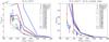 |
Fig. 17 Left: luminosity in [O I] λ5577 relative to the 56Co decay power in the models and in SN 1993J, SN 2008ax, and SN 2011dh. Right: [O I] λ5577/[O I] λλ6300, 6364 line ratio. |
Measurements of the [O I] λ5577 / [O I] λλ6300, 6364 line ratio in SN 1993J, SN 2008ax, and SN 2011dh; the derived LTE temperature (assuming optically thin emission); and the thermally emitting O I mass (with the same assumptions).
5.5.3. Oxygen recombination lines
There are four recombination lines predicted as being detectable and which also appear to be detected in the spectra of SN 2011dh: O I λ7774, O I λ9263, O I λ1.129 μm + O I λ1.130 μm, and O I λ1.316 μm (Figs. 18, A.2)8. These are allowed transitions from high-lying states (excitation energies >10 eV) which cannot be populated by thermal collisions from the ground state. Inspection of the solutions for the non-thermal energy deposition channels shows that, at all epochs, at least ten times more non-thermal energy goes into ionizing oxygen than exciting it. Emission lines from high-lying states are thus to a larger extent driven by recombinations than by non-thermal excitations. This result was also obtained by a similar calculation by Maurer & Mazzali (2010).
Letting ψ denote the fraction of the electrons that are provided by oxygen ionizations (ψ = nOII/ne), the recombination line luminosity of a transition ul is 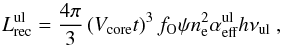 (3)where fO is the oxygen zone filling factor, and u and l refer to the upper and lower levels. The factor ψ is close to unity at early times (as oxygen dominates the zone composition and ionization is relatively high), for our models we find ψ ≈ 0.5 between 100−200 days in the O/Ne/Mg zone. The effective recombination rates
  are (for the purpose of the analytical formulae here) computed in the purely radiative limit (no collisional de-excitation), using Case B for the optical depths (see Appendix C for details). These are considered accurate as recent calculations of the recombination cascade of O I have been presented (Nahar 1999).
We analyse the models for the amount of line blending and/or scattering that is present for each of the four recombination lines. The presence of blending and scattering still allows a determination of an upper limit to the recombination luminosity of the line of interest, which from Eq. (3) translates to an upper limit for  .
.
In the models, O I λ7774 is relatively uncontaminated, but is optically thick (in the oxygen zones) up to ~400 days, so pure recombination emission, i.e. when blending with other lines is weak and no populating mechanisms other than recombination (e.g. scattering) are important, is present only after this time. O I λ9263 is at all times blended with in particular [Co II] λλ9336, 9343, but also with S I λλ9213, 9228, 9237 and Mg II λλ9218, 9244 at early times. It becomes optically thin around 200 days. Pure recombination emission is never present.
The O I λ1.129 + λ1.130 μm feature has little contamination in the model at 100 and 150 days, but from 200 days and later [S I] λ1.131 μm contaminates. Na I λλ1.138, 1.140 μm also contributes in the red wing, with a typical luminosity of ~10% of the oxygen line. The O I λ1.129 + λ1.130 μm lines become optically thin at ~200 days. Pure recombination emission is never present. The O I λ1.316 μm line has little contamination in the model early on, but for t ≳ 200 days becomes overtaken by [Fe II] λ1.321 μm + [Fe II] λ1.328 μm (Fig. A.4). It becomes optically thin at around 150 days. Pure recombination emission is present between ~150−200 days.
 |
Fig. 18 Models with low (13C, black) and high (13E, blue) density in the oxygen regions show similar O I recombination line luminosities, here at 200 days. Observed spectrum of SN 2011dh (optical part: 202 days, NIR part: 198 days) in red (dereddened and redshift corrected). |
We use these considerations to derive either direct estimates (when pure recombination is indicated) or upper limits (when blending and/or scattering is indicated) of the quantity  , presented in Table 6. All recombination lines give fairly consistent values of
  , which for ψ = 0.5 are
  cm-3 at 100 days and
  cm-3 at 200 days.
The quantity is not expected to have any strong dependency on fO; doubling the volume (i.e. increasing  by a factor
  ) leads to (approximately) a factor of two reduction of ionization rates per unit volume, which under the steady-state constraint must lead to a factor of two reduction of the recombination rates per unit volume (
 . If ψ stays constant, this means a factor of two reduction in
  , i.e. a factor of reduction in ne, and stays constant.
This is confirmed by comparing models 13C and 13E with respect to the oxygen recombination lines; their luminosities are similar despite a factor of 5 different fO values (Fig. 18). The low density model 13C has (for the O/Ne/Mg zone) fO = 0.13 and obtains an electron density ne = 5.5 × 107 cm-3, so  cm-3. The high density model 13E has fO = 0.026 and obtains ne = 1.5 × 108 cm-3, so
  cm-3, almost the same.
From Figs. 4 and 5 it can be seen that O I λ7774 and O I λ9263 are satisfactorily reproduced by model 12C at 100 days, but that O I λ7774, O I λ1.129 μm + λ1.130 μm, and O I λ1.316 μm are underproduced at 200 days (O I λ9263 is hard to ascertain because of blending with [Co II] λλ9336, 9343). At this time, the O/Ne/Mg zone has nef1 / 2 = 1.5 × 107 cm-3. The O/Si/S and O/C zones have similar values and the total nef1 / 2 value is therefore close to the required 3 × 107 cm-3 derived above, so we would expect the recombination lines to be accurately reproduced. The reason for the discrepancy lies in the ψ factor. Closer inspection of the ionization balance at 200 days shows that the O II ions in the O/Si/S and O/C zones have been completely neutralized by charge transfer with Si I, S I, and C I (reactions that are much more rapid than radiative recombination), and ψ ≪ 1 in these zones. The ion pools instead consist of Mg II, Si II, and S II (O/Si/S zone) and C II and Mg II (O/C zone). If these charge transfer reactions are overestimated, the recombination lines from O I become underestimated.
The critical charge transfer reactions are O II + Si I, O II + S I, O II + C I, and O II + Mg I, as all other species in the oxygen zones are too rare to affect the pool of oxygen ions. To our knowledge, no published calculations for these rates exist. We use fast reactions rates of 10-9 cm3 s-1 for the first three, and a slow reaction rate (10-15 cm3 s-1) for the last; this treatment is based only on the presence or absence of transitions with typical resonance values (Rutherford et al. 1971; Pequignot & Aldrovandi 1986).
The uncertainty in these charge transfer rates affects the oxygen ionization balance mainly in the O/Si/S and O/C zones, which are rich in Si/S and C, respectively. Since the O/Si/S and O/C zones contain about 2/3 of the oxygen mass in low-MZAMS models, this gives a factor of ~3 uncertainty in the O I recombination line luminosities. This roughly corresponds to the underproduction of the O I recombination lines in 12 M⊙ models at 200 days, and we therefore do not consider this discrepancy to be critical. At higher MZAMS, the fraction of the oxygen that resides in the O/Ne/Mg zone increases, and this reduces the uncertainty in the “effective” ψ.
Charge transfer also makes dependent on fO, because charge transfer neutralization of O II operates more efficiently at higher densities for which there are more neutral Si, S, and C atoms available per oxygen ion. Looking again at models 13C and 13E at 200 days, ψ in the O/Ne/Mg zone decreases from 0.63 at low density (13C) to 0.37 at high density (13E), as charge transfer neutralization of O II is more efficient in the high-density case. In the O/C zone, O II is fully neutralized in both models (ψ< 1 × 10⁻³), whereas in the O/Si/S zone ψ = 0.31 in 13C and ψ = 1.2 × 10⁻³ in 13E. The result is that, past some threshold, charge transfer neutralization of O II can cause O I recombination lines to become weaker with increasing density.
5.6. Sodium lines
Sodium has only one strong line throughout the optical/NIR region; the Na I D doublet (Fig. A.2). The Na I λλ1.138, 1.140 μm line may be detectable but it is quite weak in the models here.
Even small amounts of Na I can produce optically thick D-lines throughout a SN nebula for a long time, giving a strong P-Cygni component. Any He I λ5876 emission would scatter in these optically thick D-lines. In model 12C, the Na I D lines are optically thick throughout most of the helium envelope over the whole 100−500 day interval. The optical depths in fact increase with time as the neutral fraction of sodium grows faster than t2, the rate at which the Sobolev optical depths decrease with time for a constant number of atoms. For example, the neutral fraction of sodium in the outermost He shell is 1.5 × 10⁻⁵ at 100 days and 1.4 × 10⁻³ at 500 days, a 100-fold increase compared to a factor of 25 drop in t-2.
The location in the helium envelope outside which the Na I lines become optically thin goes from ~7500 km s-1 at 100 days to ~9000 km s-1 at 500 days (model 12C). A distinct absorption trough from ~5890 Å × (1−9000 / 3 × 10⁵) = 5710 Å is produced, which is clearly seen in observed spectra, particularly at early times (Figs. 4 and 25). The Na I D lines are optically thin in the hydrogen envelope at all times.
Emission lines from the helium envelope itself (e.g. [N II] λ5754) are less efficiently blocked than emission lines from the core, as they have to pass through a smaller velocity range of blocking Na I atoms. In the models, [N II] λ5754 is over-produced at 200 and 300 days (Sect. 5.4) and the Na I D absorption trough is therefore not accurately recovered at those epochs (Fig. 4).
On top of the P-Cygni component is a recombination and cooling component from the O/Ne/Mg zone, where most of the synthesized sodium resides. In the 12 and 13 M⊙ models, this emission component is relatively weak, making up about 25−50% of the total luminosity in the line. In the 17 M⊙ model, however, this component is stronger than the scattering component.
5.7. Magnesium lines
The solar Mg abundance is log N = 7.60 ± 0.04 (Asplund et al. 2009), making the solar Mg/O ratio (by number) n(Mg) /n(O) = 0.081 ± 0.012 (taking log N = 8.69 ± 0.05 for oxygen, also from Apslund et. al) or equivalently Mg / O = 0.12 ± 0.018 by mass. The WH07 models have Mg/O = 0.05−0.09 (Table 2), which is lower by a factor of ~2. As galactic nucleosynthesis of oxygen and magnesium should be dominated by massive stars (Timmes et al. 1995), this difference will persist in galactic chemical evolution models.
From this perspective it is interesting to see what constraints SNe with distinct oxygen and magnesium emission lines, such as Type IIb SNe, can provide on the relative Mg/O production in individual stars.
5.7.1. Formation of Mg I] λ4571
We begin by considering line formation of Mg I] λ4571. The relative contributions of collisional excitation and recombination for populating 3p(3P) (the parent state of Mg I] λ4571) is – letting u and l denote the upper and lower states 3p(3P) and 3s2(1S), respectively, and making the approximation that most Mg I atoms are in the ground state ![Mathematical equation: \begin{eqnarray} \frac{R_{\rm coll}}{R_{\rm rec}} &=& \frac{n_{\rm Mg\,I} n_{\rm e} 8.629\e{-6} T^{-1/2} \Upsilon_{\rm ul}(T) g_{\rm l}^{-1} \exp{\left(-\frac{\left(E_{\rm u} - E_{\rm l}\right)}{kT}\right)}}{\alpha_{\rm eff}^{\rm 3p(^3P)}(T) n_{\rm Mg\,II} n_{\rm e}} \nonumber \\ &=& \left(\frac{x_{\rm Mg\,I}}{1.1\e{-3}}\right) \times \exp{\left[\frac{-\left(E_{\rm u} - E_{\rm l}\right)}{k}\left(\frac{1}{T}-\frac{1}{5000}\right)\right]}, \label{eq:mgratio} \end{eqnarray}](/articles/aa/full_html/2015/01/aa23983-14/aa23983-14-eq267.png) (4)where nMgI, nMgII, and ne are the number densities of Mg I atoms, Mg II ions, and electrons; gl is the statistical weight of the lower level (=1); Eu − El is the energy difference between the upper and lower states (2.71 eV); Υul(T) is the velocity-averaged collision strength (we use a value Υul(T) = 1.95 × (T/ 5000 K)1 / 2 which is a fit to values in Mauas et al. (1988));
(4)where nMgI, nMgII, and ne are the number densities of Mg I atoms, Mg II ions, and electrons; gl is the statistical weight of the lower level (=1); Eu − El is the energy difference between the upper and lower states (2.71 eV); Υul(T) is the velocity-averaged collision strength (we use a value Υul(T) = 1.95 × (T/ 5000 K)1 / 2 which is a fit to values in Mauas et al. (1988));  is the effective recombination rate to 3p(3P) (we use here a value 5 × 10-13 cm3 s-1, see Appendices B.1 and C); and xMg I = nMg I/nMg II is the ratio of neutral to ionized magnesium.
In the models, the ionization balance of magnesium is controlled by the radiation field as photoionization rates are typically ~103 times higher than the non-thermal ionization rates for Mg I. The radiation field is strong enough to leave almost all magnesium in the Mg II state throughout the nebular phase, so xMgI ≪ 1, with xMg I = 10-3 being a typical value. This means that Rcoll/Rrec is close to unity, and the Mg I] λ4571 formation mechanism and emissivity is sensitive to the exact value of xMgI.
Figure 19 shows the regimes in ![Mathematical equation: \hbox{$\left[x_{\rm MgI},T\right]$}](/articles/aa/full_html/2015/01/aa23983-14/aa23983-14-eq282.png) space where collisional excitation and recombination dominates, respectively, the formation of Mg I] λ4571. The evolution of xMgI and T in the O/Ne/Mg zone of models 13C and 13E are also plotted, showing that physical conditions are close to the dividing lines between the regimes, and in general both processes could be important. With time, xMgI increases in the models (which increases the Rcoll/Rrec ratio), and the temperature decreases (which decreases the Rcoll/Rrec ratio). The effects roughly cancel out so that the Rcoll/Rrec ratio evolves relatively little over the 100−500 day period. Note how the higher density model (13E) is initially hotter and has a lower xMgI value than the lower density model (13C), but at later times is cooler and with more neutral magnesium. This difference likely arises as a result of radiative trapping effects at early times.
space where collisional excitation and recombination dominates, respectively, the formation of Mg I] λ4571. The evolution of xMgI and T in the O/Ne/Mg zone of models 13C and 13E are also plotted, showing that physical conditions are close to the dividing lines between the regimes, and in general both processes could be important. With time, xMgI increases in the models (which increases the Rcoll/Rrec ratio), and the temperature decreases (which decreases the Rcoll/Rrec ratio). The effects roughly cancel out so that the Rcoll/Rrec ratio evolves relatively little over the 100−500 day period. Note how the higher density model (13E) is initially hotter and has a lower xMgI value than the lower density model (13C), but at later times is cooler and with more neutral magnesium. This difference likely arises as a result of radiative trapping effects at early times.
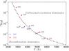 |
Fig. 19 Regimes of Mg I] λ4571 line formation in the [xMgI, T] plane. The values as a function of time for models 13C (blue crosses) and 13E (red circles) are also shown. The proximity to the dividing line between the two regimes means that both recombination and collisional excitation may contribute to the Mg I] λ4571 luminosity. |
5.7.2. Formation of Mg I λ1.504 μm and other magnesium lines
All other Mg I lines come from high lying states that are more difficult to populate by collisional excitation, and will form mainly through recombinations. Some empirical verification for this can be found by considering the relative line luminosities of Mg I λ1.183 μm and Mg I λ1.504 μm9. The Mg I λ1.183 μm line arises from a lower level than Mg I λ1.504 μm and has a larger collision strength relative to the ground state; consequently, collisional excitation should lead to a higher luminosity than in Mg I λ1.504 μm (both lines are allowed transitions to excited states and are thus de-excited by spontaneous radiative decay). The observed feature at 1.183 μm in SN 2011dh is, however, significantly weaker (not even clearly detected) than the 1.504 μm feature (Fig. 5), a situation which cannot be achieved in a collisional excitation scenario. The dominance of Mg I] λ4571 and Mg I λ1.504 μm in the observed spectra of these SNe is instead naturally explained in a recombination scenario, since these lines arise from triplet states which generally take most of the recombinations, whereas Mg I λ1.183 μm (and Mg I λ8807) arise from singlet states. The situation is analogous to the ratio of triplet to singlet recombination channels in He I, where ~3 / 4 of all recombinations go to the triplet ladder and ~1 / 4 to the singlet ladder (e.g. Benjamin et al. 1999). Another line in the triplet cascade that is predicted to be reasonably strong is Mg I λλ5167, 5173, 5184, which is blended with iron lines early on but may be seen at later times (Fig. A.3). Other lines include Mg I λλ7658, 7659, 7670 and Mg I λ1.577 μm, but they are both predicted as being too weak to be clearly discernable in the spectra.
5.7.3. Semi-analytical formulae for magnesium line luminosities
Having established that the nebular Mg I lines likely arise by recombination, with collisional excitation making some uncertain contribution to Mg I] λ4571, we can attempt an understanding of their luminosities. The critical density  (above which collisional de-excitation is important) for Mg I] λ4571 is found from equating the collisional and radiative de-excitation rates
  (5)where β4571 is the Sobolev escape probability. With A4571 = 217 s-1, T = 5000 K, gu = 9, and Υ4571 as previously specified, we get
 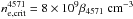 . In the models the optical depth of the Mg I] λ4571 line is of order unity in the nebular phase, so β4571 ≳ 0.1 and
  cm-3. This is higher than the electron density in the oxygen/magnesium zone in our models, so collisional de-excitation is unimportant and most populations of 3p(3P) will lead to emission of a 4571 Å photon. We can therefore write the luminosity of the Mg I] λ4571 line (assuming that recombination dominates and using the result that xMgI ≪ 1) as
 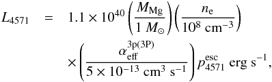 (6)where
  is the escape probability for the photon to pass through the SN ejecta without being absorbed by line blocking by other elements (or dust). The model calculations show that
  can be significantly smaller than unity far into the nebular phase (Sect. 6). For given values of MMg and , a higher electron density gives higher Mg I] λ4571 emissivity, so higher density of the magnesium clumps favours brighter Mg I] λ4571 (up to the limit when the critical density is reached or when xMgI ≪ 1 is no longer fulfilled).
The other distinct Mg I line observed is Mg I λ1.504 μm (Figs. 5 and 6). There is no strong blending of this line with any other lines in the models, and it has therefore a good diagnostic potential for the magnesium mass in the ejecta. Having a much higher critical density than Mg I] λ4571 (as it is an allowed transition to an excited lower level) and suffering no significant line blocking in the NIR, its luminosity should be given by 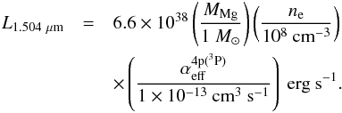 (7)In Appendix C we compute the effective recombination coefficient
  in both Case B and Case C at various temperatures. The physical conditions in the models at 200 days is close to Case C and T ~ 5000 K, for which
  cm3 s-1. We note that the Mg I λ1.488 μm recombination line will also blend with Mg I λ1.504 μm, but we find this contribution to be ≲10% and is ignored here.

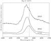 |
Fig. 20 Mg I] λ4571 feature in SN 2011dh. The line peak shows a blueshift of 1300 km s-1 at 200 days, which gradually diminishes and is smaller than 300 km s-1 at 415 days. |
Table 7 shows the measured luminosities of Mg I] λ4571 and Mg I λ1.504 μm in SN 2011dh, and the corresponding quantities neMMg derived from Eqs. (6) and (7). At 200 days the Mg I λ1.504 μm line gives a several times higher neMMg value than the Mg I] λ4571 line does, if is unity. Contribution by collisional excitation to Mg I λ4571 only makes this difference larger. This suggests that  , as the observed blueshift of the Mg I] λ4571 line also suggests (the peak of the line is blueshifted by 1300 km s-1 at 200 days, see Fig. 20). The Mg I λ1.504 μm line shows no blueshift, likely as there is much less line opacity in the NIR compared to the optical. If
  0.2 at 200 days, the derived neMMg values agree. As shown in Sect. 6, this is a typical value obtained when explicitly computing the line blocking opacity. The expected blueshift for a uniform sphere with a smooth radial opacity τ is ΔV/V = −1 + (ln(1 + τ)) /τ (Lucy et al. 1991), which has a value ΔV/V = −0.4 for τ = 1.5 (e-1.5 ~ 0.2). This matches the observed blueshift of Mg I] λ4571 (ΔV ~1300 km s-1) if V ~ 3300 km s-1, in good agreement with the observed line widths 10.
The blueshift of Mg I] λ4571 gradually disappears with time in SN 2011dh (Fig. 20) (as also obtained in the line blocking scenario, Sect. 6), reaching ΔV< 300 km s-1 at 415 days. This small blueshift requires τ< 0.2 from the Lucy formula, and so is close to unity and the neMMg values derived from the Mg I] λ4571 line listed in Table 7 at these epochs should be close to the true ones. Figure 21 shows how the Mg I] λ4571 line profile evolves in model 13E (chosen because it has distinct Mg lines and no dust) between 200 days (where there is significant line blocking) and 300 days (where most line blocking is gone). The total line profile is, as for the O I lines, affected in a complex way by both line blocking from the receding side and by blending with other emission lines.
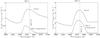 |
Fig. 21 Zoom-in on Mg I] λ4571 in model 13E at 200 days (left) and 300 days (right). The total flux and the contribution by Mg I are plotted. At 200 days there is significant line blocking of the red side of the Mg I emission (as well as a blend with some iron-group line emission). At 300 days both the line blocking and blending have abated. |
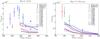 |
Fig. 22 Luminosity in Mg I] λ4571 (left) and Mg I λ1.504 μm (right) relative to the 56Co decay power in SN 1993J, SN 2008ax, and SN 2011dh, and in the models. The Mg I] λ4571 line is typically very blended in the models before 300 days, and so we do not plot the output of the line extraction algorithm before this time. |
5.7.4. The magnesium mass in SN 2011dh
The optical to NIR spectral coverage at 200 days of SN 2011dh allows us to combine the constraints from the oxygen and magnesium recombination lines to eliminate dependencies on the electron number density. From the oxygen recombination lines (Sect. 5.5) we have (estimating a 30% error)  cm-3, and from the Mg I λ1.504 μm line we have (estimating a similar error)
  cm-3. Combining these (assuming that the oxygen and magnesium recombination lines originate from the same regions, or that they have the same electron densities if not) we obtain a constraint
  M⊙. This range is plotted in Fig. 23. For a filling factor fO = 10-2, a magnesium mass of ~0.037 M⊙ is thus needed to reproduce the observed Mg I λ1.504 μm recombination line, whereas for fO = 0.1 a mass ~0.12 M⊙ is needed. A formal limit can be stated if we take the fO ≳ 10-2 constraint needed to make the [O I] λλ6300, 6364 lines optically thin early enough (Sect. 5.5), and fO< 0.07 from the fine-structure analysis in E14b, giving 0.020 M⊙<MMg< 0.14 M⊙. If we take the oxygen mass to have been constrained to 0.3−0.5 M⊙ (from the acceptable fits of the [O I] λλ6300, 6364 line luminosites, Fig. 15), the Mg/O mass ratio falls in the 0.04−0.5 range, or Mg/O = (0.3−4)(Mg / O)⊙. Thus, this analysis gives a Mg/O production ratio in SN 2011dh consistent with the solar ratio, but with relatively large error bars. The Mg / O ~ 1 / 2(Mg / O)⊙ production in the WH07 models lies at the lower end of the tolerance interval.
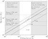 |
Fig. 23 Relationship between magnesium mass and oxygen zone filling factor derived from the oxygen and magnesium (Mg I λ1.504 μm) recombination lines in SN 2011dh. The solid line is the best estimate and the dashed lines show the error bars. The MMg-fO combinations of some models are shown as crosses. Also shown (as horizontal dotted lines) are the magnesium masses corresponding to a solar Mg/O ratio for the O masses for different MZAMS from WH07. The Mg/O ratio in the models is about half the solar Mg/O ratio. The regions ruled out by constraints from the [O I] λλ6300, 6364 lines are shaded grey. |
5.7.5. Magnesium lines in the model grid
Figure 22 shows Mg I] λ4571 and Mg I λ1.504 μm line luminosities in the observed spectra and in the models. Inspection of the model spectra shows that the Mg I] λ4571 line is often blended and/or has a strongly varying continuum (see e.g. Fig. 4). Before 300 days these effects are generally so large that the line luminosity extraction algorithm does not give any meaningful estimates for the line luminosity, and we therefore do not plot these. After 300 days these effects are less severe, but still sometimes significant in some of the models.
With these caveats in mind, the general trend from the Mg I] λ4571 and Mg I λ1.504 μm lines is an underproduction by the models. From the analysis above, there are likely two contributing factors to this; the factor of ~2 underproduction of magnesium in the WH07 models relative to the solar value, and a too low density (too large filling factor) assumed for the O/Ne/Mg zone in the models. The strong impact of the filling factor is illustrated by comparing model 13C (large filling factor, fO = 0.13 for the O/Ne/Mg zone) and model 13E (low filling factor, fO = 0.026) tracks. The Mg I λ1.504 μm line depends sensitively on density, and is a factor of 2−4 stronger in model 13E. The Mg mass is 0.044 M⊙ in these models. From the relationship between Mg mass and filling factor derived above, we would need fO = 0.014 to reproduce the Mg I λ1.504 μm line for that magnesium mass.
An even larger difference between 13C and 13E is seen with respect to Mg I] λ4571. Whereas 13E underproduces Mg I λ1.504 μm, it overproduces Mg I] 4571 at late times. Figure 19 shows that model 13E is in the regime of collisional pumping of Mg I] λ4571 at all times, whereas model 13C moves into the recombination regime after ~300 days. The growing difference in Mg I] λ4571 luminosities between 13C and 13E is thus due to the removal of collisional excitation contribution in the 13C model. In model 13E, Mg I] λ4571 does 5−20% of the cooling of the O/Ne/Mg zone throughout 100−500 days, whereas in 13C its cooling fraction is ~3% up to 300 days and then drops to to <1%.
5.8. Silicon lines
Figure A.3 (middle) shows the contribution by Si I to the model spectrum (higher ions produce negligible emission). The detectable lines are [Si I] λ1.099 μm, Si I λ1.200 μm11, and [Si I] λλ1.607, 1.646 μm. No detectable optical lines are predicted. The emission comes from the explosively synthesized silicon in the Si/S and the O/Si/S zones.
The [Si I] λ1.099 μm line blends with the red wing of [S I] λ1.082 μm + He I λ1.083 μm and is difficult to observationally disentangle. The Si I λ1.200 μm line appears to be seen in the observed spectra (Figs. 5 and 6). There is also a distinct line seen around 1.64 μm (Fig. 5), the model gives at this epoch about equal contributions from [Si I] λ1.646 μm and [Fe II] λ1.644 μm to this feature.
5.9. Sulphur lines
Figure A.3 (bottom) shows the contribution by S I and S II to the model spectrum (higher ions produce negligible emission). The sulphur lines arise from explosively made sulphur in the Si/S and O/Si/S zones (Fig. A.6). The only lines predicted to be strong are [S I] λλ1.082, 1.131 μm (the 1.082 μm line can be as strong as He I λ1.083 μm at late times and [S I] λ1.131 μm eventually becomes stronger than O I λ1.129 + λ1.130 μm). The S I λλ9213, 9228, 9237 feature causes some blending with O I λ9263 at early times. Note also [S II] λ1.032 μm12 which makes some blending with [Co II] λλ1.019, 1.025, 1.028 μm.
5.10. Calcium lines
Most of the calcium nucleosynthesis in SNe occurs in explosive oxygen burning, producing a Si/S zone that contains a small percent calcium by mass. In hydrogen-rich SNe this calcium is not visible as it is overwhelmed by emission from primordial calcium in the hydrogen envelope (Li & McCray 1993). Here, we find that in SN ejecta without such an envelope, the [Ca II] λλ7291, 7323 emission comes from the newly synthesized calcium. We find calcium not to be a prominent a cooler of the He (or H) envelope in the models here, as the radiation field is hard enough to ionize most of the calcium to Ca III in the nebular phase.
Figure 24 shows the observed and modelled [Ca II] λλ7291, 7323 and Ca II λλ8498, 8542, 8662 lines. In model 12C, the fraction of the cooling of the Si/S zone that is done by Ca II (and mainly [Ca II] λλ7291, 7323) is 100%, 83%, 67%, and 42% at 100, 200, 300, and 400 days, respectively. We are thus in a regime where the cooling of the Si/S zone is dominated by Ca II, and the Ca II luminosity is therefore not particularly sensitive to the Ca II mass, but rather depends on the amount of gamma-ray and positron energy being reprocessed by the Si/S zone, which in turn depends on the mass of the Si/S zone. The satisfactory agreement between observed and modelled Ca II lines (Fig. 24) thus supports the mass of the explosive oxygen burning ashes in the models used; ~0.1 M⊙.
We find that most of the Ca II λλ8498, 8542, 8662 emission does not originate from the calcium in the Si/S zone; this zone is generally too cool (T< 3000 K after 200 days) to excite the 4p(2P) parent state. The IR lines instead arise primarily by fluorescence following absorption in the HK lines by Ca II in the Fe/Co/He clumps. The radiative de-excitation rate for the return transition in HK is  s-1, and for the IR channel
  s-1. The optical depth in the IR channel is always smaller than in the HK channel, as the IR transitions go to the excited state 3d(2D) which always has a much smaller population than the ground state. Since also βHK ≪ 1 in the Fe/Co/He zone at all times, the result it that
  , and most HK absorptions in the Fe/Co/Ni zone are followed by fluorescence in the IR lines. In the helium and hydrogen envelopes, on the other hand, the density is low enough that significant de-excitation occurs back in the HK lines.
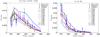 |
Fig. 24 Left: luminosity in [Ca II] λλ7291, 7323 relative to the 56Co decay power in SN 1993J, SN 2008ax, SN 2011dh, and in the models. Right: same for the Ca II IR lines. |
5.11. Titanium lines
Figure A.4 shows the contribution by titanium to the spectrum, which can be seen to be significant at early times. Titanium is an effective line blocking agent, and provides much of the quasi-continuum through scattering and fluorescence at early times.
5.12. Iron lines
Figure A.4 (bottom panel) shows the contribution by Fe I, Fe II, and Fe III to the model spectrum. These components are strong at all times. The iron lines arise from both cooling and recombination of the iron from decayed 56Co, but also from scattering in this component and from primordial iron in the rest of the nebula.
The most distinct iron lines emerging in the model are [Fe II] λ7155, [Fe II] λ1.257 μm, a [Fe II] complex between 1.27−1.32 μm, [Fe II] λ1.534 μm, [Fe II] λ1.644 μm, and [Fe II] λλ1.801, 1.810 μm. Most of these lines appear to be present in the spectra of SN 2011dh (Figs. 4 and 5).
The [Fe II] λ7155 line has an excitation temperature of 22 800 K whereas the [Fe II] λ1.257 μm line has an excitation temperature of 11 500 K, so their ratio is temperature sensitive. Both lines are optically thin from 100 days in model 12C. In the models, the 4s(a4D) level (giving the [Fe II] λ1.257 μm line) is in LTE for a few hundred days, but 3d7(a2G) (giving the [Fe II] λ7155 line) is in NLTE already at 100 days. In the LTE and optically thin limit 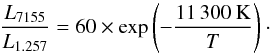 (8)The [Fe II] λ7155 line is quite heavily blended with [Ca II] λλ7291, 7323 on the red side and He I λ7065 on the blue side, and its flux is therefore hard to determine. At 100 days it is not visible in SN 2011dh. At 200 days we estimate the [Fe II] λ7155 luminosity to L7155 ≈ 4 × 1037 erg s-1. The [Fe II] λ1.257 μm line is noisy but we estimate L1.257 ≈ 3 × 1037 erg s-1, giving a ratio of 1.3. The LTE temperature is TLTE = 3000 K. The model temperature in the Fe/Co/He zone is 5000 K at 200 days. The deviation from LTE for level 3d7(a2G) is about a factor of two in the model at this time, which means that the LTE assumption gives a somewhat too low temperature. Using a departure coefficient of 0.5 gives a temperature of 3600 K.
For a given temperature, the Fe II mass can be estimated from 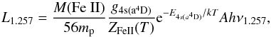 (9)which gives M(Fe II) = 0.033 M⊙ for T = 3000 K and M(Fe II) = 0.090 M⊙ for T = 5000 K. Assuming that M(Fe) ≈ M(Fe II) and that this iron comes from 56Ni, the initial 56Ni mass is M(56Ni) = 0.19 M⊙ for T = 3000 K and 0.051 M⊙ for T = 5000 K. The iron lines are thus consistent with approximately 0.1 M⊙56Ni being synthesized in the SN explosion, although uncertainty in the line luminosity measurements as well as temperature make it difficult to determine the 56Ni mass as accurately as is possible from the light curve phase (Bersten et al. 2012, E14b).
5.13. Cobalt lines
Figure A.5 (top panel) shows the contribution by Co II to the spectrum (contributions by other cobalt ions are negligible). The models predict strong [Co II] λλ9336, 9343, [Co II] λλ1.019, 1.025, 1.028 μm, and [Co II] λ1.547 μm at early times, arising from the radioactive 56Co. At later times most of the 56Co has decayed and the lines become weaker. All lines suffer some blending; [Co II] λλ9336, 9343 with O I λ9263, [Co II] λλ1.019, 1.025, 1.028 μm with [S II] λ1.032 μm, and [Co II] λ1.547 μm with [Fe II] λ1.534 μm. The [Co II] λλ1.019, 1.025, 1.028 μm triplet is the strongest predicted cobalt feature and has the least blending of these three, it is therefore the most promising diagnostic of the 56Co mass.
The early spectra of SN 2011dh are consistent with the presence of these lines (Figs. 4 and 5). The modelled [Co II] λλ1.019, 1.025, 1.028 μm line is in reasonable agreement with the observed lines in SN 2011dh and SN 2008ax (Figs. 5 and 6). These lines are, at 200 days, optically thin but in NLTE in the models.
5.14. Nickel lines
Figure A.5 (middle panel) shows the contribution by Ni II to the spectrum (emission from other nickel ions is negligible). The radioactive nickel quickly decays and is not present in large enough quantities to be visible in the nebular phase. However, some stable nickel (mainly 58Ni) is created alongside the 56Ni, which gives rise to [Ni II] λλ7378, 7411 emission. This doublet will in general blend with the red wing of [Ca II] λλ7291, 7323.
Figure A.5 shows that identification of 58Ni may also be done by [Ni II] λ1.939 μm, which arises from the same upper level as [Ni II] λλ7378, 7411. The day 202 spectrum of SN 2011dh shows an emission line at this wavelength (Fig. 5).
5.15. Other lines
Figure A.5 (lower panel) shows the contribution to the spectrum by all other elements not covered in previous sections; these are Ne, Al, Ar, Sc, V, Cr, and Mn. It is clear that emission and scattering by these elements make up a relatively minor part of the spectrum, and that the individual elements analysed in previous sections together account for most of the optical/NIR flux.
6. Radiative transfer effects on line profiles
The strong velocity gradients in SN ejecta allow lines to collectively provide significant opacity as photons redshift through an extensive wavelength range with respect to the comoving frame as they traverse the ejecta. The collective opacity is referred to as line blocking, and can be significant long after the ejecta have become optically thin in the continuum. This line blocking opacity is especially important in the UV and at short optical wavelengths, where thousands of iron-group lines reside.
Figure 25 shows that the observed line profiles of both [O I] λ5577 and [O I] λλ6300, 6364 evolve quite significantly between 100 and 200 days in SN 2011dh. At 100 days the peaks of the lines are both blueshifted by ~1500 km s-1, but at 200 days the blueshift is much less. A plausible interpretation is that the early blueshifts arise as a result of line blocking, which preferentially absorbs emission from the receding side of the ejecta, and is an effect that diminishes with time. We note that the Na I-D line is not noticeably affected, as it is mainly formed by scattering in the envelope (giving a P-Cygni like profile) and experiences little transfer through the metal-rich core.
This idea is supported by the radiative transfer simulations performed here which give significant line blocking at optical wavelengths at 100 days. In Fig. 26 we show the model spectra (13E) at 100 and 200 days zoomed in on the oxygen lines. We obtain significant blueshifts of [O I] λ5577 and [O I] λλ6300, 6364 at 100 days. At 200 days the line blocking has decreased and the model gives more symmetric lines profiles. The evolution therefore matches the observed one in SN 2011dh.
A similar effect is seen in most other stripped envelope SNe with respect to Mg I] λ4571, [O I] λ5577, and [O I] λλ6300, 6364 (Taubenberger et al. 2009, M10). In SN 1993J and SN 2008ax, the [O I] λ5577 line also showed a blueshifted peak at early times (~2000 km s-1, Spyromilio 1994, M10). In SN 2008ax the blueshift slowly diminished with time (M10), but in SN 1993J there was no discernible reduction until the line disappeared (Spyromilio 1994).
In cases where line asymmetries persist for several hundred days, ejecta asymmetries are often invoked. The consistency of blueshifts (only unshifted or blueshifted cases were observed for Mg I] λ4571, [O I] λ5577, and [O I] λλ6300, 6364 in the sample of stripped-envelope SNe presented by M10) makes both asymmetries and line blending unlikely explanations. The only scenario that can explain such systematic line shifts towards the blue is selective absorption of emission from the receding side of the SN, which as discussed above (see also below) is seen when the radiative transfer problem is solved. The evolution of the line blocking depends on the density of the homologously expanding ejecta. One possible scenario is that SNe which show slow line profile changes (such as SN 1993J) have higher density ejecta and therefore maintain the line-blocking opacity for a longer time.
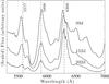 |
Fig. 25 Zoom-in on the [O I] λ5577, Na I λλ5890, 5896 and [O I] λλ6300, 6364 lines in SN2011dh at 99, 152, and 202 days. Both oxygen lines show blueshifted line profiles at 99 days, but the peaks then gradually move towards zero velocity. The Na I D lines show no blueshift as they mainly arise from envelope scattering (giving a P-Cygni like profile) rather than from the self-absorbing core. |
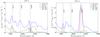 |
Fig. 26 Model spectra (model 13E, chosen for not having any dust to influence the line profiles) at 100 days (left) and 200 days (right), showing total flux (blue) and the contributions by O I (red), Si II (black), Fe II (green), and Sc II (cyan). Distinct blueshifts of [O I] λ5577 and [O I] λλ6300, 6364 occur in the model at 100 days. At 200 days these effects are less severe and the model gives more symmetric line profiles. |
Figure 27 shows, for model 13G at 100 and 200 days, the integrated line optical depth between λ and λ × (1 + Vcore/c) (Vcore = 3500 km s-1) multiplied by zone filling factor fi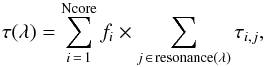 (10)where a line j belongs to the resonance set if its wavelength is between λ and λ × (1 + Vcore/c). This quantity gives some information about the line blocking optical depth of the SN core, telling us the wavelength variation, and the components can also be analyzed to show the relative importance of the different zones. The figure shows that both the iron-group element zones (Fe/Co/He + Si/S) and the oxygen-rich zones (O/Si/S, O/Ne/Mg, O/C) provide significant optical depth, with the iron-group zones providing more optical depth at shorter wavelengths and the oxygen-rich zones providing more at longer wavelengths.
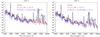 |
Fig. 27 Integrated optical depth times filling factor (see Eq. (10)) in model 13G, at 100 days (left) and 200 days (right). Also plotted is the contribution by the iron-sulphur clumps (red) and the oxygen clumps (blue). |
Figure 28 shows the escape probability for a photon emitted at the centre of the core to reach the surface of the core without being absorbed by a line, computed as 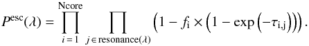 (11)The figure demonstrates that below ~6000 Å, the ejecta are opaque for hundreds of days because of line blocking. At longer wavelengths the core is mostly transparent after 200 days, apart from some individual lines such as the Ca II NIR triplet. The emergent optical/NIR spectrum still depends, however, on the radiative transport through the influence of absorption by λ ≲ 6000 Å photons on temperature, ionization, and excitation (including fluorescence).
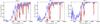 |
Fig. 28 Escape probability for a photon to pass through 3500 km s-1 of core material (model 13G), at 100 (left), 200 (middle), and 400 (right) days (black). Also plotted are escape probabilities with respect to passage through the Fe/Co/He and Si/S clumps (red) and the O/Si/S, O/Ne/Mg, and O/C clumps (blue). |
Figure 29 shows the time evolution of the escape probability pesc(λ) at 4571 and 6300 Å. There is, as expected, a continuous increase towards unity as the optical depths decrease with time.
7. Influence of model parameters
7.1. Progenitor mass
The model combinations that differ only in the progenitor mass are 12C, 13G, and 17A. Figure 30 shows the optical/NIR spectra of these models at 300 days. The overall brightness increases with MZAMS because of the higher gamma-ray deposition in higher-mass ejecta. As the physical conditions change, different spectral lines will brighten by different amounts, and some may decrease.
As illustrated here (and in Fig. 15) one of the key differences between these models is the [O I] λλ6300, 6364 luminosity; it is a factor of 4−5 higher for ejecta from a 17 M⊙ progenitor compared to a 12 M⊙ progenitor. The fact that this line grows brighter by a much larger factor than the increase in global energy deposition (which increases by a factor of ~2 from MZAMS = 12 to MZAMS = 17 at 300 days) makes it an excellent tool for estimating the progenitor mass. The [O I] λ5577 line, which is only visible at earlier times, has a similar dependency on the progenitor mass (Fig. 17), and the [O I] λ5577/[O I] λλ6300, 6364 ratio is little affected. This can be understood from the fact that we are in the regime where the ejecta are optically thin to the gamma rays, and the energy deposition per unit mass (which governs the temperature) is therefore roughly independent of the ejecta mass. Indeed, we find in the 12C, 13G, and 17A models at 300 days an O/Ne/Mg zone temperature varying by less than 100 K.
Mg I] λ4571 also becomes stronger for higher progenitor masses (Fig. 30). As the O/Ne/Mg zone density is similar in the three models, the neutral fraction of magnesium becomes similar, leading to a small variation in the relative contributions by collisional excitation and recombination to the Mg I] λ4571 emissivity (Sect. 5.7). The Mg I λ1.504 μm line is weak at 300 days and difficult to discern, but is also stronger for higher mass progenitor models.
As discussed in Sect. 5.6, the Na I D lines have contributions from both a scattering component (mainly from the helium envelope) and a cooling/recombination component from the synthesized sodium. Figure 30 shows that a distinct component from the synthesized sodium is produced in the 17 M⊙ ejecta, clearly distinguishable from the scattering-dominated component seen at lower masses.
The [Ca II] λ7291, 7323 lines also increase in strength with progenitor mass, although quite weakly (see also Fig. 24). As the [Ca II] λλ7291, 7323 lines dominate the cooling of the oxygen burning ashes (the Si/S zone), their luminosities are mainly dependent on the mass of this zone. An important difference to the oxygen lines is that the oxygen burning is explosive and depends not only on the progenitor but also on the explosion properties. The calcium lines are therefore less directly linked to the progenitor mass than the oxygen lines are. With the assumed explosion properties in the WH07 models, the Si/S zone mass varies between 0.06 to 0.11 M⊙ over the MZAMS = 12−17 M⊙ range, giving a factor of ~2 variation in the [Ca II] λλ7293, 7323 lines. In the 17 M⊙ model there is, however, also some contribution to [Ca II] λλ7291, 7323 from the O/Ne/Mg zone.
Except for t ≲ 200d, the Ca II IR triplet does not arise from the synthesized calcium but from fluorescence following Ca II HK absorption in other zones (Sect. 5.10). In the models here, [C I] λ8727 (cooling of the O/C zone) is stronger than the Ca II IR triplet at 300 days. Higher MZAMS give brighter emission in both the Ca II IR triplet and in [C I] λ8727.
In the NIR, the largest differences are seen for [S I] λλ1.082, 1.131 μm, and [Si I] λλ1.607, 1.646 μm (Fig. 30). The strong sulphur lines in the 17 M⊙ model arise from the O/Si/S zone, which has a higher sulphur content (32%) than in the lower-mass ejecta (4%).
7.2. Mixing
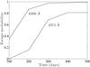 |
Fig. 29 Core escape probability with respect to line blocking (from Eq. (11)) at 4571 Å and 6300 Å as a function of time, for model 13G. |
Figure 31 compares spectra of model 13A (medium mixing) and 13C (strong mixing) at 200 days. As a first order effect, more outmixed 56Ni gives a lower total gamma-ray deposition and therefore dimmer nebular spectra. Very temperature-sensitive lines, such as [O I] λ5577, show the strongest drops when the deposition decreases, but also lines such as [O I] λλ6300, 6364 and O I λ7774 lose significant luminosity. The lines from the Fe/Co/He zone become both dimmer (because of the lower energy deposition) and less distinct as the line profiles obtain broader bases and less pronounced peaks.
The way these models are constructed, changing the mixing also changes zone densities, and the detailed reasons for various line luminosity variations is not possible to deduce in any straightforward manner. Since different zones have different opacities (because of their differing metal content), the mixing also effects the radiative transport and the line blocking.
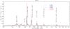 |
Fig. 30 Optical/NIR spectrum at 300 days for different progenitor masses (models 12C, 13G, and 17A). The most sensitive (bright) lines are marked. |
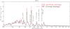 |
Fig. 31 A comparison of models with medium mixing (13A, red dashed) and strong mixing (13C, black solid) at 200 days. The most sensitive (bright) lines are marked. |
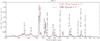 |
Fig. 32 A comparison of models with non-locally (13A, red dashed) and locally (13B, black solid) absorbed positrons, at 400 days. The most sensitive (bright) lines are marked. |
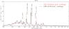 |
Fig. 33 A comparison of models without (12C, red dashed) and with (12D, black solid) molecular cooling of the O/Si/S and O/C zones, at 200 days. The most sensitive (bright) lines are marked. |
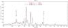 |
Fig. 34 A comparison of models with low (13C) and high (13E) contrast factor χ, at 300 days. The most sensitive (bright) lines are marked. |
7.3. Positron trapping
We can distinguish three different phases in models where the positrons are free to stream into adjacent zones; a first phase where the energy deposition in each zone is little changed compared to an on-the-spot treatment, a second phase where the energy deposition in the 56Ni-containing clumps decreases significantly if positrons are allowed to stream out of them, and a third phase where deposition in each ejecta zone varies significantly with the positron treatment (typically when the total positron deposition is comparable to (or exceeds) the total gamma-ray deposition).
Looking at models 13A and 13B, and taking a deposition difference by 30% as the criterium for “significant difference”, we find that the first phase spans ~0−200 days, the second phase ~200−400 days, and the third phase ≳400 days. During the second phase the spectrum will show moderate changes, only related to changes in Fe/Co/Ni lines, whereas during the third phase significant variation in line emission from other zones may also occur.
To study the influence of the positron treatment, we compare models 13A (non-local e+ absorption) and 13B (local e+ absorption). Figure 32 compares these models at 400 days. The late-time deposition of positron energy in the oxygen clumps gives model 13A an [O I] λλ6300, 6364 doublet that does not fall off in time as observed, but is too bright after 200 days (see also Fig. 15). In all three observed SNe, Lnorm(t) for [O I] λλ6300, 6364 peaks at around 200 days and shows a decline between 200 and 400 days, which is reproduced by 13B (and most other models with local e+ absorption), but not by 13A (and most other models with non-local e+ absorption). A caveat here, however, is that if molecular cooling is strongly time-dependent and increases significantly after 200 days, it could lower these curves at late times, while changing them little at earlier times. Without a detailed calculation of the molecular cooling (which would need the incorporation of molecular networks such as those described in Cherchneff & Dwek 2009), it is therefore difficult to draw firm conclusions regarding the positrons from the late-time behaviour of [O I] λλ6300, 6364.
The magnesium lines also become brighter with non-local positron deposition (Fig. 22), as the higher electron density produced by the higher ionization level gives stronger recombination.
As the Fe/Co/He clumps receive less energy input in non-local models, they are cooler and emit weaker lines, a difference that begins in phase two and continuously grows stronger with time. As Fig. 32 shows, many iron and cobalt lines in the NIR differ significantly between the models at late times. Unfortunately, at the time of the last NIR spectrum in our dataset (200 days for SN 2011dh), the difference is not yet large enough (about 10%) to differentiate between the scenarios. In the optical, however, [Fe II] λ7155 is observed at late times. With local positron absorption, this line is significantly stronger than with non-local absorption. The observed line at late times in SN 2011dh appears to fit the non-local scenario better (Figs. 4 and 32), although the vicinity to the strong [Ca II] doublet complicates the analysis. At 400 days, the non-local model produces no detectable line at all, whereas the local model produces one that is several times too strong, so neither model is fully satisfactory.
Putting all the comparisons with data together, we thus find no model that is fully satisfactory in terms of the positron treatment. It appears that wherever the positrons are taken to deposit their energy, they produce too strong emission lines; too strong [O I] λλ6300, 6364 if allowed to stream into the oxygen zones, and too strong [Fe II] λ7155 if trapped locally in the iron clumps. The situation is reminiscent of modelling of the spectrum of SN 1987A at an age of eight years (Jerkstrand et al. 2011), where similar results were obtained (but here either [O I] λλ6300, 6364 or [Fe II] 26 μm were overproduced instead of [O I] λλ6300, 6364 or [Fe II] λ7155). One possible solution could be significant reemission by dust or molecules from whatever zones the positrons deposit their energy in. This is an attractive scenario given the strong MIR emission observed from SN 2011dh at late times (E14b).
7.4. Molecular cooling
Models with molecular cooling have their atomic cooling emission from the O/Si/S and O/C zones damped out. The impact of this can be studied by comparing models 12C (no molecular cooling) and 12D (full molecular cooling of O/Si/S and O/C zones). Figure 33 compares these models at 200 days. The impact is significant on [O I] λ5577, [O I] λλ6300, 6364, [C I] λ8727 (a strong cooler of the O/C zone in the absence of CO cooling), [Ca II] λλ7291, 7323, and Ca II IR (strong coolers of the O/Si/S zone in the absence of SiO cooling (Ca II IR only for t ≲ 200d)). The biggest difference between the models at 200 days is the Ca II IR + [C I] λ8727 blend. Compared to SN 2011dh, this blend is better reproduced in models with no molecular cooling than those with complete molecular cooling (as seen by comparing Fig. 4 (second panel) and Fig. 33), suggesting that CO and SiO cooling play a minor role at this time.
The impact of the molecular cooling depends on the progenitor mass, as the relative masses of the O/Si/S, O/Ne/Mg, and O/C zones vary significantly with progenitor mass. For instance, at MZAMS = 12 M⊙, these zone masses are 0.13, 0.14, and 0.16 M⊙, whereas at MZAMS = 18 M⊙ they are 0.27, 1.2, and 0.58 M⊙. Since the O/Ne/Mg zone is much more massive than the others in high-mass progenitors, the impact of molecular cooling on the oxygen lines is smaller, since molecules form mainly in the O/Si/S and O/C zones (Liu & Dalgarno 1995). The conclusions regarding upper limits to the progenitor masses based on the [O I] λλ6300, 6364 lines are therefore robust with respect to uncertainties in molecular cooling. A 17 M⊙ model with molecular cooling has only ~1/3 weaker [O I] λ6300, 6364 emission lines compared to a model without molecular cooling, and still overproduces the observed [O I] λλ6300, 6364 emission in all three SNe studied here. For low-mass progenitors, on the other hand, ~2/3 of the oxygen mass is in the O/Si/S and O/C layers, and the oxygen emission is more sensitive to molecular cooling.
7.5. Dust
There are two main influences of dust on the optical/NIR spectrum; the dust suppresses the flux levels (by approximately a factor exp(−τdust)), and it leads to line profile distortions due to the preferential absorption of emission from the receding side of the ejecta. In a situation of a uniform distribution of line emission and dust absorption, the peaks are blueshifted by an amount given by (Lucy et al. 1991) ΔV = Vcore × [(ln(1 + τ)) /τ − 1] which is ~400 km s-1 for Vcore = 3500 km s-1 and τ = 0.25 (the dust optical depth used in the dust models). This distortion further complicates the interpretation of the observed line profiles, as the mechanism is similar to the one of line opacity discussed in Sect. 5.5. Whereas the line blocking decreases with time (although the optical depth of some particular lines may temporarily increase because of changes in ionization and temperature), dust blocking can both increase and decrease with time, depending on how the dust formation process evolves. If the dust is optically thin, an increase of its blocking may occur if the dust formation occurs faster than the t-2 decline of the column densities. If the dust is optically thick, the blocking will depend on how many optically thick clumps are present at any given time, which could also both increase and decrease with time.
There will also be second order effects from changes in temperature and ionization caused by the suppression of the internal radiation field, but the dominance of radioactivity for the total energy deposition in the various zones means that these effects are quite small, at least for the moderate dust optical depths (τ = 0.25) explored here.
7.6. Density contrast factor χ
The influence of the core zone densities was discussed in some detail in Sects. 5.5 and 5.7 regarding oxygen and magnesium lines. To recap, the influence on the [O I] λλ6300, 6364 cooling lines is relatively small because oxygen is dominantly neutral over the whole density range analysed (χ = 30−210), it reemits a large fraction of the thermal energy deposited in the oxygen clumps, and the fraction of the non-thermal energy going into heating depends only weakly on the density (Kozma & Fransson 1992). That this is the case can be seen by comparing the strengths of the [O I] λλ6300, 6364 lines between models 13C and 13E, which differ only in contrast factor χ; 13C has a low χ (low oxygen zone density) and 13E has high χ (high oxygen zone density). Figure 34 shows that the [O I] λλ6300, 6364 lines are ~20% brighter in the high-density model at 300 days, and Fig. 15 shows that this holds true between 100−350 days. After that time, the low-density model becomes brighter.
The charge transfer quenching of oxygen recombination lines that can occur at high densities and low ionization levels (Sect. 5.5) is clearly illustrated in Fig. 34; the high-density model 13E has very weak oxygen recombination lines. For minor species like magnesium and sodium, higher density instead leads to stronger recombination lines. The situation for these elements is that the radiation field is strong enough to keep them fully ionized over a broad range of densities, rather than becoming more neutral at higher densities as happens with oxygen (a process which is accelerated by charge transfer). The recombination emission is then proportional to the electron density (see Sect. 5.7), which grows approximately with the square root of the density.
As is clear from Fig. 34, there are no other major changes due to the χ factor. In particular, one should note that the Fe/Co/He zone density only changes by 30% as χ goes from 30 to 210, as in both scenarios it takes up a large fraction of the core (filling factors 0.59 and 0.78 in 13C and 13E, respectively).
8. Summary and conclusions
We have investigated optical/NIR line formation processes in Type IIb SNe from 100 to 500 days post-explosion using NLTE radiative transfer simulations, and compared these models with the three best observed Type IIb SNe to-date; SN 1993J, SN 2008ax, and SN 2011dh.
We find the principal components of the model spectra to be cooling and recombination emission from hydrostatic hydrogen burning ashes (He I λ1.083 μm, He I λ2.058 μm, [N II] λλ6548, 6583), helium burning ashes ([C I] λ8727, [C I] λλ9824, 9850, [O I] λλ6300, 6364), carbon burning ashes ([O I] λ5577, [O I] λλ6300, 6364, O I λ7774, O I λ9263, O I λ1.129 μm + λ1.130 μm, O I λ1.316 μm, Mg I] λ4571, Mg I λ1.504 μm, Na I-D), and from explosive burning ashes ([Si I] λ1.099 μm, [Si I] λ1.200 μm, [Si I] λλ1.607, 1.646 μm, [S I] λλ1.082, 1.311 μm, [S II] λ1.032 μm, [Ca II] λλ7291, 7323, Ca II IR, [Fe II] λ7155, [Fe II] λ1.257 μm, [Fe II] λ1.534 μm, [Fe II] λλ1.801, 1.810 μm, [Co II] λλ9336, 9343, [Co II] λλ1.019, 1.025, 1.028 μm and [Ni II] λλ7378, 7411). These strong emission lines sit atop a quasi-continuum of weaker lines, mainly from iron and titanium, arising by emission as well as scattering/fluorescence from the iron clumps and from the helium envelope. This fluorescent component also produces much of the Ca II NIR triplet, especially after 200 days.
The outer parts of the helium envelope are rich in nitrogen from CNO burning, and this leads to strong [N II] λλ6548, 6583 emission. In the models this emission dominates over the Hα emission by one to two orders of magnitude after ~150 days. We find that there is too little hydrogen in Type IIb SNe to produce any detectable Hα, or any other emission lines, after 150 days (and this means that the models computed here are applicable to Type Ib SNe as well for t> 150 days). Although interaction-powered Hα was clearly present in the spectrum of SN 1993J at late times, our models closely reproduce the evolution of the observed feature around 6650 Å in SN 2008ax and SN 2011dh with [N II] λλ6548, 6583 dominating the emission.
Oxygen and magnesium lines are particularly distinct in Type IIb (as well as in Type Ib/c) SNe, and we therefore make a thorough investigation of the diagnostic use of these lines. The cooling lines of [O I] λλ6300, 6364 (as well as [O I] λ5577) are suitable for estimating the helium core mass of the progenitor, and ejecta models from helium cores MHe−core = 3−5 M⊙ (MZAMS = 12−16 M⊙, oxygen masses 0.3−0.9 M⊙) satisfactorily reproduce these collisionally excited oxygen lines in the three SNe studied here. Although the link between progenitor main-sequence mass and oxygen production depends on the stellar evolution model used, the variation between published models for a given ZAMS mass is at most a factor of 2 (see discussion in Jerkstrand et al. 2014) and this uncertainty would still not allow for the high masses (MZAMS ≳ 25 M⊙) needed to produce hydrogen envelope stripping by single star winds. Nucleosynthesis analysis thus supports a low-to-moderate mass origin for Type IIb SNe, and by implication binary progenitor systems.
Magnesium has two distinct emission lines, Mg I] λ4571 and Mg I λ1.504 μm. We find that Mg I] 4571 has contributions from both thermal collisional excitation and recombination, whereas Mg I λ1.504 μm is a recombination line. Based on the regime of physical conditions that the model calculations give, semi-analytical formulae are derived that allow a determination of the magnesium mass from the combined use of magnesium (Mg I λ1.504 μm) and oxygen (O I λ7774, O I λ9263, O I λ1.129 μm + λ1.130 μm, O I λ1.316 μm ) recombination lines. For SN 2011dh, we use this method to determine a magnesium mass of 0.020−0.14 M⊙, which is consistent with a solar Mg/O production ratio.
The most distinct helium lines are He I λ1.083 μm and He I λ2.058 μm, although He I λ1.083 has some blending with [S I] λ1.082 μm and [Si I] λ1.099 μm. We find that the ejecta models investigated here give good reproductions of the NIR helium lines in SN 2008ax and SN 2011dh, indicating ejected helium masses of about 1 M⊙. These helium lines are mainly formed by recombination, although at late times cooling and non-thermal excitations contribute to He I λ1.083 μm and He I λ2.058 μm, respectively. Scattering also contributes, as these lines (and also He I λ5016) stay optically thick for several hundred days.
The [Ca II] λλ7293, 7323 lines constrain the mass of the oxygen burning layer, and we find a good fit with the Si/S zone masses in the models used here, which are around 0.1 M⊙.
Even as steady-state conditions for the radiative transport set in after 50−100 days in stripped envelope ejecta (i.e. the timescale for the radiative transport is shorter than the dynamic and radioactive timescales), we show here how the large velocity gradients lead to significant line blocking effects for several hundred days. These radiative transfer effects lead to a complete reprocessing of emission blueward of ~6000 Å, and blueshifted emission line profiles for optical lines from the core such as Mg I] λ4571 and [O I] λλ6300, 6364. The blueshift gradually diminishes with time as the densities decrease, matching the observed evolution in SN 2011dh as well as in samples of stripped-envelope SNe (Taubenberger et al. 2009, M10).
For the Type IIb class, observations and modelling of progenitor luminosities, diffusion phase light curves, and nebular phase spectra are at this point in relatively satisfactory agreement with each other regarding at least some physical parameters. Of the three best observed events, at least two (SN 1993J and SN 2011dh) had yellow supergiant progenitors (Aldering et al. 1994; Maund et al. 2011), light curves that were fit with ejecta masses of 2−3 M⊙ (Woosley et al. 1994; Bersten et al. 2012, E14b), and nucleosynthesis (in particular oxygen) in agreement with MZAMS = 12−16 M⊙ progenitors (Houck & Fransson 1996; Shivvers et al. 2013, this paper). Binary stellar evolution codes can explain the progenitor structures by Roche lobe overflow (e.g. Benvenuto et al. 2013), although attempts to reproduce the observed rates have so far not been successful (Claeys et al. 2011). The search for a binary companion to SN 2011dh will provide a crucial test for the binary progenitor hypothesis, as it did for SN 1993J (Maund et al. 2004).
Online material
Appendix A: Element and zone contributions
Figures A.1 to A.8 show the contribution by all major elements and zones to the emergent spectra of model 13G at 100, 300, and 500 days. These figures allow an overview of the various contributions and can be used for guidance in line identifications in other SNe.
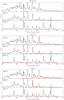 |
Fig. A.1 Top: contribution by H I lines (red) to the spectrum in model 13G (black), at 100, 300, and 500 days. Middle: same for He I. Bottom: same for C I. |
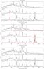 |
Fig. A.3 Top: same as Fig. A.1 for Mg I (red) and Mg II (green). Middle: same for Si I. Bottom: same for S I (red) and S II (green). |
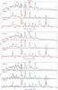 |
Fig. A.4 Top: same as Fig. A.1 for Ca II. Middle: same for Ti II. Bottom: same for Fe I (red), Fe II (green), and Fe III (blue). |
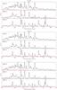 |
Fig. A.5 Top: same as Fig. A.1 for Co II. Middle: same for Ni II. Bottom: same for all remaining elements (Ne, Al, Ar, Sc, V, Cr, Mn). |
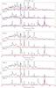 |
Fig. A.6 Top: same as Fig. A.1 for the Fe/Co/He zone (red is the total contribution, blue is the contribution by the core component). Middle: same for the Si/S zone. Bottom: same for the O/Si/S zone. |
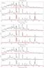 |
Fig. A.7 Top: same as Fig. A.1 for the O/Ne/Mg zone. Middle: same for the O/C zone. Bottom: same for the He/C zone. |
Appendix B: Code updates
Appendix B.1: Atomic data
-
Mg I. Total radiative recombination rate updated, now from Badnell (2006). The dielectronic recombination rate is from Nussbaumer & Storey (1986). We compute specific recombination rates by applying the Milne relations to the TOPBASE photoionization cross sections (Cunto et al. 1993) for the first 30 (up to 3s6d(1D)) multiplets. For higher states, allocation of the remaining part of the total rate occurs in proportion to statistical weights, as described in Jerkstrand et al. (2011). There are some issues with applying the Milne relations to the TOPBASE bound-free cross sections; these include ionization to excited states, whereas we need the cross section for ionization to the ground state. The first excited state in Mg II has, however, an excitation energy of 4.42 eV, so for the moderate temperatures (T ≲ 104 K) of interest here, the contribution by the cross section at these high electron energies is small, and it should be a good approximation to use the full TOPBASE cross sections. Another complication is that the ionization thresholds given by TOPBASE are often somewhat offset from their correct values. One may choose to renormalize all energies to the correct threshold, here we have not done so (so we simply ignore any listed cross sections at energies below the ionization edge). We solve for statistical equilibrium for a 112 level atom (up to 15f(3F)). For higher levels our dataset on radiative transitions is incomplete and using a larger atomic model would therefore give a biased recombination cascade.
-
Na I. Total recombination rate from Verner & Ferland (1996). Specific recombination rates for first 16 terms (up to 6d(2D)) computed from TOPBASE photoionization cross sections (same as in Jerkstrand et al. (2011) but not fully clarified there). The collision strengths are from Trail et al. (1994) for the Na I D line, and from Park (1971) for the other transitions. The Trail et al. (1994) value is in good agreement with the recent calculation by Gao et al. (2010).
-
O I. Specific recombination rates from Nahar (1999) implemented for the first 26 terms (up to 5f(3F)).
-
S I. Forbidden line A-values updated with values from Froese Fischer et al. (2006) (via NIST).
-
Others. Added Ni III, with energy levels from Sugar & Corliss (1985) (up to 3d8(1G)) (via NIST), A-values from Garstang (1958) (via NIST), collision strengths (from ground multiplet only) from Bautista (2001). Added dielectronic recombination rates for Si I, Si II, S I, Ca I, Fe I, and Ni I (Shull & van Steenberg 1982). Added forbidden lines for Fe III, Co III, Al I, Al II, Ti I, Ti II, Ti III, Cr I, Cr II, Mn II, V I, V II, Sc I, Sc II (kurucz.harvard.edu). Added Fe III collision strengths from Zhang & Pradhan (1995b). Fe II collision strengths for the first 16 levels in Fe II now from Ramsbottom et al. (2007) (higher levels from Zhang & Pradhan 1995a and Bautista & Pradhan 1996).
Appendix C: Effective recombination rates
We calculate effective recombination rates (for use in the semi-analytical formulae derived in the text only, they have no use in the code itself) by computing the recombination cascade in the Case B and Case C limits, here taken to mean that transitions with A> 104 s-1 have infinite optical depth if the lower level belongs to the ground state multiplet (Case B), or to the ground multiplet or first excited multiplet (Case C), and all other transitions have zero optical depth. If all radiative de-excitation channels from a given level obtain infinite optical depth, we let the cascade go to the next level below (mimicking a collisional de-excitation).
Once the effective recombination rate to the parent state of a line has been computed, the rate to use for the line is this value times the fraction of de-excitations going to spontaneous radiative de-excitation in the line, which was computed with the same treatment as above. For all lines analyzed in this paper this fraction is very close to unity.
Appendix C.1: Oxygen
We solve for a 135 level atom (up to 8d(3D)), using total and specific recombination rates from Nahar (1999), which include both radiative and dielectronic recombination. The specific recombination rates were implemented for principal quantum numbers n = 1−5 (first 26 terms), with rates for higher levels being allocated in proportion to the statistical weights.
The resulting values for the effective recombination rates are compared with those computed by Maurer & Mazzali (2010) in Table C.1. The Maurer & Mazzali (2010) values include only radiative recombination, bit since dielectronic contribution is relatively weak below 104 K, this is a reasonable approximation. Table C.1 shows that the agreement is good, within a factor of two for all lines at all temperatures.
Computed effective recombination rates (units in cm3 s-1) for the O I λ7774, O I λ9263, O I λ1.129 μm, O I λ1.130 μm, and O I λ1.316 μm lines.
Appendix C.2: Magnesium
Table C.2 shows the effective recombination rates computed for Mg I. Note the turn-up at higher temperatures, caused by the dielectronic contribution.
Computed effective recombination rates (units cm3 s-1) for the Mg I] λ4571 and Mg I λ1.504 μm lines.
Appendix D: Ejecta models
The mass and composition of the ejecta models used are presented in Tables D.1–D.4.
Zone masses (in M⊙) in the models.
Zone compositions (mass fractions) of the 12 M⊙ models.
A more detailed investigation of the line profiles in SN 2011dh is given in E14b.
For lines with several components (e.g. [Ca II] λλ7291, 7323) we use the shortest wavelength on the left side (e.g.  ) and the longest wavelength on the right side (e.g.
  ). For single lines
  .
.
Taken as 1 / (αH(T)ne), where αH(T) is the total H recombination coefficient, T is the zone temperature, and ne is the electron density. We note that in certain instances more complex estimates may be needed (Utrobin & Chugai 2005).
Three lines between 7772−7775 Å.
Nine lines between 9261−9266 Å.
For SN 1993J, we include data up to about one year, after which circumstellar interaction began to dominate the spectrum.
Assuming most oxygen is neutral and in an LTE ground multiplet, an approximation that is validated by the model calculations.
We note that O I λ8446 has a recombination emissivity similar to these four lines, but this flux scatters and/or blends into Ca II λλ8498, 8542, 8662 and is not directly observable.
Three lines at 1.5025, 1.5040, 1.5048 μm.
We note that the use of formulae for continuous opacities is only strictly applicable if the line opacity is made up by a large number of equally spaced and equally strong lines, so its use here is only for rough estimates of the line blocking effect.
Three lines at 1.1198, 1.1199, and 1.2031 μm.
Six lines between 1.0287−1.0370 μm.
Acknowledgments
We thank R. Kotak, N. Elias-Rosa, A. Pastorello, S. Benetti, and L. Tomasella for sharing proprietary data of SN 2011dh (in particular we acknowledge the use of the William Herschel Telescope, the Gran Telescopio Canarias, the Telescopio Nazionale Galileo, and the Asiago 1.8 m telescope). We thank P. Meikle and D. Milisavljevic for providing observational data on SN 1993J and SN 2008ax, respectively, and N. Badnell and S. Nahar for atomic data discussions. Finally we thank the referee for valuable suggestions for improvements of the manuscript. We have made use of observational data provided by the SUSPECT and WISEREP databases. This research has been supported by the European Research Council under the European Union’s Seventh Framework Programme (FP7/2007-2013)/ERC grant agreement no [291222] (PI: S.J. Smartt). S.T. acknowledges support by TRR 33 “The Dark Universe” of the German Research Foundation.
References
- Aldering, G., Humphreys, R. M., & Richmond, M. 1994, AJ, 107, 662 [NASA ADS] [CrossRef] [Google Scholar]
- Asplund, M., Grevesse, N., Sauval, A. J., & Scott, P. 2009, ARA&A, 47, 481 [NASA ADS] [CrossRef] [Google Scholar]
- Axelrod, T. S. 1980, Ph.D. Thesis, California Univ., Santa Cruz [Google Scholar]
- Badnell, N. R. 2006, A&A, 447, 389 [NASA ADS] [CrossRef] [EDP Sciences] [Google Scholar]
- Barbon, R., Benetti, S., Cappellaro, E., et al. 1995, A&AS, 110, 513 [NASA ADS] [Google Scholar]
- Bautista, M. A. 2001, A&A, 365, 268 [NASA ADS] [CrossRef] [EDP Sciences] [Google Scholar]
- Bautista, M. A., & Pradhan, A. K. 1996, A&AS, 115, 551 [NASA ADS] [Google Scholar]
- Benjamin, R. A., Skillman, E. D., & Smits, D. P. 1999, ApJ, 514, 307 [NASA ADS] [CrossRef] [Google Scholar]
- Benvenuto, O. G., Bersten, M. C., & Nomoto, K. 2013, ApJ, 762, 74 [NASA ADS] [CrossRef] [Google Scholar]
- Bersten, M. C., Benvenuto, O. G., Nomoto, K., et al. 2012, ApJ, 757, 31 [NASA ADS] [CrossRef] [Google Scholar]
- Branch, D., Benetti, S., Kasen, D., et al. 2002, ApJ, 566, 1005 [NASA ADS] [CrossRef] [Google Scholar]
- Bufano, F., Pignata, G., Bersten, M., et al. 2014, MNRAS, 439, 1807 [NASA ADS] [CrossRef] [Google Scholar]
- Cherchneff, I., & Dwek, E. 2009, ApJ, 703, 642 [NASA ADS] [CrossRef] [Google Scholar]
- Chiosi, C., & Maeder, A. 1986, ARA&A, 24, 329 [NASA ADS] [CrossRef] [Google Scholar]
- Claeys, J. S. W., de Mink, S. E., Pols, O. R., Eldridge, J. J., & Baes, M. 2011, A&A, 528, A131 [NASA ADS] [CrossRef] [EDP Sciences] [Google Scholar]
- Colgate, S. A., Petschek, A. G., & Kriese, J. T. 1980, ApJ, 237, L81 [NASA ADS] [CrossRef] [Google Scholar]
- Cunto, W., Mendoza, C., Ochsenbein, F., & Zeippen, C. J. 1993, A&A, 275, L5 [NASA ADS] [Google Scholar]
- Dessart, L., & Hillier, D. J. 2011, MNRAS, 410, 1739 [NASA ADS] [Google Scholar]
- Ekström, S., Georgy, C., Eggenberger, P., et al. 2012, A&A, 537, A146 [NASA ADS] [CrossRef] [EDP Sciences] [Google Scholar]
- Eldridge, J. J., Fraser, M., Smartt, S. J., Maund, J. R., & Crockett, R. M. 2013, MNRAS, 436, 774 [NASA ADS] [CrossRef] [Google Scholar]
- Elias, J. H., Matthews, K., Neugebauer, G., & Persson, S. E. 1985, ApJ, 296, 379 [NASA ADS] [CrossRef] [Google Scholar]
- Elmhamdi, A., Danziger, I. J., Branch, D., et al. 2006, A&A, 450, 305 [NASA ADS] [CrossRef] [EDP Sciences] [Google Scholar]
- Ennis, J. A., Rudnick, L., Reach, W. T., et al. 2006, ApJ, 652, 376 [NASA ADS] [CrossRef] [Google Scholar]
- Ensman, L. M., & Woosley, S. E. 1988, ApJ, 333, 754 [NASA ADS] [CrossRef] [Google Scholar]
- Ergon, M., Sollerman, J., Fraser, M., et al. 2014a, A&A, 562, A17 (E14a) [NASA ADS] [CrossRef] [EDP Sciences] [Google Scholar]
- Ergon, M., Jerkstrand, A., Sollerman, J., et al. 2014b, A&A, submitted (E14b) [arXiv:1408.0731] [Google Scholar]
- Ferrarese, L., Ford, H. C., Huchra, J., et al. 2000, ApJS, 128, 431 [NASA ADS] [CrossRef] [Google Scholar]
- Filippenko, A. V. 1988, AJ, 96, 1941 [NASA ADS] [CrossRef] [Google Scholar]
- Filippenko, A. V., Matheson, T., & Ho, L. C. 1993, ApJ, 415, L103 [NASA ADS] [CrossRef] [Google Scholar]
- Filippenko, A. V., Matheson, T., & Barth, A. J. 1994, AJ, 108, 2220 [NASA ADS] [CrossRef] [Google Scholar]
- Fransson, C., & Chevalier, R. A. 1989, ApJ, 343, 323 [NASA ADS] [CrossRef] [Google Scholar]
- Fransson, C., & Kozma, C. 1993, ApJ, 408, L25 [NASA ADS] [CrossRef] [Google Scholar]
- Fransson, C., Challis, P. M., Chevalier, R. A., et al. 2005, ApJ, 622, 991 [NASA ADS] [CrossRef] [Google Scholar]
- Freedman, W. L., Hughes, S. M., Madore, B. F., et al. 1994, ApJ, 427, 628 [NASA ADS] [CrossRef] [Google Scholar]
- Froese Fischer, C., Tachiev, G., & Irimia, A. 2006, At. Data Nucl. Data Tables, 92, 607 [NASA ADS] [CrossRef] [Google Scholar]
- Fryxell, B., Arnett, D., & Mueller, E. 1991, ApJ, 367, 619 [NASA ADS] [CrossRef] [Google Scholar]
- Gao, X., Han, X.-Y., Voky, L., Feautrier, N., & Li, J.-M. 2010, Phys. Rev. A, 81, 022703 [NASA ADS] [CrossRef] [Google Scholar]
- Garstang, R. H. 1958, MNRAS, 118, 234 [NASA ADS] [CrossRef] [Google Scholar]
- Gaskell, C. M., Cappellaro, E., Dinerstein, H. L., et al. 1986, ApJ, 306, L77 [NASA ADS] [CrossRef] [Google Scholar]
- Gearhart, R. A., Wheeler, J. C., & Swartz, D. A. 1999, ApJ, 510, 944 [NASA ADS] [CrossRef] [Google Scholar]
- Gerardy, C. L., Fesen, R. A., Nomoto, K., et al. 2002, PASJ, 54, 905 [NASA ADS] [CrossRef] [Google Scholar]
- Hachisu, I., Matsuda, T., Nomoto, K., & Shigeyama, T. 1991, ApJ, 368, L27 [NASA ADS] [CrossRef] [Google Scholar]
- Hachisu, I., Matsuda, T., Nomoto, K., & Shigeyama, T. 1994, A&AS, 104, 341 [NASA ADS] [Google Scholar]
- Hamuy, M., Deng, J., Mazzali, P. A., et al. 2009, ApJ, 703, 1612 [NASA ADS] [CrossRef] [Google Scholar]
- Harkness, R. P., Wheeler, J. C., Margon, B., et al. 1987, ApJ, 317, 355 [NASA ADS] [CrossRef] [Google Scholar]
- Heger, A., Fryer, C. L., Woosley, S. E., Langer, N., & Hartmann, D. H. 2003, ApJ, 591, 288 [NASA ADS] [CrossRef] [Google Scholar]
- Herant, M., & Benz, W. 1991, ApJ, 370, L81 [NASA ADS] [CrossRef] [Google Scholar]
- Houck, J. C., & Fransson, C. 1996, ApJ, 456, 811 [NASA ADS] [CrossRef] [Google Scholar]
- Hunter, D. J., Valenti, S., Kotak, R., et al. 2009, A&A, 508, 371 [NASA ADS] [CrossRef] [EDP Sciences] [Google Scholar]
- Iwamoto, K., Young, T. R., Nakasato, N., et al. 1997, ApJ, 477, 865 [NASA ADS] [CrossRef] [Google Scholar]
- Jerkstrand, A. 2011, Ph.D. Thesis, Stockholm University, Faculty of Science, Department of Astronomy [Google Scholar]
- Jerkstrand, A., Fransson, C., & Kozma, C. 2011, A&A, 530, A45 [NASA ADS] [CrossRef] [EDP Sciences] [Google Scholar]
- Jerkstrand, A., Fransson, C., Maguire, K., et al. 2012, A&A, 546, A28 (J12) [NASA ADS] [CrossRef] [EDP Sciences] [Google Scholar]
- Jerkstrand, A., Smartt, S. J., Fraser, M., et al. 2014, MNRAS, 439, 3694 [NASA ADS] [CrossRef] [Google Scholar]
- Kjær, K., Leibundgut, B., Fransson, C., Jerkstrand, A., & Spyromilio, J. 2010, A&A, 517, A51 [NASA ADS] [CrossRef] [EDP Sciences] [Google Scholar]
- Kozma, C., & Fransson, C. 1992, ApJ, 390, 602 [NASA ADS] [CrossRef] [Google Scholar]
- Kozma, C., & Fransson, C. 1998, ApJ, 497, 431 [NASA ADS] [CrossRef] [Google Scholar]
- Langer, N. 2012, ARA&A, 50, 107 [NASA ADS] [CrossRef] [Google Scholar]
- Lewis, J. R., Walton, N. A., Meikle, W. P. S., et al. 1994, MNRAS, 266, L27 [NASA ADS] [CrossRef] [Google Scholar]
- Li, H., & McCray, R. 1992, ApJ, 387, 309 [CrossRef] [Google Scholar]
- Li, H., & McCray, R. 1993, ApJ, 405, 730 [NASA ADS] [CrossRef] [Google Scholar]
- Li, H., & McCray, R. 1995, ApJ, 441, 821 [NASA ADS] [CrossRef] [Google Scholar]
- Li, H., & McCray, R. 1996, ApJ, 456, 370 [NASA ADS] [CrossRef] [Google Scholar]
- Liu, W., & Dalgarno, A. 1994, ApJ, 428, 769 [NASA ADS] [CrossRef] [Google Scholar]
- Liu, W., & Dalgarno, A. 1995, ApJ, 454, 472 [NASA ADS] [CrossRef] [Google Scholar]
- Liu, W., & Dalgarno, A. 1996, ApJ, 471, 480 [NASA ADS] [CrossRef] [Google Scholar]
- Liu, W., Dalgarno, A., & Lepp, S. 1992, ApJ, 396, 679 [NASA ADS] [CrossRef] [Google Scholar]
- Li, W., Leaman, J., Chornock, R., et al. 2011, MNRAS, 412, 1441 [NASA ADS] [CrossRef] [Google Scholar]
- Lucy, L. B., Danziger, I. J., Gouiffes, C., & Bouchet, P. 1991, in Supernovae, ed. S. E. Woosley (New York: Springer Verlag), 82 [Google Scholar]
- Matheson, T., Filippenko, A. V., Ho, L. C., Barth, A. J., & Leonard, D. C. 2000, AJ, 120, 1499 [NASA ADS] [CrossRef] [Google Scholar]
- Matthews, K., Neugebauer, G., Armus, L., & Soifer, B. T. 2002, AJ, 123, 753 [NASA ADS] [CrossRef] [Google Scholar]
- Mauas, P. J., Avrett, E. H., & Loeser, R. 1988, ApJ, 330, 1008 [NASA ADS] [CrossRef] [Google Scholar]
- Maund, J. R., Smartt, S. J., Kudritzki, R. P., Podsiadlowski, P., & Gilmore, G. F. 2004, Nature, 427, 129 [NASA ADS] [CrossRef] [PubMed] [Google Scholar]
- Maund, J. R., Fraser, M., Ergon, M., et al. 2011, ApJ, 739, L37 [NASA ADS] [CrossRef] [Google Scholar]
- Maurer, I., & Mazzali, P. A. 2010, MNRAS, 408, 947 [NASA ADS] [CrossRef] [Google Scholar]
- Maurer, I., Mazzali, P. A., Taubenberger, S., & Hachinger, S. 2010, MNRAS, 409, 1441 [NASA ADS] [CrossRef] [Google Scholar]
- Maurer, I., Jerkstrand, A., Mazzali, P. A., et al. 2011, MNRAS, 418, 1517 [NASA ADS] [CrossRef] [Google Scholar]
- Mazzali, P. A., Deng, J., Hamuy, M., & Nomoto, K. 2009, ApJ, 703, 1624 [NASA ADS] [CrossRef] [Google Scholar]
- Mazzali, P. A., Maurer, I., Valenti, S., Kotak, R., & Hunter, D. 2010, MNRAS, 408, 87 [NASA ADS] [CrossRef] [Google Scholar]
- McCray, R. 1993, ARA&A, 31, 175 [NASA ADS] [CrossRef] [Google Scholar]
- Milisavljevic, D., Fesen, R. A., Gerardy, C. L., Kirshner, R. P., & Challis, P. 2010, ApJ, 709, 1343 (M10) [NASA ADS] [CrossRef] [Google Scholar]
- Milisavljevic, D., Margutti, R., Soderberg, A. M., et al. 2013, ApJ, 767, 71 [NASA ADS] [CrossRef] [Google Scholar]
- Nahar, S. N. 1999, ApJS, 120, 131 [NASA ADS] [CrossRef] [MathSciNet] [Google Scholar]
- Nomoto, K., Suzuki, T., Shigeyama, T., et al. 1993, Nature, 364, 507 [NASA ADS] [CrossRef] [Google Scholar]
- Nomoto, K. I., Iwamoto, K., & Suzuki, T. 1995, Phys. Rep., 256, 173 [NASA ADS] [CrossRef] [Google Scholar]
- Nussbaumer, H., & Storey, P. J. 1986, A&AS, 64, 545 [NASA ADS] [Google Scholar]
- Panagia, N., Sramek, R. A., & Weiler, K. W. 1986, ApJ, 300, L55 [NASA ADS] [CrossRef] [Google Scholar]
- Park, C. 1971, J. Quant. Spectr. Transf., 11, 7 [Google Scholar]
- Pastorello, A., Kasliwal, M. M., Crockett, R. M., et al. 2008, MNRAS, 389, 955 [NASA ADS] [CrossRef] [Google Scholar]
- Patat, F., Chugai, N., & Mazzali, P. A. 1995, A&A, 299, 715 [NASA ADS] [Google Scholar]
- Pequignot, D., & Aldrovandi, S. M. V. 1986, A&A, 161, 169 [NASA ADS] [Google Scholar]
- Podsiadlowski, P., Joss, P. C., & Hsu, J. J. L. 1992, ApJ, 391, 246 [NASA ADS] [CrossRef] [Google Scholar]
- Porter, A. C., & Filippenko, A. V. 1987, AJ, 93, 1372 [NASA ADS] [CrossRef] [Google Scholar]
- Ramsbottom, C. A., Hudson, C. E., Norrington, P. H., & Scott, M. P. 2007, A&A, 475, 765 [NASA ADS] [CrossRef] [EDP Sciences] [Google Scholar]
- Rho, J., Jarrett, T. H., Reach, W. T., Gomez, H., & Andersen, M. 2009, ApJ, 693, L39 [NASA ADS] [CrossRef] [Google Scholar]
- Rho, J., Onaka, T., Cami, J., & Reach, W. T. 2012, ApJ, 747, L6 [NASA ADS] [CrossRef] [Google Scholar]
- Rutherford, J. A., Mathis, R. F., Turner, B. R., & Vroom, D. A. 1971, J. Chem. Phys., 55, 3785 [NASA ADS] [CrossRef] [Google Scholar]
- Sana, H., de Mink, S. E., de Koter, A., et al. 2012, Science, 337, 444 [Google Scholar]
- Schlegel, E. M., & Kirshner, R. P. 1989, AJ, 98, 577 [NASA ADS] [CrossRef] [Google Scholar]
- Shigeyama, T., Nomoto, K., Tsujimoto, T., & Hashimoto, M.-A. 1990, ApJ, 361, L23 [NASA ADS] [CrossRef] [Google Scholar]
- Shigeyama, T., Suzuki, T., Kumagai, S., et al. 1994, ApJ, 420, 341 [NASA ADS] [CrossRef] [Google Scholar]
- Shivvers, I., Mazzali, P., Silverman, J. M., et al. 2013, MNRAS, 436, 3614 [NASA ADS] [CrossRef] [Google Scholar]
- Shull, J. M., & van Steenberg, M. 1982, ApJS, 48, 95 [NASA ADS] [CrossRef] [Google Scholar]
- Silverman, J. M., Mazzali, P., Chornock, R., et al. 2009, PASP, 121, 689 [NASA ADS] [CrossRef] [Google Scholar]
- Smith, N., Li, W., Filippenko, A. V., & Chornock, R. 2011, MNRAS, 412, 1522 [NASA ADS] [CrossRef] [Google Scholar]
- Sollerman, J., Leibundgut, B., & Spyromilio, J. 1998, A&A, 337, 207 [NASA ADS] [Google Scholar]
- Sollerman, J., Holland, S. T., Challis, P., et al. 2002, A&A, 386, 944 [NASA ADS] [CrossRef] [EDP Sciences] [Google Scholar]
- Spyromilio, J. 1994, MNRAS, 266, L61 [NASA ADS] [CrossRef] [Google Scholar]
- Spyromilio, J., & Pinto, P. A. 1991, in European Southern Observatory Conf. and Workshop Proc., eds. I. J. Danziger, & K. Kjaer, 37, 423 [Google Scholar]
- Sramek, R. A., Panagia, N., & Weiler, K. W. 1984, ApJ, 285, L59 [NASA ADS] [CrossRef] [Google Scholar]
- Stritzinger, M., Mazzali, P., Phillips, M. M., et al. 2009, ApJ, 696, 713 [NASA ADS] [CrossRef] [Google Scholar]
- Sugar, J., & Corliss, C. 1985, Atomic energy levels of the iron-period elements: Potassium through Nickel (Washington: American Chemical Society) [Google Scholar]
- Tanaka, M., Tominaga, N., Nomoto, K., et al. 2009, ApJ, 692, 1131 [NASA ADS] [CrossRef] [Google Scholar]
- Taubenberger, S., Valenti, S., Benetti, S., et al. 2009, MNRAS, 397, 677 [NASA ADS] [CrossRef] [Google Scholar]
- Taubenberger, S., Navasardyan, H., Maurer, J. I., et al. 2011, MNRAS, 413, 2140, (T11) [NASA ADS] [CrossRef] [Google Scholar]
- Timmes, F. X., Woosley, S. E., & Weaver, T. A. 1995, ApJS, 98, 617 [NASA ADS] [CrossRef] [Google Scholar]
- Timmes, F. X., Woosley, S. E., Hartmann, D. H., & Hoffman, R. D. 1996, ApJ, 464, 332 [NASA ADS] [CrossRef] [Google Scholar]
- Trail, W. K., Morrison, M. A., Zhou, H.-L., et al. 1994, Phys. Rev. A, 49, 3620 [NASA ADS] [CrossRef] [PubMed] [Google Scholar]
- Uomoto, A., & Kirshner, R. P. 1985, A&A, 149, L7 [NASA ADS] [Google Scholar]
- Utrobin, V. P., & Chugai, N. N. 2005, A&A, 441, 271 [NASA ADS] [CrossRef] [EDP Sciences] [Google Scholar]
- Valenti, S., Fraser, M., Benetti, S., et al. 2011, MNRAS, 416, 3138 [NASA ADS] [CrossRef] [Google Scholar]
- Van Dyk, S. D., Li, W., Cenko, S. B., et al. 2011, ApJ, 741, L28 [NASA ADS] [CrossRef] [Google Scholar]
- Van Dyk, S. D., Zheng, W., Clubb, K. I., et al. 2013, ApJ, 772, L32 [NASA ADS] [CrossRef] [Google Scholar]
- Verner, D. A., & Ferland, G. J. 1996, ApJS, 103, 467 [NASA ADS] [CrossRef] [Google Scholar]
- Wheeler, J. C., & Levreault, R. 1985, ApJ, 294, L17 [NASA ADS] [CrossRef] [Google Scholar]
- Woosley, S. E., & Heger, A. 2007, Phys. Rep., 442, 269 (WH07) [NASA ADS] [CrossRef] [Google Scholar]
- Woosley, S. E., Pinto, P. A., & Ensman, L. 1988, ApJ, 324, 466 [NASA ADS] [CrossRef] [Google Scholar]
- Woosley, S. E., Eastman, R. G., Weaver, T. A., & Pinto, P. A. 1994, ApJ, 429, 300 [NASA ADS] [CrossRef] [Google Scholar]
- Yoon, S.-C., Woosley, S. E., & Langer, N. 2010, ApJ, 725, 940 [NASA ADS] [CrossRef] [Google Scholar]
- Zhang, H. L., & Pradhan, A. K. 1995a, A&A, 293, 953 [NASA ADS] [Google Scholar]
- Zhang, H. L., & Pradhan, A. K. 1995b, J. Phys. B At. Mol. Phys., 28, 3403 [NASA ADS] [CrossRef] [Google Scholar]
- Zhang, T., Wang, X., Zhou, X., et al. 2004, AJ, 128, 1857 [NASA ADS] [CrossRef] [Google Scholar]
All Tables
Ejected element masses (in M⊙) of selected elements in the Woosley & Heger (2007) models, assuming MH−env = 0.1 M⊙ and M(56Ni) = 0.075 M⊙.
Measurements of the [O I] λ5577 / [O I] λλ6300, 6364 line ratio in SN 1993J, SN 2008ax, and SN 2011dh; the derived LTE temperature (assuming optically thin emission); and the thermally emitting O I mass (with the same assumptions).
Computed effective recombination rates (units in cm3 s-1) for the O I λ7774, O I λ9263, O I λ1.129 μm, O I λ1.130 μm, and O I λ1.316 μm lines.
Computed effective recombination rates (units cm3 s-1) for the Mg I] λ4571 and Mg I λ1.504 μm lines.
All Figures
|
Fig. 1 Fraction of radioactive decay energy (gamma rays and positrons) deposited in the ejecta, for model 13G. |
| In the text | |
|
Fig. 2 Temperature evolution in selected zones, model 13G. |
| In the text | |
|
Fig. 3 Evolution of electron fraction xe in selected zones, model 13G. |
| In the text | |
|
Fig. 4 SN 2011dh (dereddened and redshift corrected) at 99 days (top), 202 days (second panel), 293 days (third panel), and 415 days (bottom) (red) and model 12C at 100, 200, 300, and 400 days (black), scaled with exponential factors exp(−2Δt/ 111.4), where Δt is the difference between observed and modelled phase (here Δt = −1, +2, −7, +15 days). The decay rate of double the 56Co rate corresponds to the flux evolution in most photometric bands (E14b). The most distinct emission lines are labelled with their dominant contributing element in the model. |
| In the text | |
|
Fig. 5 SN 2011dh (dereddened and redshift corrected) in the NIR at 200 days (red). The observed spectrum is composed of 1−1.5 μm observations at 198 days scaled with exp(−2 × 2 / 111.4) and 1.5−2.5μm observations at 206 days, scaled with exp( + 2 × 6 / 111.4). Also plotted is model 12C without (blue dashed) and with (black solid) a dust component (τ = 0.25, xdust = 0.05). Line identifications from the model are labelled. A dust component clearly improves the fit above 1.5 μm. |
| In the text | |
|
Fig. 6 SN 2008ax (dereddened and redshift corrected) in the NIR at 130 days (red) and model 13G at 150 days (black) (rescaled with exp( + 2 × 20 / 111.4) to compensate for the different epoch and with a factor of 1.33 to compensate for the higher 56Ni mass). Line identifications from the model are labelled. |
| In the text | |
|
Fig. 7 SN 1993J (dereddened and redshift corrected) at 283 days (red), and model 17A at 300 days (black) (rescaled with exp( + 2 × 17 / 111.4) to compensate for the different epoch and with a factor of 1.2 to compensate for the higher 56Ni mass). |
| In the text | |
|
Fig. 8 SN 2008ax (dereddened and redshift corrected) at 280 days (red), and model 13G at 300 days (black) (rescaled with exp( + 2 × 20 / 111.4) to compensate for the different epoch and with a factor of 1.33 to compensate for the higher 56Ni mass). |
| In the text | |
|
Fig. 9 Same as Fig. 4, zoomed in at 6000−7000 Å, and also showing the contributions by [N II] λλ6548, 6583 (blue), Hα (green), and Hα multiplied by 10 (dashed green) to the model spectrum. After 200 days, the [N II] λλ6548, 6583 lines are fully responsible for the feature between 6400−6700 Å. |
| In the text | |
|
Fig. 10 Recombination (solid) and cooling (dashed) timescales relative to the 56Co decay timescale, and the quantity |
| In the text | |
|
Fig. 11 Relative importance of processes that populate the parent states of He I λ1.083 μm and He I λ2.058 μm, in the innermost He/N shell in model 13G. |
| In the text | |
|
Fig. 12 Optical depths of He I lines over time, in the innermost He/N envelope shell of model 12C. Lines with the meta-stable 2s(3S) as the lower level are marked in solid black, lines with the meta-stable 2s(1S) as the lower level are marked in dashed blue, and lines with non-metastable lower levels are marked in dash-dotted red. |
| In the text | |
|
Fig. 13 5000−7000 Å region at 415 days in SN 2011dh (bottom), SN 2008ax (middle), and SN 1993J (top), all dereddened, redshift corrected, and scaled to the same distance (7.8 Mpc). We identify the feature at ~5700 Å with the blue side of [N II] λ5754, with the red side being lost in scattering into Na I-D. |
| In the text | |
|
Fig. 14 N II emissivity in model 12C at 400 days (red), and the N II photons that emerge in the radiative transfer simulation (blue). Note how much of the [N II] λ5754 emission is absorbed (by Na I D in the He envelope), producing a blueshifted feature as seen in the observed spectra (Fig. 13). Total emergent spectrum is shown in black. |
| In the text | |
|
Fig. 15 Luminosity in [O I] λλ6300, 6364 normalized to the total 56Co decay power (see Eq. (1)) for SN 1993J, SN 2008ax, and SN 2011dh, and in the models. |
| In the text | |
|
Fig. 16 [O I] λλ6300, 6364 feature in SN 2011dh, dereddened and redshift corrected (red), and the best double Gaussian fits assuming optically thin (3:1) (black solid line) and optically thick (1:1) (blue dashed line) emission. Both fits are poor at 99 days, at 152 and 202 days the optically thin fits are superior. |
| In the text | |
|
Fig. 17 Left: luminosity in [O I] λ5577 relative to the 56Co decay power in the models and in SN 1993J, SN 2008ax, and SN 2011dh. Right: [O I] λ5577/[O I] λλ6300, 6364 line ratio. |
| In the text | |
|
Fig. 18 Models with low (13C, black) and high (13E, blue) density in the oxygen regions show similar O I recombination line luminosities, here at 200 days. Observed spectrum of SN 2011dh (optical part: 202 days, NIR part: 198 days) in red (dereddened and redshift corrected). |
| In the text | |
|
Fig. 19 Regimes of Mg I] λ4571 line formation in the [xMgI, T] plane. The values as a function of time for models 13C (blue crosses) and 13E (red circles) are also shown. The proximity to the dividing line between the two regimes means that both recombination and collisional excitation may contribute to the Mg I] λ4571 luminosity. |
| In the text | |
|
Fig. 20 Mg I] λ4571 feature in SN 2011dh. The line peak shows a blueshift of 1300 km s-1 at 200 days, which gradually diminishes and is smaller than 300 km s-1 at 415 days. |
| In the text | |
|
Fig. 21 Zoom-in on Mg I] λ4571 in model 13E at 200 days (left) and 300 days (right). The total flux and the contribution by Mg I are plotted. At 200 days there is significant line blocking of the red side of the Mg I emission (as well as a blend with some iron-group line emission). At 300 days both the line blocking and blending have abated. |
| In the text | |
|
Fig. 22 Luminosity in Mg I] λ4571 (left) and Mg I λ1.504 μm (right) relative to the 56Co decay power in SN 1993J, SN 2008ax, and SN 2011dh, and in the models. The Mg I] λ4571 line is typically very blended in the models before 300 days, and so we do not plot the output of the line extraction algorithm before this time. |
| In the text | |
|
Fig. 23 Relationship between magnesium mass and oxygen zone filling factor derived from the oxygen and magnesium (Mg I λ1.504 μm) recombination lines in SN 2011dh. The solid line is the best estimate and the dashed lines show the error bars. The MMg-fO combinations of some models are shown as crosses. Also shown (as horizontal dotted lines) are the magnesium masses corresponding to a solar Mg/O ratio for the O masses for different MZAMS from WH07. The Mg/O ratio in the models is about half the solar Mg/O ratio. The regions ruled out by constraints from the [O I] λλ6300, 6364 lines are shaded grey. |
| In the text | |
|
Fig. 24 Left: luminosity in [Ca II] λλ7291, 7323 relative to the 56Co decay power in SN 1993J, SN 2008ax, SN 2011dh, and in the models. Right: same for the Ca II IR lines. |
| In the text | |
|
Fig. 25 Zoom-in on the [O I] λ5577, Na I λλ5890, 5896 and [O I] λλ6300, 6364 lines in SN2011dh at 99, 152, and 202 days. Both oxygen lines show blueshifted line profiles at 99 days, but the peaks then gradually move towards zero velocity. The Na I D lines show no blueshift as they mainly arise from envelope scattering (giving a P-Cygni like profile) rather than from the self-absorbing core. |
| In the text | |
|
Fig. 26 Model spectra (model 13E, chosen for not having any dust to influence the line profiles) at 100 days (left) and 200 days (right), showing total flux (blue) and the contributions by O I (red), Si II (black), Fe II (green), and Sc II (cyan). Distinct blueshifts of [O I] λ5577 and [O I] λλ6300, 6364 occur in the model at 100 days. At 200 days these effects are less severe and the model gives more symmetric line profiles. |
| In the text | |
|
Fig. 27 Integrated optical depth times filling factor (see Eq. (10)) in model 13G, at 100 days (left) and 200 days (right). Also plotted is the contribution by the iron-sulphur clumps (red) and the oxygen clumps (blue). |
| In the text | |
|
Fig. 28 Escape probability for a photon to pass through 3500 km s-1 of core material (model 13G), at 100 (left), 200 (middle), and 400 (right) days (black). Also plotted are escape probabilities with respect to passage through the Fe/Co/He and Si/S clumps (red) and the O/Si/S, O/Ne/Mg, and O/C clumps (blue). |
| In the text | |
|
Fig. 29 Core escape probability with respect to line blocking (from Eq. (11)) at 4571 Å and 6300 Å as a function of time, for model 13G. |
| In the text | |
|
Fig. 30 Optical/NIR spectrum at 300 days for different progenitor masses (models 12C, 13G, and 17A). The most sensitive (bright) lines are marked. |
| In the text | |
|
Fig. 31 A comparison of models with medium mixing (13A, red dashed) and strong mixing (13C, black solid) at 200 days. The most sensitive (bright) lines are marked. |
| In the text | |
|
Fig. 32 A comparison of models with non-locally (13A, red dashed) and locally (13B, black solid) absorbed positrons, at 400 days. The most sensitive (bright) lines are marked. |
| In the text | |
|
Fig. 33 A comparison of models without (12C, red dashed) and with (12D, black solid) molecular cooling of the O/Si/S and O/C zones, at 200 days. The most sensitive (bright) lines are marked. |
| In the text | |
|
Fig. 34 A comparison of models with low (13C) and high (13E) contrast factor χ, at 300 days. The most sensitive (bright) lines are marked. |
| In the text | |
|
Fig. A.1 Top: contribution by H I lines (red) to the spectrum in model 13G (black), at 100, 300, and 500 days. Middle: same for He I. Bottom: same for C I. |
| In the text | |
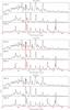 |
Fig. A.2 Top: same as Fig. A.1 for N II. Middle: same for O I. Bottom: same for Na I. |
| In the text | |
|
Fig. A.3 Top: same as Fig. A.1 for Mg I (red) and Mg II (green). Middle: same for Si I. Bottom: same for S I (red) and S II (green). |
| In the text | |
|
Fig. A.4 Top: same as Fig. A.1 for Ca II. Middle: same for Ti II. Bottom: same for Fe I (red), Fe II (green), and Fe III (blue). |
| In the text | |
|
Fig. A.5 Top: same as Fig. A.1 for Co II. Middle: same for Ni II. Bottom: same for all remaining elements (Ne, Al, Ar, Sc, V, Cr, Mn). |
| In the text | |
|
Fig. A.6 Top: same as Fig. A.1 for the Fe/Co/He zone (red is the total contribution, blue is the contribution by the core component). Middle: same for the Si/S zone. Bottom: same for the O/Si/S zone. |
| In the text | |
|
Fig. A.7 Top: same as Fig. A.1 for the O/Ne/Mg zone. Middle: same for the O/C zone. Bottom: same for the He/C zone. |
| In the text | |
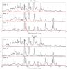 |
Fig. A.8 Top: same as Fig. A.1 for the He/N zone. Bottom: same for the H zone. |
| In the text | |
Current usage metrics show cumulative count of Article Views (full-text article views including HTML views, PDF and ePub downloads, according to the available data) and Abstracts Views on Vision4Press platform.
Data correspond to usage on the plateform after 2015. The current usage metrics is available 48-96 hours after online publication and is updated daily on week days.
Initial download of the metrics may take a while.