| Issue |
A&A
Volume 573, January 2015
|
|
|---|---|---|
| Article Number | A12 | |
| Number of page(s) | 44 | |
| Section | Astrophysical processes | |
| DOI | https://doi.org/10.1051/0004-6361/201423983 | |
| Published online | 10 December 2014 | |
Online material
Appendix A: Element and zone contributions
Figures A.1 to A.8 show the contribution by all major elements and zones to the emergent spectra of model 13G at 100, 300, and 500 days. These figures allow an overview of the various contributions and can be used for guidance in line identifications in other SNe.
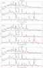 |
Fig. A.1
Top: contribution by H I lines (red) to the spectrum in model 13G (black), at 100, 300, and 500 days. Middle: same for He I. Bottom: same for C I. |
| Open with DEXTER | |
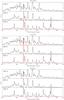 |
Fig. A.2
Top: same as Fig. A.1 for N II. Middle: same for O I. Bottom: same for Na I. |
| Open with DEXTER | |
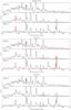 |
Fig. A.3
Top: same as Fig. A.1 for Mg I (red) and Mg II (green). Middle: same for Si I. Bottom: same for S I (red) and S II (green). |
| Open with DEXTER | |
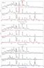 |
Fig. A.4
Top: same as Fig. A.1 for Ca II. Middle: same for Ti II. Bottom: same for Fe I (red), Fe II (green), and Fe III (blue). |
| Open with DEXTER | |
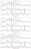 |
Fig. A.5
Top: same as Fig. A.1 for Co II. Middle: same for Ni II. Bottom: same for all remaining elements (Ne, Al, Ar, Sc, V, Cr, Mn). |
| Open with DEXTER | |
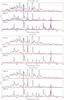 |
Fig. A.6
Top: same as Fig. A.1 for the Fe/Co/He zone (red is the total contribution, blue is the contribution by the core component). Middle: same for the Si/S zone. Bottom: same for the O/Si/S zone. |
| Open with DEXTER | |
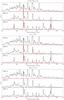 |
Fig. A.7
Top: same as Fig. A.1 for the O/Ne/Mg zone. Middle: same for the O/C zone. Bottom: same for the He/C zone. |
| Open with DEXTER | |
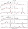 |
Fig. A.8
Top: same as Fig. A.1 for the He/N zone. Bottom: same for the H zone. |
| Open with DEXTER | |
Appendix B: Code updates
Appendix B.1: Atomic data
-
Mg I. Total radiative recombination rate updated, now from Badnell (2006). The dielectronic recombination rate is from Nussbaumer & Storey (1986). We compute specific recombination rates by applying the Milne relations to the TOPBASE photoionization cross sections (Cunto et al. 1993) for the first 30 (up to 3s6d(1D)) multiplets. For higher states, allocation of the remaining part of the total rate occurs in proportion to statistical weights, as described in Jerkstrand et al. (2011). There are some issues with applying the Milne relations to the TOPBASE bound-free cross sections; these include ionization to excited states, whereas we need the cross section for ionization to the ground state. The first excited state in Mg II has, however, an excitation energy of 4.42 eV, so for the moderate temperatures (T ≲ 104 K) of interest here, the contribution by the cross section at these high electron energies is small, and it should be a good approximation to use the full TOPBASE cross sections. Another complication is that the ionization thresholds given by TOPBASE are often somewhat offset from their correct values. One may choose to renormalize all energies to the correct threshold, here we have not done so (so we simply ignore any listed cross sections at energies below the ionization edge). We solve for statistical equilibrium for a 112 level atom (up to 15f(3F)). For higher levels our dataset on radiative transitions is incomplete and using a larger atomic model would therefore give a biased recombination cascade.
-
Na I. Total recombination rate from Verner & Ferland (1996). Specific recombination rates for first 16 terms (up to 6d(2D)) computed from TOPBASE photoionization cross sections (same as in Jerkstrand et al. (2011) but not fully clarified there). The collision strengths are from Trail et al. (1994) for the Na I D line, and from Park (1971) for the other transitions. The Trail et al. (1994) value is in good agreement with the recent calculation by Gao et al. (2010).
-
O I. Specific recombination rates from Nahar (1999) implemented for the first 26 terms (up to 5f(3F)).
-
S I. Forbidden line A-values updated with values from Froese Fischer et al. (2006) (via NIST).
-
Others. Added Ni III, with energy levels from Sugar & Corliss (1985) (up to 3d8(1G)) (via NIST), A-values from Garstang (1958) (via NIST), collision strengths (from ground multiplet only) from Bautista (2001). Added dielectronic recombination rates for Si I, Si II, S I, Ca I, Fe I, and Ni I (Shull & van Steenberg 1982). Added forbidden lines for Fe III, Co III, Al I, Al II, Ti I, Ti II, Ti III, Cr I, Cr II, Mn II, V I, V II, Sc I, Sc II (kurucz.harvard.edu). Added Fe III collision strengths from Zhang & Pradhan (1995b). Fe II collision strengths for the first 16 levels in Fe II now from Ramsbottom et al. (2007) (higher levels from Zhang & Pradhan 1995a and Bautista & Pradhan 1996).
Appendix C: Effective recombination rates
We calculate effective recombination rates (for use in the semi-analytical formulae derived in the text only, they have no use in the code itself) by computing the recombination cascade in the Case B and Case C limits, here taken to mean that transitions with A> 104 s-1 have infinite optical depth if the lower level belongs to the ground state multiplet (Case B), or to the ground multiplet or first excited multiplet (Case C), and all other transitions have zero optical depth. If all radiative de-excitation channels from a given level obtain infinite optical depth, we let the cascade go to the next level below (mimicking a collisional de-excitation).
Once the effective recombination rate to the parent state of a line has been computed, the rate to use for the line is this value times the fraction of de-excitations going to spontaneous radiative de-excitation in the line, which was computed with the same treatment as above. For all lines analyzed in this paper this fraction is very close to unity.
Appendix C.1: Oxygen
We solve for a 135 level atom (up to 8d(3D)), using total and specific recombination rates from Nahar (1999), which include both radiative and dielectronic recombination. The specific recombination rates were implemented for principal quantum numbers n = 1−5 (first 26 terms), with rates for higher levels being allocated in proportion to the statistical weights.
The resulting values for the effective recombination rates are compared with those computed by Maurer & Mazzali (2010) in Table C.1. The Maurer & Mazzali (2010) values include only radiative recombination, bit since dielectronic contribution is relatively weak below 104 K, this is a reasonable approximation. Table C.1 shows that the agreement is good, within a factor of two for all lines at all temperatures.
Computed effective recombination rates (units in cm3 s-1) for the O I λ7774, O I λ9263, O I λ1.129 μm, O I λ1.130 μm, and O I λ1.316 μm lines.
Appendix C.2: Magnesium
Table C.2 shows the effective recombination rates computed for Mg I. Note the turn-up at higher temperatures, caused by the dielectronic contribution.
Computed effective recombination rates (units cm3 s-1) for the Mg I] λ4571 and Mg I λ1.504 μm lines.
Appendix D: Ejecta models
The mass and composition of the ejecta models used are presented in Tables D.1–D.4.
Zone masses (in M⊙) in the models.
Zone compositions (mass fractions) of the 12 M⊙ models.
© ESO, 2014
Current usage metrics show cumulative count of Article Views (full-text article views including HTML views, PDF and ePub downloads, according to the available data) and Abstracts Views on Vision4Press platform.
Data correspond to usage on the plateform after 2015. The current usage metrics is available 48-96 hours after online publication and is updated daily on week days.
Initial download of the metrics may take a while.