| Issue |
A&A
Volume 573, January 2015
|
|
|---|---|---|
| Article Number | A50 | |
| Number of page(s) | 12 | |
| Section | Extragalactic astronomy | |
| DOI | https://doi.org/10.1051/0004-6361/201322906 | |
| Published online | 17 December 2014 | |
Multiwavelength observations of Mrk 501 in 2008⋆
1 IFAE, Edifici Cn., Campus UAB, 08193 Bellaterra, Spain
2 Università di Udine, and INFN Trieste, 33100 Udine, Italy
3 INAF National Institute for Astrophysics, 00136 Rome, Italy
4 Università di Siena, and INFN Pisa, 53100 Siena, Italy
5 Croatian MAGIC Consortium, Rudjer Boskovic Institute, University of Rijeka and University of Split, 10000 Zagreb, Croatia
6 Max-Planck-Institut für Physik, 80805 München, Germany
7 Universidad Complutense, 28040 Madrid, Spain
8 Inst. de Astrofísica de Canarias, 38200 La Laguna, Tenerife, Spain
9 University of Lodz, 90236 Lodz, Poland
10 Deutsches Elektronen-Synchrotron (DESY), 15738 Zeuthen, Germany
11 ETH Zurich, 8093 Zurich, Switzerland
12 Universität Würzburg, 97074 Würzburg, Germany
13 Centro de Investigaciones Energéticas, Medioambientales y Tecnológicas, 28040 Madrid, Spain
14 Technische Universität Dortmund, 44221 Dortmund, Germany
15 Inst. de Astrofísica de Andalucía (CSIC), 18080 Granada, Spain
16 Università di Padova and INFN, 35131 Padova, Italy
17 Università dell’Insubria, Como, 22100 Como, Italy
18 Unitat de Física de les Radiacions, Departament de Física, and CERES-IEEC, Universitat Autònoma de Barcelona, 08193 Bellaterra, Spain
19 Institut de Ciències de l’Espai (IEEC-CSIC), 08193 Bellaterra, Spain
20 Finnish MAGIC Consortium, Tuorla Observatory, University of Turku and Department of Physics, University of Oulu, 900147 Oulu, Finland
21 Japanese MAGIC Consortium, Division of Physics and Astronomy, Kyoto University, 606-8501 Kyoto, Japan
22 Inst. for Nucl. Research and Nucl. Energy, 1784 Sofia, Bulgaria
23 Universitat de Barcelona (ICC/IEEC), 08028 Barcelona, Spain
24 Università di Pisa, and INFN Pisa, 56126 Pisa, Italy
25 Now at École polytechnique fédérale de Lausanne (EPFL), Lausanne, Switzerland
26 Now at Department of Physics & Astronomy, UC Riverside, CA 92521, USA
27 Now atFinnish Centre for Astronomy with ESO (FINCA), Turku, Finland
28 Also at INAF-Trieste
29 Also at Instituto de Fisica Teorica, UAM/CSIC, 28049 Madrid, Spain
30 Now at Stockholms universitet, Oskar Klein Centre for Cosmoparticle Physics, Sweden
31 Now at GRAPPA Institute, University of Amsterdam, 1098 XH Amsterdam, The Netherlands
32 Department of Physics, Washington University, St. Louis, MO 63130, USA
33 Fred Lawrence Whipple Observatory, Harvard-Smithsonian Center for Astrophysics, Amado, AZ 85645, USA
34 Department of Physics and Astronomy and the Bartol Research Institute, University of Delaware, Newark, DE 19716, USA
35 School of Physics, University College Dublin, Belfield, Dublin 4, Ireland
36 Santa Cruz Institute for Particle Physics and Department of Physics, University of California, Santa Cruz, CA 95064, USA
37 Institute of Physics and Astronomy, University of Potsdam, 14476 Potsdam-Golm, Germany
38 Astronomy Department, Adler Planetarium and Astronomy Museum, Chicago, IL 60605, USA
39 Department of Physics, Purdue University, West Lafayette, IN 47907, USA
40 Department of Physics, Grinnell College, Grinnell, IA 50112-1690, USA
41 School of Physics and Astronomy, University of Minnesota, Minneapolis, MN 55455, USA
42 Department of Astronomy and Astrophysics, 525 Davey Lab, Pennsylvania State University, University Park, PA 16802, USA
43 School of Physics, National University of Ireland Galway, University Road, Galway, Ireland
44 Physics Department, McGill University, Montreal, QC H3A 2T8, Canada
45 Department of Physics and Astronomy, University of Iowa, Van Allen Hall, Iowa City, IA 52242, USA
46 Department of Physics and Astronomy, DePauw University, Greencastle, IN 46135-0037, USA
47 Department of Physics and Astronomy, University of Utah, Salt Lake City, UT 84112, USA
48 Department of Physics and Astronomy, Iowa State University, Ames, IA 50011, USA
49 Department of Physics and Astronomy, University of California, Los Angeles, CA 90095, USA
50 Saha Institute of Nuclear Physics, 700064 Kolkata, India
51 School of Physics and Center for Relativistic Astrophysics, Georgia Institute of Technology, 837 State Street NW, Atlanta, GA 30332-0430, USA
52 Department of Life and Physical Sciences, Galway-Mayo Institute of Technology, Dublin Road, Galway, Ireland
53 Department of Physics and Astronomy, Barnard College, Columbia University, NY 10027, USA
54 Physics Department, Columbia University, New York, NY 10027, USA
55 Instituto de Astronomia y Fisica del Espacio, Casilla de Correo 67 – Sucursal 28, (C1428ZAA) Ciudad Autnoma de Buenos Aires, Argentina
56 Physics Department, California Polytechnic State University, San Luis Obispo, CA 94307, USA
57 Department of Applied Physics and Instrumentation, Cork Institute of Technology, Bishopstown, Cork, Ireland
58 Enrico Fermi Institute, University of Chicago, Chicago, IL 60637, USA
59 Argonne National Laboratory, 9700 S. Cass Avenue, Argonne, IL 60439, USA
60 INAF, Osservatorio Astronomico di Torino, 10025 Pino Torinese (TO), Italy
61 Space Sciences Laboratory, 7 Gauss Way, University of California, Berkeley, CA 94720-7450, USA
62 ASI-Science Data Center, via del Politecnico, 00133 Rome, Italy
63 Department of Astronomy, University of Michigan, Ann Arbor, MI 48109-1042, USA
64 Astron. Inst., St.-Petersburg State Univ., 198504 St. Petersburg, Russia
65 Pulkovo Observatory, 196140 St. Petersburg, Russia
66 Isaac Newton Institute of Chile, St.-Petersburg Branch, Russia
67 Graduate Institute of Astronomy, National Central University, 300 Jhongda Rd., 32001 Jhongli, Taiwan
68 Moscow M.V. Lomonosov State University, Sternberg Astronomical Institute, Russia
69 Abastumani Observatory, Mt. Kanobili, 0301 Abastumani, Georgia
70 Landessternwarte, Zentrum für Astronomie der Universität Heidelberg, Königstuhl 12, 69117 Heidelberg, Germany
71 School of Cosmic Physics, Dublin Institute For Advanced Studies, Ireland
72 INAF–Osservatorio Astrofisico di Catania, Italy
73 Aalto University Metsähovi Radio Observatory Metsähovintie 114, 02540 Kylmälä, Finland
74 Finnish Centre for Astronomy with ESO (FINCA) University of Turku Väisäläntie 20, 21500 Piikkiö, Finland
75 INAF Istituto di Radioastronomia, 40129 Bologna, Italy
76 University of Trento, Department of Physics, 38050 Povo, Trento, Italy
77 Max-Planck-Institut für Radioastronomie, Auf dem Hügel 69, 53121 Bonn, Germany
78 Astro Space Center of the Lebedev Physical Institute, 117997 Moscow, Russia
79 Engelhardt Astronomical Observatory, Kazan Federal University Tatarstan Russia
80 Aalto University Department of Radio Science and Engineering, PO Box 13000, 00076 Aalto, Finland
Received: 24 October 2013
Accepted: 15 July 2014
Abstract
Context. Blazars are variable sources on various timescales over a broad energy range spanning from radio to very high energy (>100 GeV, hereafter VHE). Mrk 501 is one of the brightest blazars at TeV energies and has been extensively studied since its first VHE detection in 1996. However, most of the γ-ray studies performed on Mrk 501 during the past years relate to flaring activity, when the source detection and characterization with the available γ-ray instrumentation was easier toperform.
Aims. Our goal is to characterize the source γ-ray emission in detail, together with the radio-to-X-ray emission, during the non-flaring (low) activity, which is less often studied than the occasional flaring (high) activity.
Methods. We organized a multiwavelength (MW) campaign on Mrk 501 between March and May 2008. This multi-instrument effort included the most sensitive VHE γ-ray instruments in the northern hemisphere, namely the imaging atmospheric Cherenkov telescopes MAGIC and VERITAS, as well as Swift, RXTE, the F-GAMMA, GASP-WEBT, and other collaborations and instruments. This provided extensive energy and temporal coverage of Mrk 501 throughout the entire campaign.
Results. Mrk 501 was found to be in a low state of activity during the campaign, with a VHE flux in the range of 10%–20% of the Crab nebula flux. Nevertheless, significant flux variations were detected with various instruments, with a trend of increasing variability with energy and a tentative correlation between the X-ray and VHE fluxes. The broadband spectral energy distribution during the two different emission states of the campaign can be adequately described within the homogeneous one-zone synchrotron self-Compton model, with the (slightly) higher state described by an increase in the electron number density.
Conclusions. The one-zone SSC model can adequately describe the broadband spectral energy distribution of the source during the two months covered by the MW campaign. This agrees with previous studies of the broadband emission of this source during flaring and non-flaring states. We report for the first time a tentative X-ray-to-VHE correlation during such a low VHE activity. Although marginally significant, this positive correlation between X-ray and VHE, which has been reported many times during flaring activity, suggests that the mechanisms that dominate the X-ray/VHE emission during non-flaring-activity are not substantially different from those that are responsible for the emission during flaring activity.
Key words: astroparticle physics / BL Lacertae objects: individual: Mrk 501 / gamma rays: general
The data for Figs. 2 and 5 are only available at the CDS via anonymous ftp to cdsarc.u-strasbg.fr (130.79.128.5) or via http://cdsarc.u-strasbg.fr/viz-bin/qcat?J/A+A/573/A50
Corresponding authors: D. Paneque, e-mail: This email address is being protected from spambots. You need JavaScript enabled to view it. ; K. Satalecka, e-mail: This email address is being protected from spambots. You need JavaScript enabled to view it. ; and N. Mankuzhiyil, e-mail: This email address is being protected from spambots. You need JavaScript enabled to view it. † Deceased.
Deceased.
© ESO, 2014
1. Introduction
Almost one third of the sources detected at very high energy (>100 GeV, hereafter VHE) are BL Lac objects, that is, active galactic nuclei (AGN) that contain relativistic jets pointing approximately in the direction of the observer. Their spectral energy distribution (SED) shows a continuous emission with two broad peaks: one in the UV-to-soft X-ray band, and a second one in the GeV–TeV range. They display no or only very weak emission lines at optical/UV energies. One of the most interesting aspects of BL Lacs is their flux variability, observed in all frequencies and on different timescales ranging from weeks down to minutes, which is often accompanied by spectral variability.
Mrk 501 is a well-studied nearby (redshift z = 0.034) BL Lac that was first detected at TeV energies by the Whipple collaboration in 1996 (Quinn et al. 1996). In the following years it has been observed and detected in VHE γ-rays by many other Cherenkov telescope experiments. During 1997 it showed an exceptionally strong outburst with peak flux levels up to ten times the Crab nebula flux, and flux-doubling timescales down to 0.5 day (Aharonian et al. 1999). Mrk 501 also showed strong flaring activity at X-ray energies during that year. The X-ray spectrum was very hard (α< 1, with Fν ∝ ν− α), with the synchrotron peak found to be at ~100 keV, about 2 orders of magnitude higher than in previous observations (Pian et al. 1998). In the following years, Mrk 501 showed only low γ-ray emission (of about 20–30% of the Crab nebula flux), apart from a few single flares of higher intensity. In 2005, the MAGIC telescope observed Mrk 501 during another high-emission state which, although at a lower flux level than that of 1997, showed flux variations of an order of magnitude and previously not recorded flux-doubling timescales of only few minutes (Albert et al. 2007a).
Mrk 501 has been monitored extensively in X-ray (e.g., Beppo SAX 1996–2001, Massaro et al. 2004) and VHE (e.g., Whipple 1995–1998, Quinn et al. 1999, and HEGRA 1998–1999, Aharonian et al. 2001), and many studies have been conducted a posteriori using these observations (e.g., Gliozzi et al. 2006). With the last-generation Cherenkov telescopes (before the new generation of Cherenkov telescopes started to operate in 2004), coordinated multiwavelength (MW)observations were mostly focused on high VHE activity states (e.g., Krawczynski et al. 2000; Tavecchio et al. 2001), with few campaigns also covering low VHE states (e.g., Kataoka et al. 1999; Sambruna et al. 2000). The data presented here were taken between March 25 and May 16, 2008 during a MW campaign covering radio (Effelsberg, IRAM, Medicina, Metsähovi, Noto, RATAN-600, UMRAO, VLBA), optical (through various observatories within the GASP-WEBT program), UV (Swift/UVOT), X-ray (RXTE/PCA, Swift/XRT and Swift/BAT), and γ-ray (MAGIC, VERITAS) energies. This MW campaign was the first to combine such a broad energy and time coverage with higher VHE sensitivity and was conducted when Mrk 501 was not in a flaring state.
The paper is organized as follows: in Sect. 2 we describe the participating instruments and the data analyses. Sections 3–5 are devoted to the multifrequency variability and correlations. In Sect. 6 we report on the modeling of the SED data within a standard scenario for this source, and in Sect. 7 we discuss the implications of the experimental and modeling results.
2. Details of the campaign: participating instruments and temporal coverage
The list of instruments that participated in the campaign is reported in Table 1. Figure 1 shows the time coverage as a function of the energy range for the instruments and observations used to produce the light curves presented in Fig. 2 and the SEDs shown in Fig. 5.
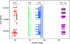 |
Fig. 1 Time and energy coverage during the multifrequency campaign. For the sake of clarity, the shortest observing time displayed in the plot was set to half a day, and different colors were used to display different energy ranges. The correspondence between energy ranges and instruments is provided in Table 1. |
2.1. Radio instruments
In this campaign, the radio frequencies were covered by various single-dish telescopes: the Effelsberg 100 m radio telescope, the 32 m Medicina radio telescope, the 14 m Metsähovi radio telescope, the 32 m Noto radio telescope, the 26 m University of Michigan Radio Astronomy Observatory (UMRAO), and the 600 m ring radio telescope RATAN-600. Details of the observing strategy and data reduction are given by Fuhrmann et al. (2008); Angelakis et al. (2008, Effelsberg), Teräsranta et al. (1998, Metsähovi), Aller et al. (1985, UMRAO), Venturi et al. (2001, Medicina and Noto), and Kovalev et al. (1999, RATAN-600.
2.2. Optical instruments
The coverage at optical frequencies was provided by various telescopes around the world within the GASP-WEBT program (e.g., Villata et al. 2008, 2009). In particular, the following observatories contributed to this campaign: Abastumani, Lulin, Roque de los Muchachos (KVA), St. Petersburg, Talmassons, and the Crimean observatory. See Table 1 for more details. All the observations were performed at the R band, using the calibration stars reported by Villata et al. (1998). The Galactic extinction was corrected for with the coefficients given by Schlegel et al. (1998). The flux was also corrected for the estimated contribution from the host galaxy, 12 mJy for an aperture radius of 7.5 arcsec (Nilsson et al. 2007).
2.3. Swift/UVOT
The Swift UltraViolet and Optical Telescope (UVOT; Roming et al. 2005) analysis was performed including all the available observations between MJD 54 553 and 54 599. The instrument cycled through each of the three optical pass bands V,B, and U, and the three ultraviolet pass bands UVW1, UVM2, and UVW2. The observations were performed with exposure times ranging from 50 to 900 s with a typical exposure of 150 s. Data were taken in the image mode, where the image is directly accumulated onboard, discarding the photon timing information, and hence reducing the telemetry volume.
The photometry was computed using an aperture of 5 arcsec following the general prescription of Poole et al. (2008), introducing an annulus background region (inner and outer radii 20 and 30 arcsec), and it was corrected for Galactic extinction E(B − V) = 0.019 mag (Schlegel et al. 1998) in each spectral band (Fitzpatrick 1999).
Note that for each filter the integrated flux was computed by using the related effective frequency, and not by folding the filter transmission with the source spectrum. This might produce a moderate overestimate of the integrated flux of about 10%. The total systematic uncertainty is estimated to be ≲18%.
2.4. Swift/XRT
The Swift X-ray Telescope (XRT; Burrows et al. 2005) pointed to Mrk 501 18 times in the time interval spaning from MJD 54 553 to 54 599. Each observation was about 1–2 ks long, with a total exposure time of 26 ks. The observations were performed in windowed timing (WT) mode to avoid pile-up, which could be a problem for the typical count rates from Mrk 501, which are about ~5 cps (Stroh & Falcone 2013).
The XRT data set was first processed with the XRTDAS software package (v.2.8.0) developed at the ASI Science Data Center (ASDC) and distributed by HEASARC within the HEASoft package (v. 6.13). Event files were calibrated and cleaned with standard filtering criteria with the xrtpipeline task.
The average spectrum was extracted from the summed cleaned event file. Events for the spectral analysis were selected within a circle of 20 pixel (~46 arcsec) radius, which encloses about 80% of the PSF, centered on the source position.
The ancillary response files (ARFs) were generated with the xrtmkarf task, applying corrections for the PSF losses and CCD defects using the cumulative exposure map. The latest response matrices (v. 014) available in the Swift CALDB1 were used. Before the spectral fitting, the 0.3–10 keV source energy spectra were binned to ensure a minimum of 20 counts per bin. The spectra were corrected for absorption with a neutral hydrogen column density NH fixed to the Galactic 21 cm value in the direction of the source, namely 1.56 × 1020 cm-2 (Kalberla et al. 2005). When calculating the SED data points, the original spectral data were binned by combining 40 adjacent bins with the XSPEC command setplot rebin. The error associated to each binned SED data point was calculated adding in quadrature the errors of the original bins. The X-ray fluxes in the 0.3–10 keV band were retrieved from the log-parabola function fitted to the spectrum using the XSPEC command flux.
2.5. RXTE/PCA
The Rossi X-ray Timing Explorer (RXTE; Bradt et al. 1993) satellite performed 29 pointings on Mrk 501 during the time interval from MJD 54 554 to 54 601. Each pointing lasted 1.5 ks. The data analysis was performed using the FTOOLS v6.9 and following the procedures and filtering criteria recommended by the RXTE Guest Observer Facility2 after September 2007. The average net count rate from Mrk 501 was about 5 cps per proportional counter unit (PCU) in the energy range 3–20 keV, with flux variations typically lower than a factor of two. Consequently, the observations were filtered following the conservative procedures for faint sources. For details on the analysis of faint sources with RXTE, see the online Cook Book3. In the data analysis, only the first xenon layer of PCU2 was used to increase the quality of the signal. We used the package pcabackest to model the background, the package saextrct to produce spectra for the source and background files and the script pcarsp to produce the response matrix. As with the Swift/XRT analysis, here we also used a hydrogen-equivalent column density NH of 1.56 × 1020 cm-2 (Kalberla et al. 2005). However, since the PCA bandpass starts at 3 keV, the value used for NH does not significantly affect our results. The RXTE/PCA X-ray fluxes were retrieved from the power-law function fitted to the spectrum using the XSPEC command flux.
2.6. Swift/BAT
The Swift Burst Alert Telescope (BAT; Barthelmy et al. 2005) analysis results presented in this paper were derived with all the available data during the time interval from MJD 54 548 to 54 604. The seven-day binned fluxes shown in the light curves were determined from the weighted average of the daily fluxes reported in the NASA Swift/BAT web page4. On the other hand, the spectra for the three time intervals defined in Sect. 3 were produced following the recipes presented by Ajello et al. (2008, 2009b). The uncertainty in the Swift/BAT flux/spectra is large because Mrk 501 is a relatively faint X-ray source and is therefore difficult to detect above 15 keV on weekly timescales.
2.7. MAGIC
MAGIC is a system of two 17 m diameter imaging atmospheric Cherenkov telescopes (IACTs), located at the Observatory Roque de los Muchachos, in the Canary island of La Palma (28.8 N, 17.8 W, 2200 m a.s.l.). The system has been operating in stereo mode since 2009 (Aleksić et al. 2011). The observations reported in this manuscript were performed in 2008, hence when MAGIC consisted on a single telescope. The MAGIC-I camera contained 577 pixels and had a field of view of 3.5°. The inner part of the camera (radius ~1.1°) was equipped with 397 PMTs with a diameter of 0.1° each. The outer part of the camera was equipped with 180 PMTs of 0.2° diameter. MAGIC-I working as a stand-alone instrument was sensitive over an energy range of 50 GeV to 10 TeV with an energy resolution of 20%, an angular PSF of about 0.1° (depending on the event energy) and a sensitivity of 2% the integral flux of the Crab nebula in 50 h of observation (Albert et al. 2008b).
MAGIC observed Mrk 501 during 20 nights between 2008 March 29 and 2008 May 13 (from MJD 54 554 to 54 599). The observations were performed in ON mode, which means that the source is located exactly at the center in the telescope PMT camera. The data were analyzed using the standard MAGIC analysis and reconstruction software MARS (Albert et al. 2008a; Aliu et al. 2009; Zanin et al. 2013). The data surviving the quality cuts amount to a total of 30.4 h. The derived spectrum was unfolded to correct for the effects of the limited energy resolution of the detector and possible bias (Albert et al. 2007b) using the most recent (March 2014) release of the MAGIC unfolding routines, which take into account the distribution of the observations in zenith and azimuth for a correct effective collection area recalculation. The resulting spectrum is characterized by a power-law function with spectral index (−2.42 ± 0.05) and normalization factor (at 1 TeV) of (7.4 ± 0.2) × 10-12 cm-2 s-1 TeV-1 (see Appendix A). The photon fluxes for the individual observations were computed for a photon index of 2.5, yielding an average flux of about 20% of that of the Crab nebula above 300 GeV, with relatively mild (typically lower than factor 2) flux variations.
2.8. VERITAS
VERITAS is an array of four IACTs, each 12 m in diameter, located at the Fred Lawrence Whipple Observatory in southern Arizona, USA (31.7 N, 110.9 W). Full four-telescope operations began in 2007. All observations presented here were taken with all four telescopes operational, and prior to the relocation of the first telescope within the array layout (Perkins et al. 2009). Each VERITAS camera contains 499 pixels (each with an angular diameter of 0.15°) and has a field of view of 3.5°. VERITAS is sensitive over an energy range of 100 GeV to 30 TeV with an energy resolution of 15%–20% and an angular resolution (68% containment) lower than 0.1° per event.
The VERITAS observations of Mrk 501 presented here were taken on 16 nights between 2008 April 1 and 2008 May 13. After applying quality-selection criteria, the total exposure is 6.2 h live time. Data-quality selection requires clear atmospheric conditions, based on infrared sky temperature measurements, and normal hardware operation. All data were taken during moon-less periods in wobble mode with pointings of 0.5° from the blazar alternating from north, south, east, and west to enable simultaneous background estimation and reduce systematics (Aharonian et al. 2001). Data reduction followed the methods described by Acciari et al. (2008). The spectrum obtained with the full dataset is described by a power-law function with spectral index (−2.47 ± 0.10) and normalization factor (at 1 TeV) of (9.4 ± 0.6) × 10-12 cm-2 s-1 TeV-1 (see Appendix A). In the calculation of the photon fluxes integrated above 300 GeV for the single VERITAS observations, we used a photon index of 2.5.
3. Light curves
Figure 2 shows the light curves for all of the instruments that participated in the campaign. The five panels from top to bottom present the light curves grouped into five energy ranges: radio, optical, X-ray, hard X-ray, and VHE.
The multifrequency light curves show little variability; during this campaign there were no outbursts of the magnitude observed in the past for this object (e.g., Krawczynski et al. 2000; Albert et al. 2007a). Around MJD 54 560, there is an increase in the X-rays activity, with a Swift/XRT flux (in the energy range 0.3–10 keV) of ~1.3 × 10⁻¹⁰ erg cm-2 s-1 before, and ~1.7 × 10⁻¹⁰ erg cm-2 s-1 after this day. The measured X-ray flux during this campaign is well below ~2.0 × 10⁻¹⁰ erg cm-2 s-1, which is the average X-ray flux measured with Swift/XRT during the time interval of 2004 December 22 through 2012 August 31, which was reported in Stroh & Falcone (2013). In the VHE domain, the γ-ray flux above 300 GeV is mostly below ~2 × 10-11 ph cm-2 s-1 before MJD 54 560, and above ~2 × 10-11 ph cm-2 s-1 after this day. The variability in the multifrequency activity of the source is discussed in Sect. 4, while the correlation among energy bands is reported in Sect. 5.
For the spectral analysis presented in Sect. 6, we divided the data set into three time intervals according to the X-ray flux level (i.e., low/high flux before/after MJD 54 560) and the data gap at most frequencies in the time interval MJD 54 574–54 579 (which is due to the difficulty of observing with IACTs during the nights with moonlight).
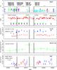 |
Fig. 2 Multifrequency light curve for Mrk 501 during the entire campaign period. The panels from top to bottom show the radio, optical and UV, X-ray, hard X-ray, and VHE γ-ray bands. The thick black vertical lines in all the panels delimit the time intervals corresponding to the three different epochs (P1, P2, and P3) used for the SED model fits in Sect. 6. The horizontal dashed line in the bottom panel depicts 10% of the flux of the Crab nebula above 300 GeV (Albert et al. 2008b). |
4. Variability
We followed the description given by Vaughan et al. (2003) to quantify the flux variability by means of the fractional variability parameter Fvar. To account for the individual flux measurement errors (σerr,i), the “excess variance” (Edelson et al. 2002) was used as an estimator of the intrinsic source flux variance. This is the variance after subtracting the contribution expected from measurement statistical uncertainties. This analysis does not account for systematic uncertainties. Fvar was derived for each participating instrument individually, which covered an energy range from radio frequencies at ~8 GHz up to very high energies at ~10 TeV. Fvar is calculated as (1)where ⟨ Fγ ⟩ denotes the average photon flux, S the standard deviation of the N flux measurements and
  the mean squared error, all determined for a given instrument (energy bin). The uncertainty of Fvar is estimated according to
 (2)where \begin{lxirformule}$err(\sigma^{2}_{\mathrm{NXS}})$\end{lxirformule} is given by Eq. (11) in Vaughan et al. (2003),
 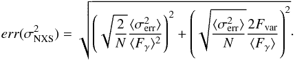 (3)As reported in Sect. 2.2 in Poutanen et al. (2008), this prescription of computing ΔFvar is more appropriate than that given by Eq. (B2) in Vaughan et al. (2003), which is not correct when the error in the excess variance is similar to or larger than the excess variance. For this data set, we found that the prescription from Poutanen et al. (2008), which is used here, leads to ΔFvar that are ~40% smaller than those computed with Eq. (B2) in Vaughan et al. (2003) for the energy bands with the lowest
  , while for most of the data points (energy bands) the errors are only ~20% smaller, and for the data points with the highest they are only few % smaller.
Figure 3 shows the Fvar values derived for all instruments that participated in the MW campaign. The flux values that were used are displayed in Fig. 2. All flux values correspond to measurements performed on minutes or hour timescales, except for Swift/BAT, whose X-ray fluxes correspond to a seven-day integration because of the somewhat moderate sensitivity of this instrument to detect Mrk 501. Consequently, Swift/BAT data cannot probe the variability on timescales as short as the other instruments, and hence Fvar might be underestimated for this instrument. We obtained negative excess variance ( larger than S2) for the lowest frequencies of several radio telescopes. A negative excess variance can occur when there is little variability (in comparison with the uncertainty of the flux measurements) and/or when the errors are slightly overestimated. A negative excess variance can be interpreted as no signature for variability in the data of that particular instrument, either because a) there was no variability; or b) the instrument was not sensitive enough to detect it. Figure 3 only shows the fractional variance for instruments with positive excess variance.
At radio frequencies, there is essentially no variability: all bands and instruments show Fvar close to zero, with the exception of the of RATAN (22 GHz) and Metsähovi (37 GHz), which show Fvar ~ 7 ± 2%. A possible reason for this apparently significant variability is unaccounted-for errors due to variable weather conditions, which can easily add a random extra fluctuation (day-by-day) of a few percent. However, it is worth mentioning that this flickering behavior has been observed several times with Metsähovi at 37 GHz, for example, in Mrk 501 and also in Mrk 421, while it is rare in other types of blazar objects; hence there is a chance that the measured fractional variability is dominated by a real flickering in the high-frequency radio emission of Mrk 501. More studies on this aspect will be reported elsewhere.
During the 2008 campaign on Mrk 501, we measured variability in the optical, X-ray, and gamma-ray energy bands. The plot also shows some evidence that the observed flux variability increases with energy: in the optical R band (ground-based telescopes) and the three UV filters from Swift/UVOT the variability is ~3%, at X-rays it is ~13%, and at VHE it is ~20%, although affected by relatively large error bars (because of the statistical uncertainties in the individual flux measurements).
5. Multifrequency cross-correlations
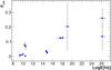 |
Fig. 3 Fractional variability parameter Fvar vs. energy covered by the various instruments. Fvar was derived using the individual single-night flux measurements except for Swift/BAT, for which, because of the limited sensitivity, we used data integrated over one week. Vertical bars denote 1σ uncertainties, horizontal bars indicate the approximate energy range covered by the instruments. |
We used the discrete correlation function (DCF) proposed by Edelson & Krolik (1988) to study the multifrequency cross-correlations between the different energy bands. The DCF quantifies the temporal correlation as a function of the time lag between two light curves, which can give us a deeper insight into the acceleration processes in the source. For example, these time lags may occur as a result of spatially separated emission regions of the individual flux components (as expected, for example, in external inverse Compton models), or may be caused by the energy-dependent cooling time-scales of the emitting electrons.
There are two important properties of the DCF method. First, it can be applied to unevenly sampled data (as in this campaign), meaning that the correlation function is defined only for lags for which the measured data exist, which makes an interpolation of the data unnecessary. The result is a correlation function that is a set of discrete points binned in time. Second, the errors in the individual flux measurements (which contribute to the dispersion in the flux values) are naturally taken into account. The latter characteristic is a big advantage over the commonly used Pearson correlation function. The main caveat of the DFC method is that the correlation function is not continuous and that care needs to be taken when defining the time bins to achieve a reasonable balance between the required time resolution and accuracy of DCF. Given the many two-day (sometimes three-day) time gaps in the X-ray and VHE observations from this MW campaign (see Figs. 1 and 2), we selected a time bin of three days to compute the DCF with minimal impact of these observational gaps. Moreover, given the relatively low variability reported in Fig. 2, an estimation of DCF would not benefit from a smaller time bin.
Using the data collected in this campaign, we derived the DCF for all different combinations of instruments and energy regions and also for artificially introduced time lags (ranging from –21 to +21 days) between the individual light curves. Significant correlations were found only for the pairs RXTE/PCA – Swift/XRT and also (less significant) RXTE/PCA with MAGIC and VERITAS (Figs. 4a and b). In both cases, the highest DCF values are obtained for a zero time lag, with a value of 0.71 ± 0.22 (RXTE/PCA – Swift/XRT) and 0.45 ± 0.15 (RXTE/PCA – MAGIC and VERITAS), which implies positive correlations with a significance of 3.2 and 3.0 standard deviations.
As discussed in Uttley et al. (2003), the errors in the DCF computed as prescribed in Edelson & Krolik (1988) might not be appropriate for determining the significance of the DCF when the individual light-curve data points are correlated red-noise data. Depending on the power spectral density (PSD) and the sampling pattern, the significance as calculated by Edelson & Krolik (1988) might therefore overestimate the real significance. To derive an independent estimate of the real significance of the correlation peaks we used the dedicated Monte Carlo approach described below.
 |
Fig. 4 Discrete correlation function for time lags from –21 to +21 days in steps of 3 days. The (black) data points and errors are the DCF values computed according to the prescription given by Edelson & Krolik (1988). The (blue) dashed and the (red) dotted curves depict the 95% and 99% confidence intervals for random correlations resulting from the dedicated Monte Carlo analysis described in Sect. 5. |
First we generated a large set of simulated light curves using the method of Timmer & Koenig (1995) following the prescription of Uttley et al. (2002). As a model for the PSD we assumed a simple power-law shape5, and generated for each observed light curve and for each PSD model (we varied the PSD slope in the range –1.0 to –2.5 in steps of 0.1) 1000 simulated light curves. The simulated light curves were then resampled using the sampling pattern of the observed light curve. By applying the psresp method (Uttley et al. 2002) we tried to determine the best-fitting model for the PSD. This involves the following steps in addition to the light-curve simulation and resampling: the PSD of the observed light curve, as well as the PSD of each simulated light curve, is calculated as the square of the modulus of the discrete Fourier transform of the (mean subtracted) light curve, as prescribed in Uttley et al. (2002). A χ2 analysis is then used to determine the model that best fits the data. Given the short frequency range, the uneven sampling and the presence of large gaps (particularly in the VHE data), it was not possible to constrain the PSD shape very tightly. The best-fitting models are power laws with indices 1.4 (VHE) and 1.5 (X-rays), however, any power law with an index between 1.0 and 1.9 fits the data reasonably well. The RXTE/PCA light curve is sampled more often and regularly than the other VHE and X-ray light curves, and moreover, Kataoka et al. (2001) found an X-ray PSD slope similar to ours (1.37 ± 0.16) in the frequency range probed here. Therefore we used the simulated RXTE/PCA light curves with a PSD slope of –1.5 to ascertain the confidence levels in the DCF calculation. We cross-correlated each of the 1000 simulated RXTE/PCA light curves with the observed VHE (MAGIC&VERITAS) and Swift/XRT light curves. The 95 and 99% limits of the distribution of simulated RXTE/PCA light curves when correlated with the real VHE and Swift/XRT light curves are plotted in Figs. 4a and b as blue dashed and red dotted lines, respectively. The correlation peaks at time lag = 0 are higher than >99% of the simulated data for the DCF for RXTE/PCA correlated with Swift/XRT, and ~99% for the simulated data for the DCF for RXTE/PCA with VHE (MAGIC&VERITAS). Given that a 99% confidence level is equivalent to 2.5 standard deviations, this result agrees reasonably well with the significances of ~3 standard deviations estimated from the Edelson & Krolik DCF errors, thus indicating that in this case the red-noise nature and the sampling of the light curve do not have a very strong influence. There are no other peaks or dips in the DCF between VHE and X-rays that appear significant.
The positive correlation in the fluxes from Swift/XRT and RXTE/PCA is expected because of the proximity (and overlap) of the energy coverage of these two instruments (see Table 1), while the correlated behavior between RXTE/PCA and MAGIC/VERITAS suggests that the X-ray and VHE emission are co-spatial and produced by the same population of high-energy particles. The correlation between the X-ray and VHE band has been reported many times in the past (e.g., Krawczynski et al. 2000; Tavecchio et al. 2001; Gliozzi et al. 2006; Albert et al. 2007a), but only when Mrk 501 showed flaring VHE activity with VHE fluxes higher than the flux of the Crab nebula. An X-ray/VHE correlation when the source shows a VHE flux below 0.5 Crab has never been shown until now.
6. SED modeling
Using the multifrequency data, we derived time-resolved SEDs for three different periods that were defined according to the observed X-ray flux during this campaign (see Sect. 3). The Swift, RXTE, MAGIC, and VERITAS spectral results for the three periods are reported in Appendix A. The X-ray spectral results reported in Tables A.1 and A.2 show that Mrk 501 became brighter and harder in P2/P3 than in P1. The VHE spectra reported in Tables A.3 and A.4 show that the MAGIC and VERITAS spectral results agree with each other within statistical uncertainties (despite the slightly different temporal coverage). The VHE spectral results do not show any significant spectral hardening when going from P1 to P2/P3. This could be due to the low VHE activity of Mrk 501 and the moderate sensitivity that MAGIC and VERITAS had in 2008. In any case, MAGIC measures a VHE spectrum for P2/P3 that is significantly brighter than that measured for P1.
The SED of the inner jet was modeled using a single-zone synchrotron self-Compton (SSC, Tavecchio et al. 1998; Maraschi et al. 2003) model, which is the simplest theoretical framework for the broadband emission of high-synchrotron-peaked BL Lac objects like Mrk 501. To reproduce the double bump shape of the SED, we assumed that the electron energy distribution (EED) can be described by a broken power law, with indices n1 and n2, below and above the break (γbreak), γmin and γmax being the lowest and highest energies, and K the normalization factor. The emission region is assumed to be a spherical plasmon of radius R, filled with a tangled homogeneous magnetic field of amplitude B, and moving with a relativistic Doppler factor δ, such that δ = [Γ(1 − β cos θ)] -1, where β = v/c, Γ is the bulk Lorentz factor, and θ is the viewing angle with respect to the plasmon velocity.
The SED modeling was performed using a χ2 minimized fitting algorithm, instead of the commonly used eye-ball procedure. The algorithm uses the Levenberg-Marquardt method – which interpolates between inverse Hessian method and steepest-descent method. In the fitting procedure, a systematic uncertainty of 15% for optical data sets, 10% for X-ray data sets, and 40% for VHE data sets was added in quadrature to the statistical uncertainty in the differential energy fluxes. The details of the fitting procedure can be found in Mankuzhiyil et al. (2011). We note that the addition in quadrature of the systematic and statistical errors to compute the overall χ2 is not correct from a strictly statistical point of view. Therefore, the χ2 was used as a penalty function for the fit, and not as a measure of the true goodness-of-fit. Consequently, even though the fitting algorithm allows us to rapidly converge to a model that describes the data well, the parameter errors provided by the fit are not statistically meaningful, and hence were not used.
The radio emission is produced by low-energy electrons, which can extend over hundreds of pc and even kpc distances, which is many orders of magnitude larger than the typical size of the regions where the blazar emission is produced (~10-4–10-1 pc). Given the relatively low angular resolution of the single-dish radio telescopes (in comparison with interferometric radio observations), these instruments measure the total flux density of Mrk 501 integrated over the whole source extension. Consequently, the single-dish radio data were used as upper limits for the blazar emission modeled here. The Swift/UVOT data points below 1.0 × 10¹⁵ Hz (those in the V,B,U filters) are dominated by the emission from the host galaxy and hence they are considered only as upper limits in the procedure of fitting the SED. The other Swift/UVOT data points (those from the filters UVW1,UVM2, and UVW2) were used in the SED model fit. The optical data in the R band from GASP-WEBT were corrected for the host galaxy contribution using the prescriptions from Nilsson et al. (2007), and the VHE data from MAGIC and VERITAS were corrected for the absorption in the extragalactic background light (EBL) using the model from Franceschini et al. (2008). We note that, because of the low redshift of this source, many other prescriptions (e.g., Finke et al. 2010; Domínguez et al. 2011) provide compatible6 results at energies below 10 TeV.
 |
Fig. 5 Spectral energy distributions for Mrk 501 in the three periods described in Sect. 3. The legend reports the correspondence between the instruments and the measured fluxes. Further details about the instruments are given in Sect. 2. The vertical error bars in the data points denote the 1σ statistical uncertainty. The black curve depicts the one-zone SSC model fit described in Sect. 6, with the resulting parameters reported in Table 2. |
We noted that the three SEDs can be described with minimal changes in the environment parameters (R, δ, B) and maximum energy of the EED (γmax). Therefore, we decided to test whether we could explain the modulations of the SED by simply changing the shape and normalization of the EED (K, n1, n2, γbreak) while keeping all the other model parameters constant. The collected multi-instrument data contain neither high-frequency (>43 GHz) interferometric observations, nor Fermi-LAT data and hence it is difficult to constrain the model parameter γmin. In fact, we noted that a one-zone SSC model can describe the experimental data equally well with γmin = 1 and γmin = 1000. Both numbers have been used in the literature, and the multi-instrument data from this campaign cannot be used to distinguish between them. In this work we decided to use γmin = 1000, which is motivated by two reasons: (i) the preference for a large γmin in the one-zone SSC model fits in the Mrk 501 SED reported in Abdo et al. (2011), where the experimental constraints are tighter (because of usage of VLBA and Fermi -LAT data); and (ii) the preference for reducing the electron energy density (which largely depends on γmin for soft-electron energy spectra) with respect to the magnetic energy density. We note that even with the choice of γmin = 1000, the kinetic (electron) energy density resulting from the SED model fit is about two orders of magnitude larger than the magnetic energy density.
The one-zone SSC model fits of the three different periods are shown in Fig. 5. The resulting SED model parameters of the two scenarios are reported in Table 2. The relatively small variations in the broadband SED during this observing campaign can be adequately parameterized with small modifications in the parameters that describe the shape of the EED, namely γbreak, n1, n2, and K. The one-zone SSC model parameters are determined by the shape of the low-energy bump together with the overall energy flux measured at VHE, and they are not sensitive to exact slope of the VHE spectra. This is mostly due to the relatively large uncertainties in the reported VHE spectra.
Model parameters obtained from the χ2-minimized SSC fits and the calculated electron energy density values.
7. Discussion
In the SSC framework, the observed flux variability contains information on the dynamics of the underlying population of relativistic electrons. In this context, the general variability trend reported in Fig. 3 suggests that the flux variations are dominated by the high-energy electrons, which have shorter cooling timescales, which causes the higher variability amplitude observed at the highest energies.
Mrk 501 is known for its strong spectral variability at VHE; although these spectral variations typically occur when the source’s activity changes substantially, showing a characteristic harder-when-brighter behavior (e.g., Aharonian et al. 2001; Albert et al. 2007a; Abdo et al. 2011). During this MW campaign the flux level and flux variability at VHE was low (see Figs. 2 and 3), and neither MAGIC nor VERITAS could detect significant spectral variability during the three temporal periods considered (see Tables A.3 and A.4). This is partially due to the moderate sensitivity of MAGIC and VERITAS back in 2008. On the other hand, in the X-ray domain the instruments Swift/XRT and RXTE/PCA have sufficient sensitivity to resolve Mrk 501 very significantly in this very low state, and they both detect a hardening of the spectra when the flux increases from P1 to P2 (see Tables A.1 and A.2); this confirms the harder-when-brighter behavior reported previously for this source (e.g., Gliozzi et al. 2006).
The three SEDs from the 2008 multi-instrument campaign can be adequately described with a one-zone SSC model in which the EED is parameterized with two power-law functions (i.e., one break). Such a simple parameterization was not successful in describing the SED from the 2009 multi-instrument campaign, which required an EED described with three power-law functions (Abdo et al. 2011). This difference is related to the reduced instrumental energy coverage of the 2008 observing campaign in comparison to that of 2009. In particular, the SED reported in Abdo et al. (2011) benefitted from 43 GHz VLBA interferometric and 230 GHz SMA observations, as well as from Fermi-LAT, which helped substantially to characterize the high-energy (inverse Compton) bump. Therefore, the SEDs shown here have fewer experimental constraints than those shown in Abdo et al. (2011), and this might facilitate the characterization with a simpler theoretical model. In addition, the somewhat higher activity of Mrk 501 during 2009 than in 2008 is also worth mentioning, which might also contribute to this difference in the SED modeling results.
The obtained γbreak is ~10 smaller than the γbreak expected from synchrotron cooling, which suggests that this break is intrinsic to the injection mechanism. We note that this γbreak is comparable (within a factor of two) to the first γbreak used in Abdo et al. (2011), which was also related to the mechanisms responsible for accelerating the particles7.
Using the one-zone SSC model curves presented in Sect. 6, we calculated the observed luminosity  with νmin = 1011.0 and νmax = 1027.5 Hz, and converted it into jet power in radiation, Lr = Lobs/δ2, as prescribed in Celotti & Ghisellini (2008). The radiated jet power for the three epochs were 6.2 × 1041erg s-1, 7.5 × 1041erg s-1, and 7.4 × 1041erg s-1 for the periods 1, 2, and 3 respectively; that is, the radiated jet power increased from P 1 to P 2 and remained the same from P 2 to P 3. Given the model parameter values reported in Table 2, the increase in the luminosity of the source is driven by a growth of the electron energy density. In particular, the change from P 1 to P 2 may have been produced by an injection of more electrons. On the other hand, although in P 3 we postulate slightly higher values of K and γbreak than in P 2, the softening of the electron spectrum (n2) nullifies the effect, such that the electron energy density, and hence the luminosity, remain constant.
It is worth mentioning that the low X-ray and VHE activity reported in this paper is comparable to the one reported for the MW campaign from 1996 March (Kataoka et al. 1999). In this case, however, we could describe the measured SED using a one-zone SSC with only one break (instead of two) in the EED, and with a better data-model agreement at VHE. The MAGIC and VERITAS spectra, after being corrected for the absorption in the EBL, can be parameterized with a power-law function with index ~2.3, which matches the power-law index predicted by the SSC model well, that is, ~2.3 at 300 GeV and ~2.5 at 1 TeV. On the other hand, the VHE spectra determined with HEGRA data from 1996 March to 1996 August (hence not strictly simultaneous to the 1996 March MW campaign) was parameterized with a power-law function with index 2.5 ± 0.4 above 1.5 TeV, which poorly matched the value of ~3.8 predicted by the SSC model used in Kataoka et al. (1999). Kataoka et al. (1999) also postulated (based on comparisons of the low-activity measured in 1996 with the large flare from 1997) that the variability in the SED of Mrk 501 could be driven by variations in the number of high-energy electrons. Based on the collected broadband SEDs of Mrk 501 from 1997 to 2009, which were characterized with a one-zone SSC scenario, Mankuzhiyil et al. (2012) also suggested that the variability observed in this source is strongly related to the variability in the high-energy portion of the EED.
8. Conclusions
We reported the results from a coordinated multi-instrument observation of the TeV BL Lac Mrk 501 between March and May 2008. This MW campaign was planned regardless of the activity of source to perform an unbiassed (by the high-activity) characterization of the broadband emission.
Mrk 501 was found to be in a relatively low state of activity with a VHE γ-ray flux of about 20% the Crab nebula flux. Nevertheless, significant flux variations were measured in several energy bands, and a trend of variability increasing with energy was also observed. We found a positive correlation between the activity of the source in the X-ray and VHE γ-ray bands. The significance of this correlation was estimated with two independent methods: (i) the prescription given in Edelson & Krolik (1988); and (ii) a tailored Monte Carlo approach based on Uttley et al. (2002). In both cases we found a marginally significant (~3σ) positive correlation with zero time lag. A X-ray to VHE correlation for Mrk 501 has been reported many times in the past during flaring (high) X-ray/VHE activity (e.g., Krawczynski et al. 2000; Tavecchio et al. 2001; Gliozzi et al. 2006; Albert et al. 2007a); but this is the first time that this behavior is reported for such a low X-ray/VHE state. Therefore this result suggests that the mechanisms dominating the X-ray/VHE emission during non-flaring activity do not differ substantially from those that are responsible for the emission during flaring activity.
We also showed that a homogeneous one-zone synchrotron self-Compton model can describe the Mrk 501 SEDs measured during the two slightly different emission states observed during this campaign. The difference between the low (P1) and the slightly higher (P2 and P3) emission states can be adequately modeled by changing the shape of the electron energy distribution. But given the small variations in the broad band SED, other combination of SSC parameter changes may also be able to describe the observations.
The CALDB files are located at http://heasarc.gsfc.nasa.gov/FTP/caldb
The shape of the PSD from blazars can be typically characterized with a power law Pν ∝ ν− α with spectral indices α between 1 and 2 (see Abdo et al. 2010; Chatterjee et al. 2012).
At 5 TeV, most models predict an absorption of ~0.4–0.5.
The second break in the EED used in Abdo et al. (2011) was related to the synchrotron cooling of the electrons.
Acknowledgments
We are grateful to the referee, who helped us to improve the quality of this manuscript. The authors acknowledge the valuable contribution from Daniel Kranich during the preparation of the multi-instrument observations, as well as in the first steps towards the data reduction and interpretation. We would like to thank the Instituto de Astrofísica de Canarias for the excellent working conditions at the Observatorio del Roque de los Muchachos in La Palma. The support of the German BMBF and MPG, the Italian INFN, the Swiss National Fund SNF, and the Spanish MICINN is gratefully acknowledged. This work was also supported by the CPAN CSD2007-00042 and MultiDark CSD2009-00064 projects of the Spanish Consolider-Ingenio 2010 programme, by grant DO02-353 of the Bulgarian NSF, by grant 127740 of the Academy of Finland, by Projekt 09/176 of the Croatian science Foundation, by the DFG Cluster of Excellence “Origin and Structure of the Universe”, by the DFG Collaborative Research Centers SFB823/C4 and SFB876/C3, and by the Polish MNiSzW grant 745/N-HESS-MAGIC/2010/0. This research is supported by grants from the US Department of Energy Office of Science, the US National Science Foundation and the Smithsonian Institution, by NSERC in Canada, by Science Foundation Ireland (SFI 10/RFP/AST2748) and by STFC in the UK. We acknowledge the excellent work of the technical support staff at the Fred Lawrence Whipple Observatory and at the collaborating institutions in the construction and operation of the instrument. The St. Petersburg University team acknowledges support from Russian RFBR foundation, grant 12-02-00452. The Abastumani Observatory team acknowledges financial support by the Georgian National Science Foundation through grant GNSF/ST07/180. The Metsähovi team acknowledges the support from the Academy of Finland to our observing projects (numbers 212656, 210338, 121148, and others). The RATAN-600 observations were carried out with financial support of the Ministry of Education and Science of the Russian Federation (contract 14.518.11.7054), partial support from the Russian Foundation for Basic Research (grant 13-02-12103) is also acknowledged. We also acknowledge the use of public data from the Swift and RXTE data archive.
References
- Abdo, A. A., Ackermann, M., Ajello, M., et al. 2010, ApJ, 722, 520 [NASA ADS] [CrossRef] [Google Scholar]
- Abdo, A. A., Ackermann, M., Ajello, M., et al. 2011, ApJ, 727, 129 [NASA ADS] [CrossRef] [Google Scholar]
- Acciari, V. A., Beilicke, M., Blaylock, G., et al. 2008, ApJ, 679, 1427 [NASA ADS] [CrossRef] [Google Scholar]
- Acciari, V. A., Arlen, T., Aune, T., et al. 2011, ApJ, 729, 2 [NASA ADS] [CrossRef] [Google Scholar]
- Aharonian, F., Akhperjanian, A. G., Barrio, J. A., et al. 1999, A&A, 342, 69 [NASA ADS] [Google Scholar]
- Aharonian, F., Akhperjanian, A., Barrio, J., et al. 2001a, A&A, 370, 112 [NASA ADS] [CrossRef] [EDP Sciences] [Google Scholar]
- Aharonian, F., Akhperjanian, A., Barrio, J., et al. 2001b, ApJ, 546, 898 [NASA ADS] [CrossRef] [Google Scholar]
- Ajello, M., Rau, A., Greiner, J., et al. 2008, ApJ, 673, 96 [NASA ADS] [CrossRef] [Google Scholar]
- Ajello, M., Costamante, L., Sambruna, R. M., et al. 2009, ApJ, 699, 603 [NASA ADS] [CrossRef] [Google Scholar]
- Albert, J, Aliu, E., Anderhub, H., et al. 2007a, ApJ, 669, 862 [NASA ADS] [CrossRef] [Google Scholar]
- Albert, J., Aliu, E., Anderhub, H., et al. 2007b, Nucl. Instr. Meth., 583, A494 [Google Scholar]
- Albert, J., Aliu, E., Anderhub, H., et al. 2008a, Nucl. Instr. Meth., 588, A424 [Google Scholar]
- Albert, J., Aliu, E., Anderhub, H., et al. 2008b, ApJ, 674, 1037 [NASA ADS] [CrossRef] [Google Scholar]
- Aleksić, J., Alvarez, E. A., Antonelli, L. A., et al. 2012, Astropart. Phys., 35, 435 [NASA ADS] [CrossRef] [Google Scholar]
- Aliu, E., Anderhub, H., Antonelli, L. A., et al. 2009, Astropart. Phys., 30, 293 [NASA ADS] [CrossRef] [Google Scholar]
- Aller, H. D., Aller, M. F., Latimer, G. E., & Hodge, P. E. 1985, ApJS, 59, 513 [NASA ADS] [CrossRef] [Google Scholar]
- Angelakis, E., Fuhrmann, L., Marchili, N., Krichbaum, T. P., & Zensus, J. A. 2008, Mem. Soc. Astron. It., 79, 1042 [NASA ADS] [Google Scholar]
- Barthelmy, S. D., Barbier, L. M., Cummings, J. R., et al. 2005, Space Sci. Rev., 120, 143 [NASA ADS] [CrossRef] [Google Scholar]
- Bradt, H. V., Rothschild, R. E., & Swank, J. H. 1993, A&AS, 97, 355 [NASA ADS] [Google Scholar]
- Burrows, D. N., Hill, J. E., Nousek, J. A., et al. 2005, Space Sci. Rev., 120, 165 [NASA ADS] [CrossRef] [Google Scholar]
- Celotti, A., & Ghisellini, G. 2008, MNRAS, 385, 283 [NASA ADS] [CrossRef] [Google Scholar]
- Chatterjee, R., Bailyn, C. D., Bonning, E. W., et al. 2012, ApJ, 749, 191 [NASA ADS] [CrossRef] [Google Scholar]
- Domínguez, A., Primack, J. R., Rosario, D. J., et al. 2011, MNRAS, 410, 2556 [NASA ADS] [CrossRef] [Google Scholar]
- Edelson, R. A., & Krolik, J. H. 1988, ApJ, 333, 646 [NASA ADS] [CrossRef] [Google Scholar]
- Edelson, R., Turner, T. J., Pounds, K., et al. 2002, ApJ, 568, 610 [NASA ADS] [CrossRef] [Google Scholar]
- Finke, J. D., Razzaque, S., & Dermer, C. D. 2010, ApJ, 712, 238 [NASA ADS] [CrossRef] [Google Scholar]
- Fitzpatrick, E. L. 1999, PASP, 111, 63 [NASA ADS] [CrossRef] [Google Scholar]
- Franceschini, A., Rodighiero, G., & Vaccari, M. 2008, A&A, 487, 837 [NASA ADS] [CrossRef] [EDP Sciences] [Google Scholar]
- Fuhrmann, L., Krichbaum, T. P., Witzel, A., et al. 2008, A&A, 490, 1019 [NASA ADS] [CrossRef] [EDP Sciences] [Google Scholar]
- Fukugita, M., Shimasaku, K., & Ichikawa, T. 1995, PASP, 107, 945 [NASA ADS] [CrossRef] [Google Scholar]
- Gehrels, N., Chincarini, G., Giommi, P., et al. 2004, ApJ,611, 1005 [NASA ADS] [CrossRef] [Google Scholar]
- Gliozzi, M., Sambruna, R. M., Jung, I., et al. 2006, ApJ, 646, 61 [NASA ADS] [CrossRef] [Google Scholar]
- Katarzynski, K., Sol, H., & Kus, A. 2001, A&A, 367, 809 [NASA ADS] [CrossRef] [EDP Sciences] [Google Scholar]
- Kataoka, J., Mattox, J. R., Quinn, J., et al. 1999, ApJ, 514, 138 [NASA ADS] [CrossRef] [Google Scholar]
- Kataoka, J., Takahashi, T., Wagner, S. J., et al. 2001, ApJ, 560, 659 [NASA ADS] [CrossRef] [Google Scholar]
- Kovalev, Y. Y., Nizhelsky, N. A., Kovalev, Y. A., et al. 1999, A&AS, 139, 545 [NASA ADS] [CrossRef] [EDP Sciences] [Google Scholar]
- Kovalev, Y. Y., Kellermann, K. I., Lister, M. L., et al. 2005, AJ, 130, 2473 [NASA ADS] [CrossRef] [Google Scholar]
- Kalberla, , P. M. W., Burton, W. B., Hartmann, D., et al. 2005, A&A 440, 775 [Google Scholar]
- Krawczynski, H., Coppi, P. S., Maccarone, T., & Aharonian, F. A. 2000, A&A, 353, 97 [NASA ADS] [Google Scholar]
- Lobanov, A. P. 2005 [arXiv:astro-ph/0503225] [Google Scholar]
- Mankuzhiyil, N., Ansoldi, S., Persic, M., & Tavecchio, F. 2011, ApJ, 733, 14 [NASA ADS] [CrossRef] [Google Scholar]
- Mankuzhiyil, N., Ansoldi, S., Persic, M., et al. 2012, ApJ, 753, 154 [NASA ADS] [CrossRef] [Google Scholar]
- Maraschi, L., & Tavecchio, F. 2003, ApJ, 593, 667 [NASA ADS] [CrossRef] [Google Scholar]
- Massaro, E., Perri, M., Giommi, P., et al. 2004, A&A, 422, 103 [NASA ADS] [CrossRef] [EDP Sciences] [Google Scholar]
- Nilsson, K., Pasanen, M., Takalo, L. O., et al. 2007, A&A, 475, 199 [NASA ADS] [CrossRef] [EDP Sciences] [Google Scholar]
- Perkins, J. S., Maier, G., & The VERITAS Collaboration 2009, Proc. Fermi Symp., Washington, D.C., eConf C091122 [arXiv:0912.3841] [Google Scholar]
- Pian, E., Vacanti, G., Tagliaferri, G., et al. 1998, ApJ, 492, L17 [NASA ADS] [CrossRef] [Google Scholar]
- Poole, T. S., Breeveld, A. A., Page, M. J., et al. 2008, MNRAS, 383, 627 [NASA ADS] [CrossRef] [Google Scholar]
- Poutanen, J., Zdziarski, A. A., & Ibragimov, A. 2008, MNRAS, 389, 1427 [NASA ADS] [CrossRef] [Google Scholar]
- Quinn, J., Akerlof, C. W., Biller, S., et al. 1996, ApJ, 456, L83 [NASA ADS] [CrossRef] [MathSciNet] [Google Scholar]
- Quinn, J., Bond, I. H., Boyle, P. J., et al. 1999, ApJ, 518, L693 [NASA ADS] [CrossRef] [Google Scholar]
- Roming, P. W. A., Kennedy, T. E., Mason, K. O., et al. 2005, Space Sci. Rev., 120, 95 [NASA ADS] [CrossRef] [Google Scholar]
- Sambruna, R. M., Aharonian, F. A., Krawczynski, H., et al. 2000, ApJ, 538, 127 [NASA ADS] [CrossRef] [Google Scholar]
- Schlegel, D. J., Finkbeiner, D. P., & Davis, M. 1998, ApJ, 500, 525 [NASA ADS] [CrossRef] [Google Scholar]
- Stroh, M. C., & Falcone, A. D. 2013, ApJS, 207, 28 [NASA ADS] [CrossRef] [Google Scholar]
- Tavecchio, F., Maraschi, L., & Ghisellini, G. 1998, ApJ, 509, 608 [NASA ADS] [CrossRef] [Google Scholar]
- Tavecchio, F., Maraschi, L., Pian, E., et al. 2001, ApJ, 554, 725 [NASA ADS] [CrossRef] [Google Scholar]
- Teräsranta, H., Edelson, R., Warwick, R. S., & Uttley, P., et al. 1998, A&AS, 132, 305 [NASA ADS] [CrossRef] [EDP Sciences] [Google Scholar]
- Timmer, J., & Koenig, M. 1995, A&A, 300, 707 [NASA ADS] [Google Scholar]
- Uttley, P., McHardy, I. M., & Papadakis, I. E. 2002, MNRAS, 332, 231 [NASA ADS] [CrossRef] [Google Scholar]
- Uttley, P., Edelson, R., McHardy, I. M., Peterson, B. M., & Markowitz, A. 2003, ApJ, 584, L53 [NASA ADS] [CrossRef] [Google Scholar]
- Vaughan, S., Edelson, R., Warwick, R. S., et al. 2003, MNRAS, 345, 1271 [NASA ADS] [CrossRef] [Google Scholar]
- Venturi, T., Dallacasa, D., Orfei, A., et al. 2001, A&A, 379, 755 [NASA ADS] [CrossRef] [EDP Sciences] [Google Scholar]
- Villata, M., & Raiteri, C. M. 1999, A&A, 347, 30 [NASA ADS] [Google Scholar]
- Villata, M., Raiteri, C. M., Lanteri, L., Sobrito, G., & Cavallone, M. 1998, A&AS, 130, 305 [NASA ADS] [CrossRef] [EDP Sciences] [MathSciNet] [PubMed] [Google Scholar]
- Villata, M., Raiteri, C. M., Larionov, V. M., et al. 2008, A&A, 481, L79 [NASA ADS] [CrossRef] [EDP Sciences] [Google Scholar]
- Villata, M., Raiteri, C. M., Gurwell, M. A., et al. 2009, A&A, 504, L9 [NASA ADS] [CrossRef] [EDP Sciences] [Google Scholar]
- Zanin, R., et al. 2013, Proc. 33rd ICRC, Rio de Janeiro, Brasil [Google Scholar]
Appendix A: X-ray and γ-ray spectra
This section reports the spectral parameters resulting from the fit to the X-ray and γ-ray spectra.
Parameters resulting from the fit with a log-parabola F(E) = K·(E/ keV)− α − β·log (E/ keV) to the Swift/XRT spectra.
Parameters resulting from the fit with a power law F(E) = K·(E/ keV)− α to the RXTE/PCA spectra.
Parameters resulting from the fit with a power law F(E) = K·(E/ TeV)− α to the measured MAGIC spectra (without correction for the EBL absorption).
Parameters resulting from the fit with a power law F(E) = K·(E/ TeV)− α to the measured VERITAS spectra (without correction for the EBL absorption).
All Tables
Model parameters obtained from the χ2-minimized SSC fits and the calculated electron energy density values.
Parameters resulting from the fit with a log-parabola F(E) = K·(E/ keV)− α − β·log (E/ keV) to the Swift/XRT spectra.
Parameters resulting from the fit with a power law F(E) = K·(E/ keV)− α to the RXTE/PCA spectra.
Parameters resulting from the fit with a power law F(E) = K·(E/ TeV)− α to the measured MAGIC spectra (without correction for the EBL absorption).
Parameters resulting from the fit with a power law F(E) = K·(E/ TeV)− α to the measured VERITAS spectra (without correction for the EBL absorption).
All Figures
|
Fig. 1 Time and energy coverage during the multifrequency campaign. For the sake of clarity, the shortest observing time displayed in the plot was set to half a day, and different colors were used to display different energy ranges. The correspondence between energy ranges and instruments is provided in Table 1. |
| In the text | |
|
Fig. 2 Multifrequency light curve for Mrk 501 during the entire campaign period. The panels from top to bottom show the radio, optical and UV, X-ray, hard X-ray, and VHE γ-ray bands. The thick black vertical lines in all the panels delimit the time intervals corresponding to the three different epochs (P1, P2, and P3) used for the SED model fits in Sect. 6. The horizontal dashed line in the bottom panel depicts 10% of the flux of the Crab nebula above 300 GeV (Albert et al. 2008b). |
| In the text | |
|
Fig. 3 Fractional variability parameter Fvar vs. energy covered by the various instruments. Fvar was derived using the individual single-night flux measurements except for Swift/BAT, for which, because of the limited sensitivity, we used data integrated over one week. Vertical bars denote 1σ uncertainties, horizontal bars indicate the approximate energy range covered by the instruments. |
| In the text | |
|
Fig. 4 Discrete correlation function for time lags from –21 to +21 days in steps of 3 days. The (black) data points and errors are the DCF values computed according to the prescription given by Edelson & Krolik (1988). The (blue) dashed and the (red) dotted curves depict the 95% and 99% confidence intervals for random correlations resulting from the dedicated Monte Carlo analysis described in Sect. 5. |
| In the text | |
|
Fig. 5 Spectral energy distributions for Mrk 501 in the three periods described in Sect. 3. The legend reports the correspondence between the instruments and the measured fluxes. Further details about the instruments are given in Sect. 2. The vertical error bars in the data points denote the 1σ statistical uncertainty. The black curve depicts the one-zone SSC model fit described in Sect. 6, with the resulting parameters reported in Table 2. |
| In the text | |
Current usage metrics show cumulative count of Article Views (full-text article views including HTML views, PDF and ePub downloads, according to the available data) and Abstracts Views on Vision4Press platform.
Data correspond to usage on the plateform after 2015. The current usage metrics is available 48-96 hours after online publication and is updated daily on week days.
Initial download of the metrics may take a while.