| Issue |
A&A
Volume 572, December 2014
|
|
|---|---|---|
| Article Number | A51 | |
| Number of page(s) | 9 | |
| Section | Planets and planetary systems | |
| DOI | https://doi.org/10.1051/0004-6361/201424902 | |
| Published online | 26 November 2014 | |
Revisiting the correlation between stellar activity and planetary surface gravity⋆
1 Centro de Astrofísica, Universidade do Porto, Rua das Estrelas, 4150-762 Porto, Portugal
e-mail: This email address is being protected from spambots. You need JavaScript enabled to view it.
2 Instituto de Astrofísica e Ciências do Espaço, Universidade do Porto, CAUP, Rua das Estrelas, 4150-762 Porto, Portugal
3 Departamento de Física e Astronomia, Faculdade de Ciências, Universidade do Porto, 4169-007 Porto, Portugal
Received: 1 September 2014
Accepted: 4 November 2014
Abstract
Aims. We re-evaluate the correlation between planetary surface gravity and stellar host activity as measured by the index log (R′HK). This correlation, previously identified by Hartman (2010, ApJ, 717, L138), is now analyzed in light of an extended measurement dataset, roughly three times larger than the original one.
Methods. We calculated the Spearman rank correlation coefficient between the two quantities and its associated p-value. The correlation coefficient was calculated for both the full dataset and the star-planet pairs that follow the conditions proposed by Hartman (2010). To do so, we considered effective temperatures both as collected from the literature and from the SWEET-Cat catalog, which provides a more homogeneous and accurate effective temperature determination.
Results. The analysis delivers significant correlation coefficients, but with a lower value than those obtained by Hartman (2010). The two datasets are compatible, and we show that a correlation coefficient as high as previously published can arise naturally from a small-number statistics analysis of the current dataset. The correlation is recovered for star-planet pairs selected using the different conditions proposed by Hartman (2010). Remarkably, the usage of SWEET-Cat temperatures led to higher correlation coefficient values. We highlight and discuss the role of the correlation betwen different parameters such as effective temperature and activity index. Several additional effects on top of those discussed previously were considered, but none fully explains the detected correlation. In light of the complex issue discussed here, we encourage the different follow-up teams to publish their activity index values in the form of a log (R′HK) index so that a comparison across stars and instruments can be pursued.
Key words: planetary systems / methods: data analysis / methods: statistical
Appendix A is available in electronic form at http://www.aanda.org
© ESO, 2014
1. Introduction
The search for exoplanets moves forward at a frenetic pace, and today we know more than 1700 planets in more than 1100 planetary systems. Several works have exploited the information gathered on exoplanet population, shedding some light on the properties of the population as a whole (e.g., Howard et al. 2012b; Mayor et al. 2011; Figueira et al. 2012; Bonfils et al. 2013; Marmier et al. 2013; Dressing & Charbonneau 2013; Silburt et al. 2014). Interesting trends and correlations relating host and planetary parameters emerged (see, e.g., Udry & Santos 2007), and allowed us to better understand the mechanisms behind planetary formation and orbital evolution. However, some of the proposed trends are still waiting for a plausible explanation.
One of the most puzzling of the proposed correlations is the one between stellar activity and planetary surface gravity reported by Hartman (2010, henceforth H10). Starting from the data collected by Knutson et al. (2010), H10 showed that for transiting extrasolar planets a statistically significant correlation existed between log ( ) and log (gp), at a 99.5% confidence level. This relationship is of particular interest because it can be connected with the ongoing debate on whether stellar activity can be related with the presence of exoplanets (e.g., Saar & Cuntz 2001; Shkolnik et al. 2008; Poppenhaeger et al. 2011; Poppenhaeger & Wolk 2014) and be associated with exoplanet evaporation and evolution (e.g., Lecavelier Des Etangs et al. 2010; Boué et al. 2012).
In this work we review the log () – log (gp) correlation by collecting the data on published exoplanets on log () and stellar and planet properties and re-evaluate the correlation in the light of an extended dataset. In Sect. 2 we describe how this new dataset was gathered, and in Sect. 3 we present our analysis and results. We discuss these results in Sect. 4 and conclude on the subject in Sect. 5.
2. Gathering the data
To collect the data we started from the sample of 39 stars of H10, who provide in their Table 2 values for the log () and log (gp) of the planets orbiting them. Using the Exoplanet Encyclopaedia (Schneider et al. 2011, accessible from exoplanet.eu.), we searched the literature for transiting planets with available mass and radius measurements, and orbiting stars with measured log () values. We found a total of 69 new planet-star pairs1, which when added to those of H10 lead to a dataset 2.8 times larger than the original one. Of these 69, 17 log () were listed in the Exoplanet Orbit Database (Wright et al. 2011, exoplanet.org), while the others were collected from the literature reported in the Exoplanet Encyclopaedia website2.
The vast majority of works reported only one value of log(), obtained by co-adding spectra, or reported only the average or median value of the different spectra collected3. Several works presented no error bars, and those who did so, showed a wide range of values, from 0.02 to 0.1 dex; for the sake of simplicity, and to avoid considering error bars only for some of our measurements, we refrained from using them. The planetary surface gravity was calculated from the planetary radius and mass, the latter being corrected of the sini factor. We note that for transiting planets (such as those considered for this work) this correction is very small; for illustration, the lowest inclination value of 82° analyzed corresponds to a correction factor of 0.99.
We would like to note that the planetary surface gravity can be determined directly from the transit and the radial-velocity curve observables (such as the orbital eccentricity, semi-amplitude of the signal, orbital period, and planet radius in units of stellar radius), without any knowledge of the stellar mass value, as shown in Southworth et al. (2007). We obtained a very small difference (on the order of ±0.005) between planetary surface gravity as calculated using both methods, which indicates that the correlation coefficient does not depend on the particular method used to calculate the surface gravity.
The collected values are presented in Appendix A.1 and the updated log ()-log (gp) plot is depicted in Fig. 1.
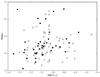 |
Fig. 1 Planetary gravity log (gp) as a function of activity index log ( |
The work of H10 considered different subdatasets by selecting stars and planets that fulfilled the following conditions:
-
1.
Mp > 0.1 MJ, a < 0.1 AU, and 4200 K < Teff < 6200 K;
-
2.
4200 K < Teff < 6200 K;
-
3.
no restrictions,
in which Mp is the mass of the planet, a the semi-major axis of its planetary orbit, and Teff the effective temperature of the star. The constraint on the planetary parameters was used to select only massive close-in planets, and the constraint on effective temperature was used to select only stars for which the log () index had been calibrated (Noyes et al. 1984). The evaluation of these conditions required gathering these quantities from the literature, for which we also used the Exoplanet Encyclopaedia.
When compiling these values, we noted that the Teff values were sometimes different from those used by H10; the difference was occasionally large enough to change the status of a planet-host star relative to the different conditions. To use the most accurate Teff measurements, we therefore reverted to the SWEET-Cat catalog (Santos et al. 2013), an updated catalog of stellar atmospheric parameters for all exoplanet-host stars. The stellar parameters were derived in a homogeneous way for 65% of all planet-hosts and were called baseline parameters. For the remaining 35% of the targets, the parameters were compiled from the literature (and whenever possible from uniform sources). It has been shown that the effective temperature Teff derived by these authors agrees very well with that derived using other standard methods (e.g., the infrared flux method and interferometry) for either the low (Tsantaki et al. 2013) and high temperature range (Sousa et al. 2008). We note that two planets, WASP-69 b and WASP 70 b, are still not listed in SWEET-Cat, but had literature values of 4700 and 5700 K , which means that they satisfy conditions 1 and 2. As before, all the data gathered and their provenance is presented in Appendix A.1.
3. Analysis and results
Our objective is to evaluate the correlation between the quantities log () and log (gp), and to do so, we used the Spearman rank correlation coefficient, as did H10. For each correlation coefficient the p-value was calculated, that is the probability of having a larger or equal correlation coefficient under the hypothesis that the data pairs are uncorrelated (our null hypothesis). To do so, we performed a simple yet reliable nonparametric test: we shuffled the data pairs to create an equivalent uncorrelated dataset (using a Fisher-Yates shuffle to create unbiased datasets), and repeated the experiment 10 000 times. The correlation coefficient of the original dataset was then compared with that of the shuffled population, and the original dataset z-score was calculated. The p-value was then calculated as the one-sided probability of having such a z-score from the observed Gaussian distribution4.
The points selected for each of the conditions described in Sect. 2 and considering Teff from the literature and the SWEET-Cat are plotted in Fig. 2 for the original H10 dataset and the new dataset. The results derived for each of the datasets and each of the conditions are presented in Table 1. We note that these values were not corrected for multiple testing5 and can be directly compared with those of H10. The correction for multiple testing would lead to an increase in p-value, which depends on the estimated number of independent trials done and on the correction method used.
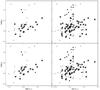 |
Fig. 2 Planetary gravity log (gp) as a function of activity index log ( |
Number of points, Spearman rank correlation coefficient, z-score, and p-value calculated as described in the text.
For the previously published H10 data, we were able to recover very similar values of correlation coefficient and p-value. However, when applying conditions 1 and 2, the correlation coefficient values depended on the source for the effective temperature constraint for the star. The correlation coefficient is highest for condition 1 and lowest for condition 2, for which p-values above 3% cast serious doubts on the presence of the correlation. For the 2014 data, the correlation coefficients are always lower, in the range 0.21−0.47, in contrast with the previous values of 0.29−0.69. With p-values lower than 1%, the correlation seems significant, except for the application of conditions 1 and 2 using literature values for the stellar effective temperature.
In a nutshell, the analysis of data reveals that the correlations are in general still present in the extended 2014 dataset, albeit with lower correlation coefficient values. However, these correlations are not significant for all the conditions tested, depending in particular on the choice of effective temperature constraint.
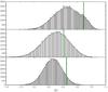 |
Fig. 3 Spearman rank correlation coefficient for a mock population of log ( |
4. Discussion
4.1. Interpretation of the values and validity of the hypothesis
Before we dwell on the interpretation of the results obtained with our extended dataset, it is important to note that the correlation coefficient values obtained from it are systematically lower than those of H10. To understand to which extent these different values are compatible, we estimated the probability of obtaining the correlation coefficients of H10 by a chance draw from our current extended dataset. To do so, we selected from the 2014 dataset 39 random log ()−log (gp) pairs6, the number of datapoints present in H10. We repeated this procedure 10 000 times and compared the distribution obtained with the value originally obtained by H10. After applying it to the whole dataset (i.e., condition 3), we applied the same methodology for the stars selected using conditions 1 and 2; using SWEET-Cat temperatures for this procedure, we selected 19 (or 22) out of the 49 (or 80) pairs available. The results are plotted in Fig. 3. The z-scores of the values using H10 data for the three cases of condition 1, condition 2, and condition 3 (i.e., the whole dataset) were 1.30, 0.27, and 1.52, and assuming a Gaussian distribution they correspond to probabilities of 9.8, 39.5, and 6.4% of having drawn an equal or higher value from the mock pairs distribution. The values obtained for the whole dataset and the stars selected using the different conditions were thus higher than the expected value from the distribution, but the associated probabilities were still high enough to consider it a chance event. We note also that these probabilities do not correspond to independent events and their intersection is not the product of the three, and can be as high as the lowest of the three, 6.4%.
Even though the analysis of H10 is thus compatible with the one presented here, the best estimation of the correlation coefficient is obtained with our extended dataset, with a value significantly lower than presented before. We note that the Spearman rank correlation coefficient provides a measure for the concordance when ordering two variables, to which a p-value must be associated to understand how likely is for the correlation coefficient to arise from a chance event. The correlation coefficient corresponds to the Pearson correlation coefficient of the ranked variables; squaring the correlation coefficient, we obtain the coefficient of determination r2, which we can equate to the explained or shared variance. This means that when we compare the H10 dataset with ours, the shared variance of the ranked variables decreases from 20% to 7%. However, it is important to recall that at this point we are referring to ranked variables, and it is hard to evaluate how this translates into our variable values before the ranking.
An important point to note from Table 1 is the different number of stars selected when applying the different conditions. Since Teff from different sources can vary appreciably, selecting a different Teff origin for the conditions can produce an appreciable difference in the number of stars selected; for instance, for both HAT-P-32 b and WASP-7, the difference is of 200 K. As a consequence, the correlation coefficients change when one uses temperature cutoffs from different sources. Clearly, when the conditions are applied to H10 data, the removal of a single point leads to different correlation coefficients: 0.50 vs. 0.69 for condition 1, and 0.29 vs. 0.41 for condition 2. Interestingly, for both datasets the highest values are obtained for conditions based on SWEET-Cat temperatures. Performing the selection using a more accurate temperature determination will probably lead to a stronger correlation if there is one in the underlying data, and this can be seen as evidence for a correlation. However, this interpretation is complicated by the fact that log () depends on the third power of the (B − V) value of a star, which in turn depends on the Teff (see, e.g., Sousa et al. 2011). This might introduce a concealed bias into the data, and we caution about the limitation of such unguarded interpretations.
A related problem is the validity of the Teff boundaries chosen for the application of the two different criteria. The value of 4200 K is strictly in line with the index calibration limits (Noyes et al. 1984), but it might be over-optimistic given the difficulties at deriving precise parameters, especially for late-K and early-M stars (e.g., Neves et al. 2012; Tsantaki et al. 2013). We note therefore that stars with a temperature similar to the lower limit of the calibration are particularly prone to be misclassified.
Attaching a single activity value to a star is a clear simplification of the problem, because the activity index value of a star varies throughout its activity cycle. As an example, the solar activity index log () ranges from a minimum of −5 to a maximum of −4.75 during its 11 year activity cycle (e.g., Dumusque et al. 2011). Since many of the values reported for log () in our study are obtained from a single observation, we caution that they might not be representative of a given star and a re-observation of these stars at different epochs for coverage of a full activity cycle might ultimately lead to different correlation coefficients. However, given the relatively low scatter expected to be introduced by it, this can not explain the measured index variability. Along the same line, recent studies have demonstrated that a large number of stars have a higher activity level than that of the Sun. For instance, 67−75% of the 150 000 main-sequence stars monitored by the Kepler satellite show a lower activity cycle than our host (Basri et al. 2013). In line with these studies, and as can be seen from Fig. 2, most of the stars in our sample exhibit an activity level below −4.75: 34 of the 49 (69%) selected using condition 1, 61 of the 80 (76%) selected using condition 2, and 85 of the 108 (79%) selected using condition 3 (i.e., the full dataset)7. If one divides each of our samples using this activity cutoff, the lower-activity group still displays significant correlations, while the group composed of more active stars does not, with p-values in excess of 30%, as a consequence of small-number statistics.
Another question is to which extent the radius can be measured accurately for planets orbiting active stars. Some recent studies have shown that such determinations are bound to face some difficulties. The stellar spots that are not occulted during the planetary transit can lead to an overestimation on the planet radius determination of up to 3% Czesla et al. (2009), while the occulted stellar spots during the transit can cause an underestimation on the planet radius determination of up to 4% Oshagh et al. (2013)8. This error on the planet radius could lead to an error of 0.05 on the log (gp) estimation. Since the range of values of log (gp) is wider by more than one order of magnitude than the estimated error, we conclude that the sunspot effect on the planetary density cannot be at the root of the correlation studied in this work.
4.2. Biases of the data and correlation between other variables
An important point already discussed in H10 is that of an observational bias of the sample. This hypothesis was discarded based on the fact that planetary mass and radius (among other parameters) showed a less significant correlation with the activity index. We re-evaluated this point by calculating the correlation between each of these parameters and log () following the procedure described in Sect. 3. For each case we considered the complete dataset and the restricted datasets according to conditions 1 and 2. We present the corresponding results in Table 2. The most significant correlation between the mass and activity index occurs at 0.5% and corresponds to condition 1, while radius and activity do not present a significant correlation for any of the conditions.
Spearman rank correlation coefficient, z-score, and p-value calculated between mass, radius, Teff and log (), as described in the text.
We tried to understand to which extent the measured correlations between mass or radius and the activity indicator could lead to the presented correlation with planetary surface gravity. With this aim we performed a simple test, which is illustrative, without being fully conclusive. We created mock distributions of three variables X, Y, and Z, which represent the activity index, the mass, and the radius, respectively. The activity index distribution X was represented by a standartized Gaussian distribution of N points, while the other two were created by selecting a slope and adding Gaussian noise such that the Spearman rank between ρ(X, Y) and ρ(X, Z) delivered the value of our choice. By this procedure we created sets of three distributions with the same number of points N and correlation coefficients ρ(X, Y) and ρ(X, Z) as delivered in Table 2. We then calculated ρ(X, Y.Z-2), in which the latter distribution is analogous to that of the planetary surface gravity (modulus multiplicative constants, which do not have an impact on the correlation coefficient value). After repeating the experiment 10 000 times, we concluded that the fraction of data sets with a correlation coefficient between our pseudo-surface gravity and pseudo-activity indicators higher than observed were 1% for condition 1 and lower than 0.1% for conditions 2 and 3. Thus, it seems to be very unlikely to draw correlation coefficients as high as in Table 1 starting from correlation coefficients between mass or radius and activity indicators as low as those in Table 2. We stress that this test is more illustrative than definite, because there is a multitude of data pairs and distributions that deliver the same correlation coefficient. However, this simple quantitative analysis is well in line with the discussion of H10, and we have to conclude there is no reason to believe a correlation between the mass and radius and activity indicator could explain the high correlation value between planetary surface gravity and log ().
In addition to these previously explored correlations, we repeated the analysis to explore the correlation between the activity indicator and Teff. We did this using SWEET-Cat temperatures and present the results in Table 2. Very interestingly, effective temperature and log () show a significant anticorrelation with value from 0.37 to 0.51, depending on the condition. Interpreting this correlation, and how it relates with the planetary gravity-activity correlation, is far more complicated. The activity indicator is, by construction, an instrument and effective temperature-independent ratio. The latter property is obtained by dividing the flux at the center of the Ca II line from that on the continuum, and correcting both line and continuum flux for their (B − V) or effective temperature dependence. For more details we refer to Noyes et al. (1984). However, a bias in the calculation between instruments or pipelines might introduce systematic biases in the activity indicator values, which will have an impact on the correlation studied here. For instance, the persistence of a dependence of log () on Teff might lead to a bias of the planetary parameters. In particular, the well-known dependence of the radius anomaly on effective temperature (e.g., Laughlin et al. 2011) and the dependence of planetary mass on stellar mass through the effective temperature (e.g., Lovis & Mayor 2007) could influence the studied correlation. In a similar way to the Teff, which is expected to be an absolute quantity and shows different results reported by different authors, the log () index might show systematic differences that we unfortunately cannot explore by recalculating it in an homogeneous way, because of the unavailability of most of the spectra and the gigantic task implyed by attempting a homogeneous reduction across such a range of instruments and spectra.
Previous works that evaluated the log () distribution for a large number of stars reached different conclusions on the correlation found here. Henry et al. (1996), found no dependence of the activity level on effective temperature (see their Fig. 6 and associated discussion for details), while Lovis et al. (2011) presented opposite evidence from HARPS data. The latter authors noted that log () values for G stars cluster around −5.0, while for K dwarfs they spread over the range from –4.7 to –5.0. The authors then notted that this is in line with a slower decrease of activity with age, as noted by Mamajek & Hillenbrand (2008). The disagreement between studies raises important questions; how a significant correlation can be present in our sample while it is not for other samples is unclear. This can be understood in two ways. First, the correlation between activity and effective temperature might be a consequence of the correlation between activity and planetary surface gravity. The existence of a dependency of activity on effective temperature would introduce a correlation with the latter. Alternatively, the causality might go in the other direction: the correlation between effective temperature and activity might introduce a correlation between surface gravity and activity. This would have to happen through a channel that affects other parameters than planetary mass and planetary radius of the sample; as we saw, the correlation between either of them and activity is very unlikely to account for the high value of planetary surface gravity and activity index. An alternative would be an indirect effect of the planet on the activity level of the star, which would depend on the effective temperature, for instance. This is clearly an extremely involved problem, and to fully address it one should have a homogeneously derived activity indicator sample and preferably a control group of starts without planets at one’s disposal.
The work of H10 already discussed several possible explanations of the correlation; these ranged from environmental effects acting on the planet, such as extreme insolation and evaporation, or feed-back mechanisms into the star resulting from the proximity of the planet, such as enhanced stellar activity. None of these can be confidently refuted, which makes the assessment of the existence of the correlation the more interesting. During the last stage of the refereeing process, we were informed of a contemporary theoretical work that proposes a new explanation for the correlation evaluated here. Lanza (2014) argued that the correlation is due to the absorption by circumstellar material ejected by evaporating planets. Planets with lower atmospheric gravity have a greater mass-loss and are thus associated with a higher column density of circumstellar absorption, which in turn leads to a lower level of chromospheric emission as is observed by us.
We would like to conclude this section with a note to the ongoing existing transiting-planet follow-up campaigns: we encourage the publication of log () values instead of S index values. In this way, the activity can be compared between stars and instruments, and more general trends such as those discussed here can emerge. We also encourage the presentation of upper limits in the case of a nondetection of Ca II emission, so that a tobit-like analysis (e.g., Figueira et al. 2014) can be performed.
5. Conclusions
We presented an updated analysis on the correlation between stellar host activity as measured by the index log () and orbiting planetary surface gravity. An updated dataset roughly three times larger than the original one shows significant correlation as delivered by the Spearman rank correlation coefficient, but with lower coefficient values. These values are compatible with those of H10 when considering small-number statistics on the current data, showing that the two datasets are not significantly different.
The correlation is recovered for star-planet pairs selected using the different conditions proposed by H10. Remarkably, using the more homogeneous and accurate SWEET-Cat temperatures led to higher correlation coefficient values. This can be interpreted as evidence for the existence of a real correlation in the data, but more complex dependencies might lurk within as a result of the dependence of the activity index on the effective temperature, of which we highlighted importance and relation to the surface gravity-activity index correlation.
Several additional effects on top of those discussed by H10 were considered, but none fully explains the detected correlation. The very recent and contemporary work of Lanza (2014) provides the best explanation to date. In light of the complex question discussed here, we encourage the different follow-up teams to publish their activity index values in the form of log () index so that a comparison between stars and instruments can be made.
Online material
Appendix A: Literature data
To perform this study we gathered the data as described in Sect. 2. The data employed are present in the table below.
Parameters for each star-planet pair and their provenance.
As of 07/07/2014.
We note that we could have started our analysis from the Exoplanet Orbit Database, but the number of planets and transiting planets listed on both sites showed that the Exoplanet Encyclopaedia was more comprehensive.
A notable exception was the recent work of Marcy et al. (2014), which provided the activity index values for each observation. In this case we used the average value as representative of each star.
For more on this method and a python implementation of it the reader is referred to Figueira et al. (2013); Santos et al. (2014).
See, for instance, http://en.wikipedia.org/wiki/Multiple_comparisons_problem.
By “random” we mean that the pair chosen was random, but there was no shuffling or re-pairing of variables.
We note, however, that the detected planets are affected by selection bias, and their host properties might not reflect those of stars in the solar neighborhood.
Note that the upper limit on the underestimation or overestimation on the planet radius estimation was obtained for the highest sunspot filling factor, as measured during the maximum activity phase of the solar cycle.
Acknowledgments
This work was supported by the European Research Council/European Community under the FP7 through Starting Grant agreement number 239953. P.F. and N.C.S. acknowledge support by Fundação para a Ciência e a Tecnologia (FCT) through Investigador FCT contracts of reference IF/01037/2013 and IF/00169/2012, respectively, and POPH/FSE (EC) by FEDER funding through the program “Programa Operacional de Factores de Competitividade - COMPETE”. VZhA and MO acknowledge the support from the Fundação para a Ciência e Tecnologia, FCT (Portugal) in the form of the fellowships of reference SFRH/BPD/70574/2010 and SFRH/BD/51981/2012, respectively, from the FCT (Portugal). PF thanks Christophe Lovis and Maxime Marmier for a helpful discussion on the activity index definition, and Paulo Peixoto for the very hepful support on IT issues. We are indebted to the anonymous referee for constructive and insightful comments. We warmly thank all those who develop the Python language and its scientific packages and keep them alive and free. This research has made use of the Exoplanet Orbit Database and the Exoplanet Data Explorer at exoplanets.org.
References
- Albrecht, S., Winn, J. N., Butler, R. P., et al. 2012, ApJ, 744, 189 [NASA ADS] [CrossRef] [Google Scholar]
- Anderson, D. R., Collier Cameron, A., Gillon, M., et al. 2011, A&A, 534, A16 [NASA ADS] [CrossRef] [EDP Sciences] [Google Scholar]
- Anderson, D. R., Collier Cameron, A., Delrez, L., et al. 2014, MNRAS, 445, 1114 [NASA ADS] [CrossRef] [Google Scholar]
- Bakos, G. Á., Hartman, J. D., Torres, G., et al. 2012, AJ, 144, 19 [NASA ADS] [CrossRef] [Google Scholar]
- Ballard, S., Fabrycky, D., Fressin, F., et al. 2011, ApJ, 743, 200 [NASA ADS] [CrossRef] [Google Scholar]
- Basri, G., Walkowicz, L. M., & Reiners, A. 2013, ApJ, 769, 37 [NASA ADS] [CrossRef] [Google Scholar]
- Beerer, I. M., Knutson, H. A., Burrows, A., et al. 2011, ApJ, 727, 23 [NASA ADS] [CrossRef] [Google Scholar]
- Béky, B., Bakos, G. Á., Hartman, J., et al. 2011, ApJ, 734, 109 [NASA ADS] [CrossRef] [Google Scholar]
- Bonfils, X., Delfosse, X., Udry, S., et al. 2013, A&A, 549, A109 [NASA ADS] [CrossRef] [EDP Sciences] [Google Scholar]
- Borucki, W. J., Koch, D. G., Basri, G., et al. 2011, ApJ, 736, 19 [NASA ADS] [CrossRef] [Google Scholar]
- Borucki, W. J., Agol, E., Fressin, F., et al. 2013, Science, 340, 587 [NASA ADS] [CrossRef] [PubMed] [Google Scholar]
- Boué, G., Figueira, P., Correia, A. C. M., & Santos, N. C. 2012, A&A, 537, L3 [NASA ADS] [CrossRef] [EDP Sciences] [Google Scholar]
- Brown, D. J. A., Cameron, A. C., Anderson, D. R., et al. 2012, MNRAS, 423, 1503 [NASA ADS] [CrossRef] [Google Scholar]
- Buchhave, L. A., Bakos, G. Á., Hartman, J. D., et al. 2010, ApJ, 720, 1118 [NASA ADS] [CrossRef] [Google Scholar]
- Buchhave, L. A., Bakos, G. Á., Hartman, J. D., et al. 2011, ApJ, 733, 116 [NASA ADS] [CrossRef] [Google Scholar]
- Covino, E., Esposito, M., Barbieri, M., et al. 2013, A&A, 554, A28 [NASA ADS] [CrossRef] [EDP Sciences] [Google Scholar]
- Czesla, S., Huber, K. F., Wolter, U., Schröter, S., & Schmitt, J. H. M. M. 2009, A&A, 505, 1277 [NASA ADS] [CrossRef] [EDP Sciences] [Google Scholar]
- Dressing, C. D., & Charbonneau, D. 2013, ApJ, 767, 95 [NASA ADS] [CrossRef] [Google Scholar]
- Dumusque, X., Santos, N. C., Udry, S., Lovis, C., & Bonfils, X. 2011, A&A, 527, A82 [NASA ADS] [CrossRef] [EDP Sciences] [Google Scholar]
- Dumusque, X., Bonomo, A. S., Haywood, R. D., et al. 2014, ApJ, 789, 154 [NASA ADS] [CrossRef] [Google Scholar]
- Figueira, P., Marmier, M., Boué, G., et al. 2012, A&A, 541, A139 [NASA ADS] [CrossRef] [EDP Sciences] [Google Scholar]
- Figueira, P., Santos, N. C., Pepe, F., Lovis, C., & Nardetto, N. 2013, A&A, 557, A93 [NASA ADS] [CrossRef] [EDP Sciences] [Google Scholar]
- Figueira, P., Faria, J. P., Delgado-Mena, E., et al. 2014, A&A, 570, A21 [NASA ADS] [CrossRef] [EDP Sciences] [Google Scholar]
- Gautier, III, T. N., Charbonneau, D., Rowe, J. F., et al. 2012, ApJ, 749, 15 [NASA ADS] [CrossRef] [Google Scholar]
- Gilliland, R. L., Marcy, G. W., Rowe, J. F., et al. 2013, ApJ, 766, 40 [NASA ADS] [CrossRef] [Google Scholar]
- Gillon, M., Doyle, A. P., Lendl, M., et al. 2011, A&A, 533, A88 [NASA ADS] [CrossRef] [EDP Sciences] [Google Scholar]
- Hartman, J. D. 2010, ApJ, 717, L138 [NASA ADS] [CrossRef] [Google Scholar]
- Hartman, J. D., Bakos, G. Á., Kipping, D. M., et al. 2011a, ApJ, 728, 138 [NASA ADS] [CrossRef] [Google Scholar]
- Hartman, J. D., Bakos, G. Á., Torres, G., et al. 2011b, ApJ, 742, 59 [NASA ADS] [CrossRef] [Google Scholar]
- Hartman, J. D., Bakos, G. Á., Béky, B., et al. 2012, AJ, 144, 139 [NASA ADS] [CrossRef] [Google Scholar]
- Hartman, J. D., Bakos, G. Á., Torres, G., et al. 2014, AJ, 147, 128 [NASA ADS] [CrossRef] [Google Scholar]
- Hébrard, G., Collier Cameron, A., Brown, D. J. A., et al. 2013, A&A, 549, A134 [NASA ADS] [CrossRef] [EDP Sciences] [Google Scholar]
- Henry, T. J., Soderblom, D. R., Donahue, R. A., & Baliunas, S. L. 1996, AJ, 111, 439 [NASA ADS] [CrossRef] [Google Scholar]
- Howard, A. W., Johnson, J. A., Marcy, G. W., et al. 2011, ApJ, 730, 10 [NASA ADS] [CrossRef] [Google Scholar]
- Howard, A. W., Bakos, G. Á., Hartman, J., et al. 2012a, ApJ, 749, 134 [NASA ADS] [CrossRef] [Google Scholar]
- Howard, A. W., Marcy, G. W., Bryson, S. T., et al. 2012b, ApJS, 201, 15 [NASA ADS] [CrossRef] [Google Scholar]
- Kipping, D. M., Hartman, J., Bakos, G. Á., et al. 2011, AJ, 142, 95 [NASA ADS] [CrossRef] [Google Scholar]
- Knutson, H. A., Howard, A. W., & Isaacson, H. 2010, ApJ, 720, 1569 [NASA ADS] [CrossRef] [Google Scholar]
- Kovács, G., Bakos, G. Á., Hartman, J. D., et al. 2010, ApJ, 724, 866 [NASA ADS] [CrossRef] [Google Scholar]
- Lanza, A. F. 2014, A&A, 572, L6 [NASA ADS] [CrossRef] [EDP Sciences] [Google Scholar]
- Laughlin, G., Crismani, M., & Adams, F. C. 2011, ApJ, 729, L7 [NASA ADS] [CrossRef] [Google Scholar]
- Lecavelier Des Etangs, A., Ehrenreich, D., Vidal-Madjar, A., et al. 2010, A&A, 514, A72 [NASA ADS] [CrossRef] [EDP Sciences] [Google Scholar]
- Lendl, M., Anderson, D. R., Collier-Cameron, A., et al. 2012, A&A, 544, A72 [NASA ADS] [CrossRef] [EDP Sciences] [Google Scholar]
- Lendl, M., Triaud, A. H. M. J., Anderson, D. R., et al. 2014, A&A, 568, A81 [NASA ADS] [CrossRef] [EDP Sciences] [Google Scholar]
- Lovis, C., & Mayor, M. 2007, A&A, 472, 657 [NASA ADS] [CrossRef] [EDP Sciences] [Google Scholar]
- Lovis, C., Dumusque, X., Santos, N. C., et al. 2011, A&A, submitted [arXiv:1107.5325] [Google Scholar]
- Mamajek, E. E., & Hillenbrand, L. A. 2008, ApJ, 687, 1264 [NASA ADS] [CrossRef] [Google Scholar]
- Mancini, L., Southworth, J., Ciceri, S., et al. 2014, A&A, 562, A126 [NASA ADS] [CrossRef] [EDP Sciences] [Google Scholar]
- Marcy, G. W., Isaacson, H., Howard, A. W., et al. 2014, ApJS, 210, 20 [NASA ADS] [CrossRef] [Google Scholar]
- Marmier, M., Ségransan, D., Udry, S., et al. 2013, A&A, 551, A90 [NASA ADS] [CrossRef] [EDP Sciences] [Google Scholar]
- Maxted, P. F. L., Anderson, D. R., Collier Cameron, A., et al. 2011, PASP, 123, 547 [NASA ADS] [CrossRef] [Google Scholar]
- Mayor, M., Marmier, M., Lovis, C., et al. 2011, A&A, submitted [arXiv:1109.2497] [Google Scholar]
- McArthur, B. E., Endl, M., Cochran, W. D., et al. 2004, ApJ, 614, L81 [NASA ADS] [CrossRef] [Google Scholar]
- Neves, V., Bonfils, X., Santos, N. C., et al. 2012, A&A, 538, A25 [NASA ADS] [CrossRef] [EDP Sciences] [Google Scholar]
- Noyes, R. W., Hartmann, L. W., Baliunas, S. L., Duncan, D. K., & Vaughan, A. H. 1984, ApJ, 279, 763 [NASA ADS] [CrossRef] [Google Scholar]
- O’Rourke, J. G., Knutson, H. A., Zhao, M., et al. 2014, ApJ, 781, 109 [NASA ADS] [CrossRef] [Google Scholar]
- Oshagh, M., Santos, N. C., Boisse, I., et al. 2013, A&A, 556, A19 [NASA ADS] [CrossRef] [EDP Sciences] [Google Scholar]
- Pepe, F., Cameron, A. C., Latham, D. W., et al. 2013, Nature, 503, 377 [NASA ADS] [CrossRef] [PubMed] [Google Scholar]
- Poppenhaeger, K., & Wolk, S. J. 2014, A&A, 565, L1 [NASA ADS] [CrossRef] [EDP Sciences] [Google Scholar]
- Poppenhaeger, K., Lenz, L. F., Reiners, A., Schmitt, J. H. M. M., & Shkolnik, E. 2011, A&A, 528, A58 [NASA ADS] [CrossRef] [EDP Sciences] [Google Scholar]
- Queloz, D., Bouchy, F., Moutou, C., et al. 2009, A&A, 506, 303 [NASA ADS] [CrossRef] [EDP Sciences] [Google Scholar]
- Quinn, S. N., Bakos, G. Á., Hartman, J., et al. 2012, ApJ, 745, 80 [NASA ADS] [CrossRef] [Google Scholar]
- Saar, S. H., & Cuntz, M. 2001, MNRAS, 325, 55 [NASA ADS] [CrossRef] [Google Scholar]
- Santos, N. C., Sousa, S. G., Mortier, A., et al. 2013, A&A, 556, A150 [NASA ADS] [CrossRef] [EDP Sciences] [Google Scholar]
- Santos, N. C., Mortier, A., Faria, J. P., et al. 2014, A&A, 566, A35 [NASA ADS] [CrossRef] [EDP Sciences] [Google Scholar]
- Sato, B., Hartman, J. D., Bakos, G. Á., et al. 2012, PASJ, 64, 97 [NASA ADS] [Google Scholar]
- Schneider, J., Dedieu, C., Le Sidaner, P., Savalle, R., & Zolotukhin, I. 2011, A&A, 532, A79 [NASA ADS] [CrossRef] [EDP Sciences] [Google Scholar]
- Shkolnik, E., Bohlender, D. A., Walker, G. A. H., & Collier Cameron, A. 2008, ApJ, 676, 628 [NASA ADS] [CrossRef] [Google Scholar]
- Silburt, A., Gaidos, E., & Wu, Y. 2014 [arXiv:1406.6048] [Google Scholar]
- Sousa, S. G., Santos, N. C., Mayor, M., et al. 2008, A&A, 487, 373 [NASA ADS] [CrossRef] [EDP Sciences] [MathSciNet] [Google Scholar]
- Sousa, S. G., Santos, N. C., Israelian, G., et al. 2011, A&A, 526, A99 [NASA ADS] [CrossRef] [EDP Sciences] [Google Scholar]
- Southworth, J., Wheatley, P. J., & Sams, G. 2007, MNRAS, 379, L11 [NASA ADS] [CrossRef] [Google Scholar]
- Triaud, A. H. M. J., Collier Cameron, A., Queloz, D., et al. 2010, A&A, 524, A25 [NASA ADS] [CrossRef] [EDP Sciences] [Google Scholar]
- Triaud, A. H. M. J., Queloz, D., Hellier, C., et al. 2011, A&A, 531, A24 [NASA ADS] [CrossRef] [EDP Sciences] [Google Scholar]
- Tsantaki, M., Sousa, S. G., Adibekyan, V. Z., et al. 2013, A&A, 555, A150 [NASA ADS] [CrossRef] [EDP Sciences] [Google Scholar]
- Udry, S., & Santos, N. C. 2007, ARA&A, 45, 397 [NASA ADS] [CrossRef] [Google Scholar]
- Winn, J. N., Albrecht, S., Johnson, J. A., et al. 2011, ApJ, 741, L1 [NASA ADS] [CrossRef] [Google Scholar]
- Wright, J. T., Fakhouri, O., Marcy, G. W., et al. 2011, PASP, 123, 412 [NASA ADS] [CrossRef] [Google Scholar]
All Tables
Number of points, Spearman rank correlation coefficient, z-score, and p-value calculated as described in the text.
Spearman rank correlation coefficient, z-score, and p-value calculated between mass, radius, Teff and log (), as described in the text.
All Figures
|
Fig. 1 Planetary gravity log (gp) as a function of activity index log ( |
| In the text | |
|
Fig. 2 Planetary gravity log (gp) as a function of activity index log ( |
| In the text | |
|
Fig. 3 Spearman rank correlation coefficient for a mock population of log ( |
| In the text | |
Current usage metrics show cumulative count of Article Views (full-text article views including HTML views, PDF and ePub downloads, according to the available data) and Abstracts Views on Vision4Press platform.
Data correspond to usage on the plateform after 2015. The current usage metrics is available 48-96 hours after online publication and is updated daily on week days.
Initial download of the metrics may take a while.