| Issue |
A&A
Volume 572, December 2014
|
|
|---|---|---|
| Article Number | A68 | |
| Number of page(s) | 12 | |
| Section | Extragalactic astronomy | |
| DOI | https://doi.org/10.1051/0004-6361/201424677 | |
| Published online | 01 December 2014 | |
Are compact groups hostile towards faint galaxies?⋆
1
Instituto de Astronomía Teórica y Experimental, IATE,
5000 CONICET
5000
Córdoba
Argentina
e-mail:
This email address is being protected from spambots. You need JavaScript enabled to view it.
2
Observatorio Astronómico, Universidad Nacional de
Córdoba, Laprida 854,
X5000BGR
5000
Córdoba,
Argentina
3
Instituto de Astronomía, Geofísica e Ciencias Atmosfericas, IAG, USP, Rua do Matão
1226, 05508-090
São Paulo,
Brazil
Received: 24 July 2014
Accepted: 23 September 2014
Abstract
Aims. The goal of this work is to understand whether the extreme environment of compact groups (CGs) can affect the distribution and abundance of faint galaxies around them.
Methods. We performed an analysis of the faint galaxy population in the vicinity of compact and normal groups. We built a light-cone mock galaxy catalogue constructed from the Millennium Run Simulation II plus a semi-analytical model of galaxy formation. We identified a sample of CGs in the mock catalogue as well as a control sample of normal galaxy groups and computed the projected number density profiles of faint galaxies around the first and the second ranked galaxies. We also compared the profiles obtained from the semi-analytical galaxies in CGs with those obtained from observational data. In addition, we investigated whether the ranking or the luminosity of a galaxy is the most important parameter in the determination of the centre around which the clustering of faint galaxies occurs.
Results. There is no particular influence of the extreme compact group (CG) environment on the number of faint galaxies in such groups compared to control groups. When selecting normal groups with separations between the first and second ranked galaxies similar to what is observed in CGs, the faint galaxy projected number density profiles in CGs and normal groups are similar in shape and height. We observed a similar behaviour of the population of faint galaxies in observations and simulations in the regions closer to the first and second ranked galaxies. Finally, we find that the projected density of faint galaxies is higher around luminous galaxies, regardless of the ranking in the CG.
Conclusions. The semi-analytical approach shows that CGs and their surroundings do not represent a hostile enough environment to make faint galaxies behave differently than in normal groups.
Key words: methods: numerical / methods: statistical / galaxies: groups: general
Appendix A is available in electronic form at http://www.aanda.org
© ESO, 2014
1. Introduction
Overdense regions in the universe are the most natural laboratories in which to witness galaxy formation and evolution. Among them, the most extreme environment in the universe can be found by analysing compact groups (CGs) of galaxies. These small systems of a few galaxies in close proximity represent an important element in extragalactic astronomy for the study of galaxy interactions and to investigate how they lead to the morphological transformation of the member galaxies through the lifetime of the group.
Since the construction of the first catalogues of CGs by visual inspection (Rose 1977; Hickson 1982), several studies have been performed analysing these groups and their galaxy members. Some of these studies have addressed topics such as internal structures, morphologies, luminosities, and environments (e.g. Hickson et al. 1984; Mamon 1986; Hickson & Rood 1988; Mendes de Oliveira & Hickson 1991; Prandoni et al. 1994; Kelm & Focardi 2004) an attempt to unveil their formation scenario. Over the years, evidence has been gathered to clarify whether they are recently formed systems that are about to coalesce into a single galaxy (Hickson & Rood 1988), or transient unbound cores of looser groups (Tovmassian et al. 2001), or just simple chance alignments of galaxies along the line of sight within larger systems (Walke & Mamon 1989; Hernquist et al. 1995).
Since most of the famous CGs were identified relying on a visual inspection (following the Hickson selection criterion; Hickson 1982), understanding the intrinsic nature of CGs has always been challenging, prompting scientist to perform different kinds of numerical tests to quantify their reliability. Among these tests, the studies performed using numerical simulations plus semi-analytic models have proven to be a very important tool to improve our understanding of these groups (McConnachie et al. 2008; Díaz-Giménez & Mamon 2010). For instance, such studies confirm that roughly 70 per cent of CGs identified using Hickson’s criterion can be considered physically dense groups and that the Hickson sample is incomplete (Díaz-Giménez & Mamon 2010).
Even though many efforts have been devoted to studying CGs, their members, and the signs of interaction as a way to understand all the relevant processes involved in galaxy evolution, most of them have overlooked the impact of these extremely dense regions on numbers and distributions of the faint galaxies. These galaxies are a very important population in galaxy systems (e.g. González et al. 2006), and given the high density and the low velocity dispersion of CGs, they are very suitable for analysing the effects of interaction-inductive environments on the faint galaxy structure and evolution. It is usually expected that such dense environment of CGs can drastically affect the evolution of their brightest members, but are these environments hostile enough to alter the faint galaxy population distribution as well? Performing such studies using observations is done less often for two different reasons: first, by definition of CGs, galaxies are considered as members of these systems only if their magnitudes are within a three-magnitude range from the brightest member, therefore fainter galaxies are just ignored in the samples; second, it could be difficult to detect these faint objects and actually very few studies have been carried out analysing this population in individual CGs (e.g. Ribeiro et al. 1994; Zabludoff & Mulchaey 1998; Amram et al. 2004; Campos et al. 2004; Carrasco et al. 2006; Krusch et al. 2006; Da Rocha et al. 2011; Konstantopoulos et al. 2013). Hence, more evidence is needed to understand the relevance of this particular environment on faint galaxies in/around CGs.
Given that these types of studies require the use of catalogues which contain a large population of faint galaxies as well as spectroscopic information to ensure proximity to the environment of CGs, the best way to approach the problem is to perform this analysis using synthetic catalogues constructed from numerical simulations plus semi-analytic models of galaxy formation. Recently, a high resolution N-body numerical simulation was released, the Millennium Run Simulation II (Boylan-Kolchin et al. 2009), perfect for resolving dwarf galaxies using semi-analytic recipes. A particular set of recipes was already applied to this simulation, (Guo et al. 2011), producing a very suitable sample of synthetic galaxies that has been made available for the astronomical community. The semi-analytic model has been tuned to reproduce the z = 0 stellar mass function and luminosity function, making it a suitable tool with which to understand the evolution of faint galaxies. Therefore, in this work we will use this available tool to study, from the semi-analytical point of view, whether the population of faint galaxies in/around CGs is affected by the environment of these systems.
The layout of this paper is as follows: in Sect. 2, we describe the N-body simulation and the semi-analytic model of galaxy formation used to build the mock catalogue. In Sect. 3 we describe the different procedures adopted for the CG identification as well as the construction of a control sample of normal groups. In Sect. 4 we construct the sample of faint galaxies around the galaxy systems and compute the projected number density profiles taking into account the properties of faint galaxies and those of the CGs they inhabit. In Sect. 5 we perform a comparison between the projected number density profiles obtained from mock catalogues with those obtained for a sample of CGs identified from observations. Finally, in Sect. 6 we summarise our results.
2. The mock galaxy catalogue
We built a light-cone mock catalogue using a simulated set of galaxies extracted from the Guo et al. (2011) semi-analytic model of galaxy formation applied on top of the Millennium Run Simulation II (Boylan-Kolchin et al. 2009).
2.1. The N-body simulation
The Millennium Run Simulation II is a cosmological tree-particle-mesh (Xu 1995) N-body Simulation, which evolves 10 billion (21603) dark matter particles in a 100 h-1 Mpc periodic box, using a comoving softening length of 1 h-1 kpc (Boylan-Kolchin et al. 2009). The cosmological parameters of this simulation are consistent with WMAP1 data (Spergel et al. 2003), i.e. a flat cosmological model with a non-vanishing cosmological constant (ΛCDM): Ωm = 0.25, Ωb = 0.045, ΩΛ = 0.75, σ8 = 0.9, n=1, and h = 0.73. The simulation was started at z = 127, with the particles initially positioned in a glass-like distribution according to the ΛCDM primordial density fluctuation power spectrum. The mass resolution is 125 times better than that obtained in the Millennium Run Simulation I (Springel et al. 2005), i.e. each particle of mass has 6.9 × 10⁶h-1M⊙. With this resolution, halos of typical dwarf spheroids are resolved and halos similar to the mass of our Milky Way have hundreds of thousands of particles (Boylan-Kolchin et al. 2009).
It is well known that WMAP7 (Komatsu et al. 2011) yielded different cosmological parameters than the ones used here (from WMAP1). Therefore, one may argue that the studies carried out in the present simulation could produce results that do not agree with the current cosmological model. However, Guo et al. (2013) have demonstrated that the abundance and clustering of dark halos and galaxy properties, including clustering, in WMAP7 are very similar to those found in WMAP1 for z ≤ 3, which is far inside the redshift range of interest in this work (see Sect. 2.3).
2.2. The semi-analytic model
To obtain a simulated galaxy set we adopted the Guo et al. (2011) semi-analytic model. This particular model fixed several open issues present in some of its predecessors, such as the efficiency of supernova feedback and the fit of the stellar mass function of galaxies at low redshifts. Guo et al. (2011) also introduced a more realistic treatment of satellite galaxy evolution and of mergers, allowing satellites to continue forming stars for a longer period of time and reducing the excessively rapid reddening of the satellite. The model also includes a treatment of the tidal disruption of satellite galaxies. Compared to previous versions of the semi-analytical models, the Guo et al. model has a lower number of galaxies than its predecessors, at any redshift and in any environment. This is the result of a stronger stellar feedback that reduces the number of low-mass galaxies, and a model of stellar stripping, which contributes to reducing the number of intermediate to low mass galaxies (Vulcani et al. 2014).
This model produces a complete sample when considering galaxies with stellar masses larger than ~106.4h-1M⊙. This implies that the galaxy sample is almost complete down to an absolute magnitude in the rSDSS-band of −11.
2.3. Mock catalogue construction
To construct a mock galaxy catalogue we followed a similar procedure to that described in Zandivarez et al. (2014). The procedure is as follows:
-
We locate a virtual observer at zero redshift and find the galaxies that lie on the observer’s backward light-cone. The catalogue is constructed by adding shells taken from different snapshots corresponding to the epoch of the lookback time at their corresponding distance (Díaz-Giménez 2002; Henriques et al. 2012; Wang & White 2012).
-
Given the requirements of our work with CGs, we introduce a maximum redshift of 0.5.
-
Because of the limited size of the simulation box, 100 h-1 Mpc, we use the periodicity of the box and build a super-box to reach the desired maximum distance.
-
The cosmological redshift (zc) is obtained from the comoving distance of the galaxies in the super-box and the distorted or spectroscopic redshift (zs) is computed considering the peculiar velocities of the galaxies in the radial direction (vp), i.e. zs = (1 + zc)(1 + vp/ c) − 1, where c is the velocity of the light.
-
To avoid discreteness of the galaxy magnitudes due to the size of the shells, we interpolate the absolute magnitudes among two consecutive shells, according to their distance to the shell edges.
-
We use the prescription of Zandivarez et al. (2014) to avoid the problems of repeated or missing galaxies in the boundaries of two consecutive shells due to the proper movements of the galaxies from one snapshot to the next.
-
We compute k-corrections for each galaxy using an iterative procedure based on the prescriptions given by Chilingarian et al. (2010).
The final mock catalogue comprises 775439 galaxies down to an apparent magnitude limit rlim = 16.3 within a solid angle of 4π. We also selected a sample of galaxies within the same volume, but having apparent magnitude limit of 21, which will be used to select the faint neighbours. This new sample has ~140 million galaxies.
3. Selecting the samples of groups
3.1. Compact group sample
We defined a mock velocity-filtered CG sample following the prescriptions of Díaz-Giménez & Mamon (2010) and Díaz-Giménez et al. (2012). Briefly, the automated searching algorithm defines as CGs those that satisfy the criteria
-
4 ≤ N ≤ 10 (population),
-
μr ≤ 26.33 mag arcsec-2 (compactness),
-
ΘN> 3ΘG (isolation),
-
rbrightest ≤ rlim − 3 = 13.3 (flux limit),
-
| vi − ⟨ v ⟩ | ≤ 1000 km s-1 (velocity filtering),
where N is the total number of galaxies whose r-band magnitude satisfies r<rbrightest + 3, and rbrightest is the apparent magnitude of the brightest galaxy of the group; μr is the mean r-band surface brightness, averaged over the smallest circle circumscribing the galaxy centres; ΘG is the angular diameter of the smallest circumscribed circle; ΘN is the angular diameter of the largest concentric circle that contains no other galaxies within the considered magnitude range or brighter; vi is the radial velocity of each galaxy member; and ⟨ v ⟩ is the median of the radial velocity of the members. The compactness and flux limit criteria are set to match the identification in the 2MASS catalogue performed in Díaz-Giménez et al. (2012).
As in previous works, we have considered that mock galaxies that are close in projection on the plane of the mock sky would be blended by observers if their angular separation is less than the sum of their angular half-light radii. Therefore, only groups with more than four members after blending galaxies survive.
This algorithm identifies 431 CGs.
3.2. Control group sample
To build a group sample to compare the results obtained for CGs, we identified galaxy groups in the same mock galaxy catalogue. The identification was performed using a friends-of-friends (FoF) algorithm similar to that developed by Huchra & Geller (1982) to identify galaxy systems in redshift space for a flux-limited catalogue. The algorithm links galaxies that share common neighbours, i.e. pairs of galaxies with projected separations smaller than D0 and radial velocity differences less than V0. Following the prescriptions of Zandivarez et al. (2014), we used a radial linking length of V0 = 130 km s-1 and a transversal linking length, D0, defined by a contour overdensity contrast of δρ/ρ = 433 (see Eq. (4) in Huchra & Geller 1982). This value of δρ/ρ is adopted since it is expected that galaxies are more concentrated than dark matter (Eke et al. 2004; Berlind et al. 2006); therefore we should use a higher density contrast than that usually adopted in dark matter simulations, between 150−200 (see Appendix B of Zandivarez et al. 2014; for details).
Since we are dealing with a flux limited sample of galaxies, both linking lengths have to be weighted by a factor, R, to take into account the variation of the sampling of the luminosity function produced by the different distances of the groups to the observers. Factor R was proposed by Huchra & Geller (1982) and is computed using the galaxy luminosity function following the equation ![Mathematical equation: \begin{eqnarray*} R=\left[ \frac{\int_{-\infty}^{M_{12}} \phi(M) {\rm d}M}{\int_{-\infty}^{M_{\rm lim}} \phi(M) {\rm d}M} \right]^{-1/3}, \end{eqnarray*}](/articles/aa/full_html/2014/12/aa24677-14/aa24677-14-eq53.png) where Mlim = −13.7, and M12 = rlim − 25−5log (dL12) with dL12 the mean luminosity distance for the galaxy pair. Therefore, we used the information from the semi-analytic model to compute the luminosity function for the z = 0 snapshot of the simulation. Using a Levenberg-Marquardt method, we fitted a double-Schechter function to the distribution of rest frame rSDSS absolute magnitudes,
where Mlim = −13.7, and M12 = rlim − 25−5log (dL12) with dL12 the mean luminosity distance for the galaxy pair. Therefore, we used the information from the semi-analytic model to compute the luminosity function for the z = 0 snapshot of the simulation. Using a Levenberg-Marquardt method, we fitted a double-Schechter function to the distribution of rest frame rSDSS absolute magnitudes, ![Mathematical equation: \begin{eqnarray*} \phi(L)=\frac{1}{L^{\ast}}\exp\left( -\frac{L}{L^{\ast}} \right) \left[ \phi_1 \left( \frac{L}{L^{\ast}} \right)^{\alpha_1} + \phi_2 \left( \frac{L}{L^{\ast}} \right)^{\alpha_2} \right], \end{eqnarray*}](/articles/aa/full_html/2014/12/aa24677-14/aa24677-14-eq57.png) obtaining as best fitted parameters: M∗ − 5log (h) = −20.3 ± 0.1, φ1 = 0.0156 ± 0.0003, α1 = −0.06 ± 0.02, φ2 = 0.0062 ± 0.0003, and α2 = −1.41 ± 0.02.
obtaining as best fitted parameters: M∗ − 5log (h) = −20.3 ± 0.1, φ1 = 0.0156 ± 0.0003, α1 = −0.06 ± 0.02, φ2 = 0.0062 ± 0.0003, and α2 = −1.41 ± 0.02.
Using the all-sky mock catalogue, this algorithm produced a sample of 1897 groups with 10 or more galaxy members with magnitudes brighter than rSDSS-band of 16.3 and up to redshift 0.1
We imposed the following constraints on the identified group sample to select the sample of control groups:
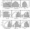 |
Fig. 1 Distributions of observable properties of compact and control groups. Number of members in a three-magnitude range (top-left panel), radial velocity of the groups (top-centre panel), rest frame r-band absolute magnitude of the brightest galaxy member (top-right panel), difference in absolute magnitude between the brightest and the 2nd brightest galaxy of the groups (middle-left panel), projected radius of the minimum circle that encloses the galaxy members (middle-centre panel), projected distance between the brightest and 2nd brightest galaxies (middle-right panel), mean group surface brightness (bottom-left panel), radial velocity dispersion of the groups (bottom-centre panel), and dimensionless crossing time (bottom-right panel). Black empty histograms correspond to CGs (CGs), while grey histograms correspond to control groups (S1). Error bars correspond to Poisson errors. |
-
rbrightest< 13.3. This limit was imposed to match the flux limit criterion in the identification of CGs. This restriction ensures that all the groups have the same chance of including all the existing galaxies within a three-magnitude range from the brightest. The sample that remains comprises 741 galaxy groups.
-
 , where (
 ) is the number of members in a three-magnitude range from the brightest. This constraint was included to mimic the galaxy population allowed in the CGs sample. This limit restrict the group sample to 315 systems.
 -
We also discarded those galaxy groups that share galaxies with the CGs of our sample. The remaining sample comprises 231 galaxy groups.
-
Finally, we excluded from our control group sample those with a bright galaxy (brighter than the brightest galaxy of the FoF group) inside the cylinder used to compute the projected density profiles (see next section for further details about the cylinder definition). This restriction produces a final control group sample of 108 galaxy groups.
The sample of control groups is referred to as the S1 sample in the figures that follow. It is worth mentioning that the different algorithms used to identify the CGs and control groups mean that the two samples do not completely overlap, i.e. not all CGs meet the requirements for inclusion in the sample of control groups (prior to the exclusion of groups that are in the CG sample, obviously), and vice versa.
In Fig. 1 we show a comparison between the observable group properties of the CG sample (black empty histograms) and the S1 sample (grey histograms). All the properties have been computed using only the members within a three magnitude range from the brightest galaxy. We show properties that are commonly derived when studying CGs, although some of them are barely defined for normal groups (e.g. the radius of the minimum circle that encloses all the galaxy members). From this comparison, it can be seen that both samples span similar ranges of distances, magnitudes of the brightest galaxy, and radial velocity dispersions. As expected, normal groups show larger membership, projected size, and projected separation between their two brightest galaxies, and fainter surface brightness. They also show larger crossing times, computed as  where ⟨ dij ⟩ is the median of the inter-galaxy projected separations in h-1 Mpc.
4. Projected density profiles of faint galaxies
4.1. Faint galaxies in/around groups
We consider as faint galaxies those galaxies that were not included as group members given the population criterion considered by Hickson, but that inhabit the same region in the sky. Faint galaxies around the groups were selected from the catalogue of galaxies brighter than r = 21 defined at the end of Sect. 2.3 as follows.
For CGs, we define a cylinder for searching faint galaxies centred in projection at the centre of the minimum circle that encloses the CG members. Faint galaxies were selected with the criteria
-
Mri − 5 log (h) ≥ −17,
-
φi< 3ΘG/ 2,
-
| vi − ⟨ v ⟩ | ≤ 1000 km s-1,
where Mri is the rSDSS-band rest frame absolute magnitude, φi is the angular distance of the galaxy i to the centre of the minimum circle that encloses the CG members, and vi is its radial velocity. The upper limit of −17 is adopted to avoid group members linked by the identification algorithm being included in the sample of faint neighbours. It can be seen in the top right panel of Fig. 1 that the faintest first ranked galaxy is brighter than −20; therefore, the group members (which by definition span a three-magnitude range from the brightest) are always brighter than −17.
Similar criteria were used to select faint galaxies around control groups. In this case, the cylinder is centred in projection at the position of the brightest galaxy of the system. Then, faint galaxies satisfy
-
Mri − 5 log (h) ≥ −17,
-
ψi< 4Θ12,
-
| vi − ⟨ v ⟩ | ≤ Δv,
where ψi is the angular distance of the galaxy i to the brightest galaxy of the group, Θ12 is the angular distance between the brightest and the second brightest galaxy of the group, and Δv is the maximum difference in radial velocity between the FoF group members and the median of the group.
We note that the definition of the cylinders in which the faint galaxies are considered differs from one sample to the other. For CGs, the cylinder is straightforwardly defined based on the criteria of isolation of CGs. By definition, there are no other galaxies brighter than rbrightest + 3 within three times the angular radius and 2000 km s-1 in the line of sight, although it may contain fainter galaxies that are ignored in the properties of the CGs and do not affect either the isolation or the compactness criteria. For control groups, since they are identified with a FoF algorithm, the shape of the groups varies from group to group. In the line of sight direction, we used the members originally linked by the FoF algorithm (r< 16.3) to determine the length of the cylinder, which is always shorter than 2000 km s-1. We chose to define the projected cylinder centred on the first ranked galaxy of the group, and used the separation between the first and second ranked galaxies as a proxy for the projected radius of the cylinder.
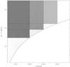 |
Fig. 2 Absolute magnitude of faint galaxies selected within the composite cylinder vs redshift. The lower envelope represents the apparent magnitude limit of the catalogue (r = 21). Grey boxes represent three volume limited samples defined as follows: −17 ≤ Mr − 5 log (h) ≤ −12.9 and z ≤ 0.02, −17 ≤ Mr − 5 log (h) ≤ −13.8 and z ≤ 0.03, −17 ≤ Mr − 5 log (h) ≤ −14.5 and z ≤ 0.04. |
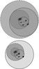 |
Fig. 3 Illustrations of two CGs and the projected cylinders around the centre of the minimum circle (where faint galaxies were selected), and around the 1st (or 2nd) ranked galaxies (where the density profiles are measured). Solid lines show the minimum circle and 3 times the minimum circle. Dashed lines show the circles centred in the 1st ranked galaxies and having radii of d12 and 2 d12. Galaxies shown in this figure represent only those considered as CG members (within a 3 mag range from the brightest). Upper plot: an extreme case where the centre of the profile is on the edge of the minimum circle that encloses the CG galaxy members and the separation between the two brightest galaxies is the diameter of the minimum circle. In this extreme case, the dashed line with radius d12 is the largest circle around the 1st or 2nd ranked galaxy that falls entirely within the cylinder defined for the search of faint galaxies (solid line). Lower plot: a generic case where the centre of the profile is also on the edge of the minimum circle that encloses the CG galaxy members, but now the separation between the two brightest galaxies is smaller than the radius of the minimum circle. In this case, it is possible to go farther than 2 d12 and still be complete in the sample of faint galaxies. |
4.2. Number density profiles: volume limited samples
Using a flux limited catalogue implies that groups at different redshifts are inhabited by different populations of galaxies in terms of their intrinsic luminosities.
Figure 2 shows the absolute magnitudes of galaxies selected within the group cylinders vs their redshifts. The lower envelope reproduces the apparent magnitude limit r = 21. To avoid possible biases related with incomplete sampling of galaxies in terms of luminosity, we defined three volume limited samples. The selected samples of faint galaxies lie in the grey boxes in Fig. 2, and are defined by the criteria:
-
−17 ≤ Mri − 5 log (h) ≤ −12.9 & zcm ≤ 0.02,
-
−17 ≤ Mri − 5 log (h) ≤ −13.8 & zcm ≤ 0.03,
-
−17 ≤ Mri − 5 log (h) ≤ −14.5 & zcm ≤ 0.04,
where Mri −5 log (h) is the galaxy absolute magnitude in the rSDSS band and zcm is the median redshift of the system.
Therefore, we computed the projected number density profiles of faint galaxies that belong to each of those complete subsamples around the first and second ranked galaxies of the groups, for CGs and control groups. To obtain statistically significant results, we built a composite group by stacking the groups normalised to a characteristic size. We adopted the projected distances between the first and second ranked galaxies, d12, as a normalisation size. After computing the number of faint galaxies within the areas of the projected rings around the first and second ranked galaxies, we divided the projected density by the number of groups that contributed to each bin of normalised distance.
It is worth mentioning here the influence of our choice of cylinders to look for the faint galaxies. In normal groups, we selected faint galaxies within 4 times the normalisation factor, d12, around the first ranked galaxy. Therefore, we can ensure that all groups contribute up to 4 times the d12 around the first ranked galaxy, and also we can ensure that all groups contribute at least up to 3 times the d12 around the second ranked galaxy. In both cases, we will only be interested in the profiles up to 3 times the normalisation distance.
In CGs, however, the cylinder in which the faint galaxies are selected was defined based on the CG criteria: centred in the centre of the minimum circle and spanning up to 3 times the size of that circle. However, given that the profiles will be centred in the first and second ranked galaxies, some considerations have to be taken into account. In the worst scenario shown in the upper plot of Fig. 3, the d12 may be as large as the diameter of the minimum circle (2 RG, where RG is the projected radius of the minimum circle). In such cases, the projected rings around the first ranked galaxy will be complete only up to a radius of d12, therefore for those groups we do not take into account the contribution of galaxies whose normalised distances to the first ranked galaxies are larger than 1. The same is valid when the second ranked galaxy is the centre of the profile. As the centre of the density profile (first or second ranked galaxy) is closer to the centre of the minimum circle or the separation between the first and second galaxies is shorter, the contribution of faint galaxies will span out to larger normalised distances, as is shown in the lower plot of Fig. 3. In addition, the number of groups that contribute in each bin of normalised distance varies accordingly.
Given that we are computing the projected number density profiles up to 3 times the normalisation size, and that we are carefully taking into account the proper normalisation of the group contributions, the different definitions of cylinders for compact and control groups do not affect the resulting projected number density profiles.
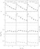 |
Fig. 4 Projected number density profiles of faint galaxies around the 1st ranked (black) and 2nd ranked galaxies (grey), split into three volume-limited samples (columns from left to right). Solid lines correspond to the profiles in CGs (CGS), while dotted lines are around the control group sample (S1). Error bars are the standard deviations computed with 100 bootstraps. Bottom panels: the ratios of the profiles around CGs and S1s. Errors are computed by error propagation. |
Figure 4 shows the projected number density profiles around the first (black) and second (grey) ranked galaxies, for CGs (solid lines) and control groups (dashed lines). Error bars are computed using 100 bootstrap resamplings. Each column corresponds to each of the different volume limited samples defined above. In the bottom panels of this figure, we show the ratio between the profiles of CGs and S1 around the first and second ranked galaxy. Error bars are computed by error propagation. We find that the number density of faint galaxies is larger around normal groups than around CGs. However, since the ratios are almost constant, the way these galaxies are distributed is very similar. In both CGs and S1 groups, faint galaxies mainly cluster around the brightest galaxy of the group which is reflected in a cuspier profile around the first ranked galaxy. As expected, the second brightest galaxy also gathers faint galaxies, but the effect is not as important as around the first ranked galaxy. In fact, the density of faint galaxies is determined by the brightness of the galaxies taken as centres rather than the ranking they have inside the group (see Appendix A).
At this point we analysed whether the differences in the sizes of the normalisation parameters in CGs and S1 could lead to the difference we found in the projected number density of faint galaxies. Therefore, we defined a subsample of CGs and a subsample of control groups in order to avoid any dependence of the profiles on the separation of the two brightest galaxies; we restricted both samples to those groups whose angular distance between the two brightest galaxies is 1.5 arcmin ≤ Θ12 ≤ 10 arcmin and matched the normalised Θ12 distributions. We refer to these subsamples as CGs2 and S2. The CGs2 sample comprises 78 CGs, while the S2 sample comprises 42 normal groups. Figure 5 shows the distribution of properties of CGs2 and S2 groups. From the comparison with Fig. 1, it can be seen that CGs with the brightest surface brightness have been excluded after restricting the separations between their two brightest galaxies, however, they have still brighter surface brightness than the control groups and have smaller projected radii.
We repeated the calculation of the projected number density profiles by splitting the faint galaxies into the three volume-limited samples defined above. The volume-limited subsamples comprise 30(12), 70(34), and 76(41) CGs2(S2), from the closest to the deeper volume, respectively. Figure 6 shows the profiles around these subsamples of groups that span the same range of normalising distances.
The projected number densities of faint galaxies in these new samples are different from those observed in Fig. 4. It can be seen that the profiles of faint galaxies are now very similar in CGs and control groups (CGs2 vs. S2). Taking into account the corresponding errors (which are large in the smallest volume limited sample given the low number of groups involved), we observe that the ratios among the projected number density profiles are almost constant and equal to unity in the three volume limited samples around the first ranked galaxy (black points/lines). The ratios around the second ranked galaxies also behave similarly to the former ratios, although CGs are underdense in the outskirts of the cylinders for the two deeper volume limited samples.
5. Comparison with observations
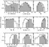 |
Fig. 5 Same as Fig. 1 for mock CGs2 (black empty histograms) and control groups S2 (grey histograms) after matching their angular distances between the 1st and 2nd ranked galaxies. Error bars correspond to Poisson errors. |
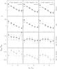 |
Fig. 6 Projected number density profiles of faint galaxies around the 1st ranked (black) and 2nd ranked galaxies (grey), split into three volume-limited samples (columns from left to right). Solid lines correspond to the profiles in CGs (CGs2), while dotted lines are around the control group sample (S2). Error bars are the standard deviations computed with 100 bootstraps. Bottom panels: ratios of the profiles around CGs2 and S2s. Errors are computed by error propagation. |
We used the sample of 2MCG identified in the 2MASS catalogue by Díaz-Giménez et al. (2012) and looked for faint neighbours in/around CGs from the spectroscopic data of the Sloan Digital Sky Survey data release 9 (SDSS DR9, Ahn et al. 2012) having apparent magnitudes brighter than rlim = 17.77. From the original 85 2MCGs, 45 of them lie in the SDSS area. For the purposes of this work, we have restricted the sample to CGs whose brightest galaxy is brighter than r = 13.27, and, we have checked that all the selected CGs fulfil the CG criteria in the r-band (they were originally identified as CGs in the Ks-band). These conditions reduced the sample to 30 CGs.
Because of the flux limit of this catalogue, faint neighbours were selected as being brighter than 17.77 (and excluding the members). Using the Catalog Archive Server Jobs System (CasJobs) of SDSS1, we found that 20 of the 30 CGs have 133 faint neighbours within 3ΘG, having | vi − ⟨ v ⟩ | < 1000 km s-1 and r< 17.77. The properties of these 20 groups are shown in Fig. 7 (grey histograms). We have checked that the properties of the 2MCGs that have or do not have neighbours in SDSS do not present differences. As previously reported in Díaz-Giménez et al. (2012), the 2MCG are typically biased towards lower memberships, fainter surface brightness, larger angular diameters, and separations between the two brightest galaxies compared to mock CGs (see Fig. 1).
To compare with the semi-analytical predictions, we used the sample of CGs2 defined in the previous section, and also restricted the sample to groups with radial velocity less than 10 000 km s-1 to match the observations. We applied the same conditions to the mock CGs as in the observations regarding the magnitude of the brightest galaxy and restricted the neighbours in the mock CGs within the same magnitude range. We found 72 CGs2 that satisfy that rbrightest ≤ 13.27, vr< 10 000 km s-1 and have 694 faint neighbours brighter than r = 17.77.
Given the low number of faint galaxies in the observational sample, introducing the absolute magnitude limit M ≥ −17 to define faint galaxies would reduce the number of objects, and would affect the statistical significance of the results. Therefore, we changed the criterion of magnitudes used to select faint neighbours, allowing the sample to contain all galaxies with apparent magnitudes brighter than 17.77, and excluding only the CG members (rbrightest ≤ r ≤ rbrightest + 3). However, working with flux limited catalogues implies that for different values of rbrightest, a different range of luminosities will be included in the search for faint galaxies. Then, around apparently bright galaxies (i.e. with bright apparent magnitudes), the range of faint galaxies included in the profiles will be larger than the corresponding range for galaxies that were not as bright in apparent magnitude, despite their intrinsic luminosity. Hence, we checked whether this change in the definition of faint neighbours introduces differences in the results previously found for volume limited samples for the semi-analytical galaxies. In Fig. 8, we show the number density profiles of faint galaxies selected in flux limited samples (rlim = 17.77) around simulated compact and control groups. The samples of compact and control groups are those defined as CGs2 and S2 in Sect. 4.2, having the same distribution of normalisation sizes. It can be seen that the ratios between the profiles around CGs control groups are consistent with the results obtained for volume-limited samples extracted from a deeper catalogue (rlim = 21, see Fig. 6) i.e., the distributions of faint galaxies around compact and normal groups are alike. This test allowed us to conclude that, provided the samples of faint neighbours around compact and control groups are selected under the same restrictions (flux- or volume-limited), the comparison between compact and control groups gives similar results. Thus, in order to compare observations with simulations, we applied this flux-limited criterion to select faint galaxies.
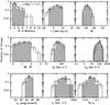 |
Fig. 7 Same as Fig. 1 for mock CGs2 (black empty histograms) and 2MASS CG with their faint galaxies extracted from the Sloan Digital Sky Survey (grey histograms). Error bars correspond to Poisson errors. In this figure, the mock CGs2 sample comprises the remaining groups after taking into account the observational incompleteness. |
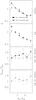 |
Fig. 8 Projected number density profiles of faint galaxies around the 1st ranked (black) and 2nd ranked (grey) galaxy of the groups. Upper panel: profiles for the mock CG (CGs2) sample while the second panel shows the profiles for the control groups (S2) shown in Fig. 5. Faint galaxies are selected having rbrightest + 3 <ri< 17.77. Error bars are the standard deviations computed with 100 bootstraps. Bottom panels: ratios between the profiles around CGs2 and the profiles around S2. Errors are computed by error propagation. |
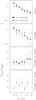 |
Fig. 9 Projected number density profiles of faint galaxies around the 1st ranked (black) and 2nd ranked galaxy of the groups (grey). Upper panel: profiles for the mock CG (CGs2) sample when incompleteness by fibre collision and low surface brightness are included; second panel: profiles for the CGs in the 2MASS (2MCGs) shown in Fig. 7. Faint galaxies in the 2MCGs are extracted from the SDSS. Error bars are the standard deviations computed with 100 bootstraps. Bottom panels: ratios between the profiles around CGs2 and the profiles around the 2MCGs. Dotted lines shows the corresponding ratios when no incompleteness is included in the mock sample. Errors are computed by error propagation. |
We included in our sample of mock CGs two well-known incompletenesses present in the SDSS, to allow a fair comparison between observations and simulations. We first considered the observational limitation of fibre collision in the spectroscopy of galaxies. Because of restrictions of fibre placement during the SDSS survey, two targets separated by less than 55′′ cannot be observed simultaneously on the same plate, but can both be observed on overlapping plates. This fibre collision effect reduces the number of pairs on small (one-halo) scales and therefore lowers the clustering strength over these small scales. Instead of correcting the observations by this effect, we have modified the mock catalogue by introducing the missing of close pairs of galaxies. We discarded one galaxy in each pair separated by less than 55′′: in the cases where the pair is formed by one galaxy selected as CG member, we discarded the neighbour; in the cases where the pair is formed by two non-members, we discarded one galaxy randomly. We chose to discard one galaxy in the 100% of those close galaxy pairs, which is a higher percentage than in observations, as an extreme case of incompleteness. Secondly, there is an incompleteness in the SDSS for very low surface brightness objects. The SDSS has a Petrosian half-light surface brightness (μ50) limit of 24.5 mag/arcsec2 and becomes incomplete for μ50> 23 mag/arcsec2. Even though this incompleteness is marginal in the range of magnitudes of galaxies involved in our work, we considered this effect in the semi-analytical faint galaxies. Since in the semi-analytical model the galaxies are point particles, we assigned surface brightness to each galaxy using the empirical prescriptions given by Shen et al. (2003) which relate the absolute magnitude in the rSDSS-band, Mr, with the half-light radius in physical units, R50, and the surface brightness with Mr and R50 (Eqs. (14), (15), and (20) in Shen et al. 2003). Using these estimates we discarded from the mock faint galaxy sample all galaxies with μ50> 23 mag/arcsec2. Therefore, our main mock faint galaxy sample is 100% incomplete owing to the missing pair problem and 100% incomplete for low surface brightness galaxies. Hence, under these restrictions, we found 69 CGs2 with 555 faint neighbours.
Figure 7 shows a comparison of the properties of the 69 CGs2 (black lines) and the 20 2MCGs that have faint neighbours around them in the spectroscopic SDSS sample (grey histograms). Both samples span similar ranges in the distribution of the group properties.
Regarding the projected number density profiles, we followed the same procedure as explained in Sect. 4.2. The number of galaxies that are effectively taken into account to compute the profiles are 83(58) around the first (second) ranked galaxies around 19(18) observable 2MCGs, and 393(337) faint galaxies around the first (second) ranked galaxies of 64(66) mock CGs. Figure 9 shows the profiles around the first and second ranked galaxies for mock CGs (solid lines) and the 2MCGs (dotted lines). Because of the low number of observational CGs (and faint galaxies around them), in this figure we show only those bins of normalised distance in which at least two observational galaxies contribute. This choice restricted the profiles within ~2 d12 from the central galaxies. From the ratios among the profiles shown in the two bottom panels (solid lines), it can be seen that, in spite of the large error bars resulting from the small number of galaxies involved, the distributions of the populations of faint galaxies around mock and observed CGs are statistically indistinguishable.
However, these results are a lower limit to the projected number density profiles given that we have overestimated the effect of the fibre collisions and the loss of low surface brightness galaxies. We also analysed the scenario where none of these effects are taken into account in the sample of faint semi-analytical galaxy neighbours. The results can be seen in the two bottom panels of Fig. 9 where dotted lines represent the ratios between the observed profiles and the simulated profiles without introducing any incompleteness. These results are an upper limit to the ratios between the simulated and observed projected number density profiles. Since the resulting ratios in the lower and upper limits are indistinguishable within the errors, we conclude that these observational incompleteness are not relevant for our comparison.
6. Summary
By definition, only galaxies within a three-magnitude range from the brightest galaxy of each group are considered as members of CGs. Isolation and compactness are defined based on the galaxy members, therefore fainter galaxies do not affect them. However, they do inhabit the same environment as the brighter galaxies in CGs and might feel the effect of an overdense environment in both, their abundance and their properties. In this work, we focused on the existence and distribution of faint galaxies in/around CGs.
To assess the question of whether the CG extreme environment affects the abundance of fainter galaxies, in this work we explored the projected number density profiles of the fainter population of galaxies in these systems. We compared our results with the profiles of the same population inhabiting normal groups.
Observationally, the study of the faint population of galaxies in CGs has been limited given the difficulties for detecting such galaxies. We faced the problem from a semi-analytical point of view by exploring the behaviour of the faint population of galaxies in the surroundings of groups extracted from mock catalogues built from synthetic galaxies extracted from a semi-analytical model of galaxy formation run on top of a numerical N-body dark matter simulation.
We chose the publicly available outputs of the Guo et al. (2011) semi-analytical model combined with the Millennium II simulations (Boylan-Kolchin et al. 2009) to construct a lightcone of galaxies with observable properties of galaxies. This model has been tuned to match the observable properties of galaxies at redshift zero, with particular emphasis on the faint galaxy population which makes it the most suitable with which to perform the analyses developed in this present work.
CGs were identified following the standard criteria established by Hickson (1982) modified to reproduce the largest and more complete sample of CGs that have been identified automatically from the 2MASS catalogue (Díaz-Giménez et al. 2012). Normal groups were identified using the standard FoF algorithm applied to a flux limited catalogue (Huchra & Geller 1982; Zandivarez et al. 2014).
We computed the projected number density profiles of faint galaxies in/around the main galaxies of groups and, in order to stack groups, we used as normalisation parameter the separation between the first and second ranked galaxies of the groups.
First, we observe that the shape of the projected number density profiles in the inner regions indicates that the faint galaxy population is more concentrated around the first ranked galaxy than around the second ranked galaxy, for CG and control samples. We found that CGs are underdense in faint galaxies when compared to normal groups; however, the shapes of the distribution of the faint populations around both types of systems are alike.
Given that one of the main differences between CGs and normal groups is the size of the normalisation parameter, we computed the profiles for subsamples of compact and normal groups with the same distribution of the normalisation sizes. This time, the projected number density profiles around the first ranked galaxies of compact and normal groups look alike, in shape and in height, indicating that there is no particular influence of the extreme CG environment on the number of faint galaxies in such groups.
We also compared the distribution of the faint population around semi-analytical and observational CGs. We used the observational CGs identified by Díaz-Giménez et al. (2012) that lie on the SDSS area, from where we extracted the fainter galaxies with spectroscopic information. Although the number of observational CGs and faint neighbours is small, this exercise allowed us to compare the predictions of the semi-analytical model to observations. We observed a similar behaviour of the population of faint galaxies in observations and simulations with the semi-analytical model of Guo et al. (2011). Different authors have performed similar comparisons but using different semi-analytical models and different types of groups. Weinmann et al. (2006) and Liu et al. (2010) found that previous versions of the semi-analytical models (Croton et al. 2006; Bower et al. 2006; Kang et al. 2005) overpredicted the satellite content of groups and clusters. However, Weinmann et al. (2011) found that the number density profile of faint galaxies (in a fixed absolute magnitude range) in massive clusters is accurately reproduced by the state-of-the-art semi-analytical models (Guo et al. 2011). In this work, we were able to extend this result to CGs. Nevertheless, we note the need for more observational data to perform a more reliable comparison.
Online material
Appendix A: Projected number density profiles for different classes of CGs: ranking vs. luminosity
We investigated what is the most important parameter in the determination of the centre around which the clustering of faint galaxies occurs in CGs, i.e. if faint galaxies are preferentially distributed around the most luminous galaxy (in which case the most important is the ranking of the galaxy) or around any luminous galaxy (most important parameter is the luminosity). Therefore, we studied the density profiles of faint galaxies around different subsamples of CGs classified according to different group properties. The criteria used to split the subsamples are:
-
Faint vs bright first ranked galaxy: we split the sample of CGs according to the absolute magnitude of the brightest galaxy of the system. Those having a brightest galaxy brighter than the 30th percentile of the distribution of absolute magnitudes of the first ranked galaxies of all the CGs are classified as
 , while CGs whose first ranked galaxy is fainter than the 70th percentile of the distribution of absolute magnitudes of the first ranked galaxies in the complete sample of CGs are
  .
. -
Dominated vs non-dominated groups: we split the sample of CGs according to the difference in absolute magnitude between the first and second ranked galaxies. CGs dominated by a very bright galaxy (Dom) will exhibit a larger difference between their two brightest members. We used the 30th and 70th percentiles of the distribution to split the sample into Dom and non-Dom CGs, respectively.
Faint galaxies are selected from a volume limited sample having −17 ≤ Mr − 5 log (h) ≤ −13.8 and zcm ≤ 0.03 (see Fig. 2). Figure A.1 shows the projected number density profiles of faint galaxies around different classes of CGs. It can be seen that
-
groups having the brighter first ranked galaxies are denser around the first and the second ranked galaxies (top panels);
-
the projected number density profiles around the first and second ranked galaxies of CGs non-dominated by a single galaxy are remarkably similar.
These two results lead us to conclude that faint galaxies are more frequent around bright galaxies, regardless of the ranking in the CG.
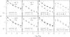 |
Fig. A.1 Projected number density profiles of faint galaxies around the 1st ranked (black) and 2nd ranked galaxy (grey) for different subsamples of CGs. Faint galaxies are defined within a volume limited sample with −17 ≤ Mr − 5log (h) ≤ −13.8 and zcm< 0.03. Top panels: CGs with bright/faint 1st ranked galaxies. Bottom panels: CGs dominated/non-dominated by a single bright galaxy. Error bars are the standard deviations computed with 100 bootstraps. |
Acknowledgments
We acknowledge the anonymous referee for insightful comments and suggestions that increased the general quality of the paper. The Millennium Simulation databases used in this paper and the web application providing online access to them were constructed as part of the activities of the German Astrophysical Virtual Observatory (GAVO). We thank Qi Guo for allowing public access for the outputs of her very impressive semi-analytical model of galaxy formation. Funding for SDSS-III has been provided by the Alfred P. Sloan Foundation, the Participating Institutions, the National Science Foundation, and the U.S. Department of Energy Office of Science. The SDSS-III web site is http://www.sdss3.org/. SDSS-III is managed by the Astrophysical Research Consortium for the Participating Institutions of the SDSS-III Collaboration including the University of Arizona, the Brazilian Participation Group, Brookhaven National Laboratory, Carnegie Mellon University, University of Florida, the French Participation Group, the German Participation Group, Harvard University, the Instituto de Astrofisica de Canarias, the Michigan State/Notre Dame/JINA Participation Group, Johns Hopkins University, Lawrence Berkeley National Laboratory, Max Planck Institute for Astrophysics, Max Planck Institute for Extraterrestrial Physics, New Mexico State University, New York University, Ohio State University, Pennsylvania State University, University of Portsmouth, Princeton University, the Spanish Participation Group, University of Tokyo, University of Utah, Vanderbilt University, University of Virginia, University of Washington, and Yale University. This work has been partially supported by Consejo Nacional de Investigaciones Científicas y Técnicas de la República Argentina (CONICET), Secretaría de Ciencia y Tecnología de la Universidad de Córdoba (SeCyT) and Fundação de Amparo à Pesquisa do Estado do São Paulo (FAPESP), through grants 2011/50471-4 and 2011/50002-4. CMdO acknowledges support of FAPESP (grant #2006/56213-9) and Conselho Nacional de Pesquisas (CNPq). H.G. thanks FAPESP for the IC grant #2012/04106-5.
References
- Ahn, C. P., Alexandroff, R., Allen de Prieto, C., et al. 2012, ApJS, 203, 21 [NASA ADS] [CrossRef] [Google Scholar]
- Amram, P., Mendes de Oliveira, C., Plana, H., & Balkowski, C. 2004, in Recycling Intergalactic and Interstellar Matter, eds. P.-A. Duc, J. Braine, & E. Brinks, IAU Symp., 217, 566 [Google Scholar]
- Berlind, A. A., Frieman, J., Weinberg, D. H., et al. 2006, ApJS, 167, 1 [NASA ADS] [CrossRef] [Google Scholar]
- Bower, R. G., Benson, A. J., Malbon, R., et al. 2006, MNRAS, 370, 645 [NASA ADS] [CrossRef] [Google Scholar]
- Boylan-Kolchin, M., Springel, V., White, S. D. M., Jenkins, A., & Lemson, G. 2009, MNRAS, 398, 1150 [NASA ADS] [CrossRef] [Google Scholar]
- Campos, P. E., Mendes de Oliveira, C., & Bolte, M. 2004, in Outskirts of Galaxy Clusters: Intense Life in the Suburbs, eds. A. Diaferio, IAU Colloq. 195, 441 [Google Scholar]
- Carrasco, E. R., Mendes de Oliveira, C., & Infante, L. 2006, AJ, 132, 1796 [NASA ADS] [CrossRef] [Google Scholar]
- Chilingarian, I. V., Melchior, A.-L., & Zolotukhin, I. Y. 2010, MNRAS, 405, 1409 [NASA ADS] [CrossRef] [Google Scholar]
- Croton, D. J., Springel, V., White, S. D. M., et al. 2006, MNRAS, 365, 11 [NASA ADS] [CrossRef] [Google Scholar]
- Da Rocha, C., Mieske, S., Georgiev, I. Y., et al. 2011, A&A, 525, A86 [NASA ADS] [CrossRef] [EDP Sciences] [Google Scholar]
- Díaz-Giménez, E. 2002, Master’s thesis, FaMAF, Universidad Nacional de Córdoba [Google Scholar]
- Díaz-Giménez, E., & Mamon, G. A. 2010, MNRAS, 409, 1227 [NASA ADS] [CrossRef] [Google Scholar]
- Díaz-Giménez, E., Mamon, G. A., Pacheco, M., Mendes de Oliveira, C., & Alonso, M. V. 2012, MNRAS, 426, 296 [NASA ADS] [CrossRef] [Google Scholar]
- Eke, V. R., Baugh, C. M., Cole, S., et al. 2004, MNRAS, 348, 866 [NASA ADS] [CrossRef] [Google Scholar]
- González, R. E., Lares, M., Lambas, D. G., & Valotto, C. 2006, A&A, 445, 51 [NASA ADS] [CrossRef] [EDP Sciences] [Google Scholar]
- Guo, Q., White, S., Boylan-Kolchin, M., et al. 2011, MNRAS, 413, 101 [NASA ADS] [CrossRef] [Google Scholar]
- Guo, Q., White, S., Angulo, R. E., et al. 2013, MNRAS, 428, 1351 [NASA ADS] [CrossRef] [Google Scholar]
- Henriques, B. M. B., White, S. D. M., Lemson, G., et al. 2012, MNRAS, 421, 2904 [NASA ADS] [CrossRef] [Google Scholar]
- Hernquist, L., Katz, N., & Weinberg, D. H. 1995, ApJ, 442, 57 [NASA ADS] [CrossRef] [Google Scholar]
- Hickson, P. 1982, ApJ, 255, 382 [NASA ADS] [CrossRef] [Google Scholar]
- Hickson, P., & Rood, H. J. 1988, ApJ, 331, L69 [NASA ADS] [CrossRef] [Google Scholar]
- Hickson, P., Ninkov, Z., Huchra, J. P., & Mamon, G. A. 1984, in Clusters and Groups of Galaxies, eds. F. Mardirossian, G. Giuricin, & M. Mezzetti, Astrophys. Space Sci. Lib., 111, 367 [Google Scholar]
- Huchra, J. P., & Geller, M. J. 1982, ApJ, 257, 423 [NASA ADS] [CrossRef] [Google Scholar]
- Kang, X., Jing, Y. P., Mo, H. J., & Börner, G. 2005, ApJ, 631, 21 [NASA ADS] [CrossRef] [Google Scholar]
- Kelm, B., & Focardi, P. 2004, A&A, 418, 937 [NASA ADS] [CrossRef] [EDP Sciences] [Google Scholar]
- Komatsu, E., Smith, K. M., Dunkley, J., et al. 2011, ApJS, 192, 18 [NASA ADS] [CrossRef] [Google Scholar]
- Konstantopoulos, I. S., Maybhate, A., Charlton, J. C., et al. 2013, ApJ, 770, 114 [NASA ADS] [CrossRef] [Google Scholar]
- Krusch, E., Rosenbaum, D., Dettmar, R.-J., et al. 2006, A&A, 459, 759 [NASA ADS] [CrossRef] [EDP Sciences] [Google Scholar]
- Liu, L., Yang, X., Mo, H. J., van den Bosch, F. C., & Springel, V. 2010, ApJ, 712, 734 [NASA ADS] [CrossRef] [Google Scholar]
- Mamon, G. A. 1986, ApJ, 307, 426 [NASA ADS] [CrossRef] [Google Scholar]
- McConnachie, A. W., Ellison, S. L., & Patton, D. R. 2008, MNRAS, 387, 1281 [NASA ADS] [CrossRef] [Google Scholar]
- Mendes de Oliveira, C., & Hickson, P. 1991, ApJ, 380, 30 [NASA ADS] [CrossRef] [Google Scholar]
- Prandoni, I., Iovino, A., & MacGillivray, H. T. 1994, AJ, 107, 1235 [NASA ADS] [CrossRef] [Google Scholar]
- Ribeiro, A. L. B., de Carvalho, R. R., & Zepf, S. E. 1994, MNRAS, 267, L13 [NASA ADS] [CrossRef] [Google Scholar]
- Rose, J. A. 1977, ApJ, 211, 311 [NASA ADS] [CrossRef] [Google Scholar]
- Shen, S., Mo, H. J., White, S. D. M., et al. 2003, MNRAS, 343, 978 [NASA ADS] [CrossRef] [Google Scholar]
- Spergel, D. N., Verde, L., Peiris, H. V., et al. 2003, ApJS, 148, 175 [NASA ADS] [CrossRef] [Google Scholar]
- Springel, V., White, S. D. M., Jenkins, A., et al. 2005, Nature, 435, 629 [NASA ADS] [CrossRef] [PubMed] [Google Scholar]
- Tovmassian, H. M., Yam, O., & Tiersch, H. 2001, Mex. Astron. Astrofis., 37, 173 [NASA ADS] [Google Scholar]
- Vulcani, B., De Lucia, G., Poggianti, B. M., et al. 2014, ApJ, 788, 57 [NASA ADS] [CrossRef] [Google Scholar]
- Walke, D. G., & Mamon, G. A. 1989, A&A, 225, 291 [NASA ADS] [Google Scholar]
- Wang, W., & White, S. D. M. 2012, MNRAS, 424, 2574 [NASA ADS] [CrossRef] [Google Scholar]
- Weinmann, S. M., van den Bosch, F. C., Yang, X., et al. 2006, MNRAS, 372, 1161 [NASA ADS] [CrossRef] [Google Scholar]
- Weinmann, S. M., Lisker, T., Guo, Q., Meyer, H. T., & Janz, J. 2011, MNRAS, 416, 1197 [NASA ADS] [CrossRef] [Google Scholar]
- Xu, G. 1995, ApJS, 98, 355 [NASA ADS] [CrossRef] [Google Scholar]
- Zabludoff, A. I., & Mulchaey, J. S. 1998, ApJ, 496, 39 [NASA ADS] [CrossRef] [Google Scholar]
- Zandivarez, A., Díaz-Giménez, E., Mendes de Oliveira, C., et al. 2014, A&A, 561, A71 [Google Scholar]
All Figures
|
Fig. 1 Distributions of observable properties of compact and control groups. Number of members in a three-magnitude range (top-left panel), radial velocity of the groups (top-centre panel), rest frame r-band absolute magnitude of the brightest galaxy member (top-right panel), difference in absolute magnitude between the brightest and the 2nd brightest galaxy of the groups (middle-left panel), projected radius of the minimum circle that encloses the galaxy members (middle-centre panel), projected distance between the brightest and 2nd brightest galaxies (middle-right panel), mean group surface brightness (bottom-left panel), radial velocity dispersion of the groups (bottom-centre panel), and dimensionless crossing time (bottom-right panel). Black empty histograms correspond to CGs (CGs), while grey histograms correspond to control groups (S1). Error bars correspond to Poisson errors. |
| In the text | |
|
Fig. 2 Absolute magnitude of faint galaxies selected within the composite cylinder vs redshift. The lower envelope represents the apparent magnitude limit of the catalogue (r = 21). Grey boxes represent three volume limited samples defined as follows: −17 ≤ Mr − 5 log (h) ≤ −12.9 and z ≤ 0.02, −17 ≤ Mr − 5 log (h) ≤ −13.8 and z ≤ 0.03, −17 ≤ Mr − 5 log (h) ≤ −14.5 and z ≤ 0.04. |
| In the text | |
|
Fig. 3 Illustrations of two CGs and the projected cylinders around the centre of the minimum circle (where faint galaxies were selected), and around the 1st (or 2nd) ranked galaxies (where the density profiles are measured). Solid lines show the minimum circle and 3 times the minimum circle. Dashed lines show the circles centred in the 1st ranked galaxies and having radii of d12 and 2 d12. Galaxies shown in this figure represent only those considered as CG members (within a 3 mag range from the brightest). Upper plot: an extreme case where the centre of the profile is on the edge of the minimum circle that encloses the CG galaxy members and the separation between the two brightest galaxies is the diameter of the minimum circle. In this extreme case, the dashed line with radius d12 is the largest circle around the 1st or 2nd ranked galaxy that falls entirely within the cylinder defined for the search of faint galaxies (solid line). Lower plot: a generic case where the centre of the profile is also on the edge of the minimum circle that encloses the CG galaxy members, but now the separation between the two brightest galaxies is smaller than the radius of the minimum circle. In this case, it is possible to go farther than 2 d12 and still be complete in the sample of faint galaxies. |
| In the text | |
|
Fig. 4 Projected number density profiles of faint galaxies around the 1st ranked (black) and 2nd ranked galaxies (grey), split into three volume-limited samples (columns from left to right). Solid lines correspond to the profiles in CGs (CGS), while dotted lines are around the control group sample (S1). Error bars are the standard deviations computed with 100 bootstraps. Bottom panels: the ratios of the profiles around CGs and S1s. Errors are computed by error propagation. |
| In the text | |
|
Fig. 5 Same as Fig. 1 for mock CGs2 (black empty histograms) and control groups S2 (grey histograms) after matching their angular distances between the 1st and 2nd ranked galaxies. Error bars correspond to Poisson errors. |
| In the text | |
|
Fig. 6 Projected number density profiles of faint galaxies around the 1st ranked (black) and 2nd ranked galaxies (grey), split into three volume-limited samples (columns from left to right). Solid lines correspond to the profiles in CGs (CGs2), while dotted lines are around the control group sample (S2). Error bars are the standard deviations computed with 100 bootstraps. Bottom panels: ratios of the profiles around CGs2 and S2s. Errors are computed by error propagation. |
| In the text | |
|
Fig. 7 Same as Fig. 1 for mock CGs2 (black empty histograms) and 2MASS CG with their faint galaxies extracted from the Sloan Digital Sky Survey (grey histograms). Error bars correspond to Poisson errors. In this figure, the mock CGs2 sample comprises the remaining groups after taking into account the observational incompleteness. |
| In the text | |
|
Fig. 8 Projected number density profiles of faint galaxies around the 1st ranked (black) and 2nd ranked (grey) galaxy of the groups. Upper panel: profiles for the mock CG (CGs2) sample while the second panel shows the profiles for the control groups (S2) shown in Fig. 5. Faint galaxies are selected having rbrightest + 3 <ri< 17.77. Error bars are the standard deviations computed with 100 bootstraps. Bottom panels: ratios between the profiles around CGs2 and the profiles around S2. Errors are computed by error propagation. |
| In the text | |
|
Fig. 9 Projected number density profiles of faint galaxies around the 1st ranked (black) and 2nd ranked galaxy of the groups (grey). Upper panel: profiles for the mock CG (CGs2) sample when incompleteness by fibre collision and low surface brightness are included; second panel: profiles for the CGs in the 2MASS (2MCGs) shown in Fig. 7. Faint galaxies in the 2MCGs are extracted from the SDSS. Error bars are the standard deviations computed with 100 bootstraps. Bottom panels: ratios between the profiles around CGs2 and the profiles around the 2MCGs. Dotted lines shows the corresponding ratios when no incompleteness is included in the mock sample. Errors are computed by error propagation. |
| In the text | |
|
Fig. A.1 Projected number density profiles of faint galaxies around the 1st ranked (black) and 2nd ranked galaxy (grey) for different subsamples of CGs. Faint galaxies are defined within a volume limited sample with −17 ≤ Mr − 5log (h) ≤ −13.8 and zcm< 0.03. Top panels: CGs with bright/faint 1st ranked galaxies. Bottom panels: CGs dominated/non-dominated by a single bright galaxy. Error bars are the standard deviations computed with 100 bootstraps. |
| In the text | |
Current usage metrics show cumulative count of Article Views (full-text article views including HTML views, PDF and ePub downloads, according to the available data) and Abstracts Views on Vision4Press platform.
Data correspond to usage on the plateform after 2015. The current usage metrics is available 48-96 hours after online publication and is updated daily on week days.
Initial download of the metrics may take a while.