| Issue |
A&A
Volume 572, December 2014
|
|
|---|---|---|
| Article Number | A2 | |
| Number of page(s) | 7 | |
| Section | Planets and planetary systems | |
| DOI | https://doi.org/10.1051/0004-6361/201424617 | |
| Published online | 18 November 2014 | |
Characterization of the planetary system Kepler-101 with HARPS-N⋆,⋆⋆
A hot super-Neptune with an Earth-sized low-mass companion
1 INAF − Osservatorio Astrofisico di Torino, via Osservatorio 20, 10025 Pino Torinese, Italy
e-mail: This email address is being protected from spambots. You need JavaScript enabled to view it.
2 Observatoire Astronomique de l’Université de Genève, 51 Ch. des Maillettes, 1290 Versoix, Switzerland
3 Dipartimento di Fisica e Astronomia “Galileo Galilei", Università di Padova, Vicolo dell’Osservatorio 3, 35122 Padova, Italy
4 INAF − Osservatorio Astronomico di Padova, Vicolo dell’Osservatorio 5, 35122 Padova, Italy
5 SUPA, Institute for Astronomy, Royal Observatory, University of Edinburgh, Blackford Hill, Edinburgh EH93 HJ, UK
6 Harvard-Smithsonian Center for Astrophysics, 60 Garden Street, Cambridge, Massachusetts 02138, USA
7 Centre for Star and Planet Formation, Natural History Museum of Denmark, University of Copenhagen, 1350 Copenhagen, Denmark
8 SUPA, School of Physics & Astronomy, University of St. Andrews, North Haugh, St. Andrews Fife, KY16 9SS, UK
9 INAF − Fundación Galileo Galilei, Rambla Jos Ana Fernandez Prez 7, 38712 Brea Baja, Spain
10 INAF − IASF Milano, via Bassini 15, 20133 Milano, Italy
11 INAF − Osservatorio Astronomico di Palermo, Piazza del Parlamento 1, 90124 Palermo, Italy
12 Centro de Astrofìsica, Universidade do Porto, Rua das Estrelas, 4150-762 Porto, Portugal
13 Department of Physics, University of Warwick, Gibbet Hill Road, Coventry CV4 7AL, UK
14 Cavendish Laboratory, J J Thomson Avenue, Cambridge CB3 0HE, UK
15 Astrophysics Research Centre, School of Mathematics and Physics, Queens University, Belfast, UK
Received: 16 July 2014
Accepted: 12 September 2014
Abstract
We characterize the planetary system Kepler-101 by performing a combined differential evolution Markov chain Monte Carlo analysis of Kepler data and forty radial velocities obtained with the HARPS-N spectrograph. This system was previously validated and is composed of a hot super-Neptune, Kepler-101b, and an Earth-sized planet, Kepler-101c. These two planets orbit the slightly evolved and metal-rich G-type star in 3.49 and 6.03 days, respectively. With mass Mp = 51.1-4.7+ 5.1 M⊕, radius Rp = 5.77-0.79+ 0.85 R⊕, and density ρp = 1.45-0.48+ 0.83 g cm-3, Kepler-101b is the first fully characterized super-Neptune, and its density suggests that heavy elements make up a significant fraction of its interior; more than 60% of its total mass. Kepler-101c has a radius of 1.25-0.17+ 0.19 R⊕, which implies the absence of any H/He envelope, but its mass could not be determined because of the relative faintness of the parent star for highly precise radial-velocity measurements (Kp = 13.8) and the limited number of radial velocities. The 1σ upper limit, Mp< 3.8 M⊕, excludes a pure iron composition with a probability of 68.3%. The architecture of the planetary system Kepler-101 − containing a close-in giant planet and an outer Earth-sized planet with a period ratio slightly larger than the 3:2 resonance − is certainly of interest for scenarios of planet formation and evolution. This system does not follow thepreviously reported trend that the larger planet has the longer period in the majority of Kepler systems of planet pairs with at least one Neptune-sized or larger planet.
Key words: planetary systems / stars: fundamental parameters / techniques: photometric / techniques: radial velocities / techniques: spectroscopic
Based on observations made with the Italian Telescopio Nazionale Galileo (TNG) operated on the island of La Palma by the Fundación Galileo Galilei of the INAF (Istituto Nazionale di Astrofisica) at the Spanish Observatorio del Roque de los Muchachos of the Instituto de Astrofisica de Canarias.
Table 2 is available in electronic form at http://www.aanda.org
© ESO, 2014
1. Introduction
Studies of planetary population synthesis within the context of the core accretion model (e.g., Ida & Lin 2008; Mordasini et al. 2009) suggest that the planetary initial mass function is characterized by physically significant minima and maxima. In particular, a minimum in the approximate range 30 ≲ Mp ≲ 70 M⊕ is understood as evidence for a dividing line between planets dominated in their interior composition by heavy elements, and giant gaseous planets that undergo runaway gas accretion. Recent theoretical work (Mordasini et al. 2012) has also reproduced the basic shape of the planetary mass − radius relation and its time evolution in terms of the fraction of heavy elements Z = MZ/M in a planet. In particular, the radius distribution is predicted to be bimodal, with a wide local minimum in the approximate range 6 ≲ Rp ≲ 8 R⊕ that roughly coincides with the minimum in the range of planetary masses indicated above. Furthermore, the possible architectures of multiple-planet systems have enjoyed considerable attention aimed at gauging the likelihood of the formation and survival of terrestrial-type planets interior and exterior to close-in higher-mass objects that have undergone Type I or II migration. In particular, recent investigations have not only shown that hot Earths might be found in systems in which disk material has been shepherded by a migrating giant (Raymond et al. 2008), or that water-rich terrestrial planets can still form in the habitable zones of systems containing a hot Jupiter (Fogg & Nelson 2007), but also that terrestrial planets could be found just outside the orbit of a hot Jupiter in configurations with a variable degree of dynamical interaction (Ogihara et al. 2013).
The class of transiting exoplanets is uniquely suited to provide powerful constraints on the theoretical predictions of the formation, structural, and dynamical evolution history of planetary systems such as those listed above. For example, the observed Rp − Mp diagram indicates a paucity of planets with properties intermediate between those of Neptune and Saturn. In particular, the mass bin between 30 and 60 M⊕ and the radius bin between 5 and 7 R⊕ are among the most underpopulated, although objects with these characteristics should be relatively easy to find in high-precision photometric and spectroscopic datasets. Furthermore, data from the Kepler mission indicate that for multiple-planet architectures in which one object is approximately Neptune-sized or larger, the larger planet is most often the planet with the longer period (Ciardi et al. 2013), and also that in general a lack of companion planets in hot-Jupiter systems is observed (e.g., Latham et al. 2011; Steffen et al. 2012).
In this work we combine Kepler photometry with high-precision radial-velocity measurements of the Kepler-101 two-planet system gathered in the context of the GTO program of the HARPS-N Consortium (Pepe et al. 2013; Dumusque et al. 2014). Kepler-101 was initially identified as Kepler object of interest 46 (KOI-46). It was subsequently validated by Rowe et al. (2014), who derived orbital periods of 3.49 d and 6.03 d, and planetary radii of 5.87 R⊕ and 1.33 R⊕ for Kepler-101b and Kepler-101c, respectively, and also carried out successful dynamical stability tests. Our combined spectroscopic and photometric analysis allows us to derive a dynamical mass for Kepler-101b and to place constraints on that of Kepler-101c. The much improved characterization of the Kepler-101 system permits us to identify the first fully characterized super-Neptune planet, and to provide the first observational constraints on the architecture of multiple-planet systems with close-in low-mass giants and outer Earth-sized objects in orbits close to resonance.
2. Data
2.1. Kepler photometry
Kepler-101 (see IDs, coordinates, and magnitudes in Table 1) is a relatively faint target (Kp = 13.8) for high-precision radial-velocity searches. It was observed by Kepler for almost four years, from quarter Q1 to quarter Q17, with the long-cadence (LC) temporal sampling of 29.4 min, and for ten months, from quarter Q4 to quarter Q7, in short-cadence (SC) mode, that is one point every 58.8 s. The medians of the errors of individual photometric measurements are 155 and 846 ppm for LC and SC data.
The Kepler light curve shows distinct transits of the 3.5 d transiting planet Kepler-101b, with a depth of ~0.1%. On the other hand, the transits of the Earth-sized companion Kepler-101c, with a period of 6.03 d and a depth of ~55 ppm, are embedded in the photon noise. They can be detected after removing the Kepler-101b transits and by using data from more than 4−5 quarters, because the phase-folded transit has a low signal-to-noise ratio (S/N) of ~11 when taking all the available LC measurements into account.
The simple-aperture-photometry1 (Jenkins et al. 2010) measurements were used for the characterization of Kepler-101b and c (Sect. 3) and were corrected for flux contamination by background stars that are located in the Kepler mask of our target. This amounts to only a few percent, as estimated by the Kepler team2.
No clear activity features with amplitude larger than ~400 ppm are seen in Kepler LC data, indicating that the host star is magnetically quiet.
2.2. Spectroscopic follow-up with HARPS-N
2.2.1. Radial-velocity observations
Forty spectra of Kepler-101, with exposure times of half an hour and an average S/N of 16 at 550 nm, were obtained with the high-resolution (R ~ 115 000) fiber-fed, optical echelle HARPS-N spectrograph, installed during Avril 2012 on the 3.57 m Telescopio Nazionale Galileo (TNG) at the Observatorio del Roque de los Muchachos, La Palma Island, Spain (Cosentino et al. 2012). HARPS-N is a near-twin of the HARPS instrument mounted at the ESO 3.6 m telescope in La Silla (Mayor et al. 2003) optimized for the measurement of high-precision radial velocities (≲1.2 m s-1 in 1 hr integration for a V ~ 12 mag, slowly rotating late-G/K-type dwarf). Spectroscopic measurements of Kepler-101 were gathered with HARPS-N in obj_AB observing mode, that is, without acquiring a simultaneous thorium-lamp spectrum. Indeed, for this faint target, the instrumental drift during one night is considerably lower than the photon noise uncertainties. The first ten spectra were taken between June and August 2012, before the readout of the red side of the charge-coupled device (CCD) failed, which occurred in late September 2012. Thirty additional measurements were collected from the end of May 2013 to the end of August 2013, after the replacement of the CCD.
HARPS-N spectra were reduced with the online standard pipeline, and radial velocities were measured by means of a weighted cross-correlation with a numerical spectral mask of a G2V star (Baranne 1996; Pepe et al. 2002). They are listed in Table 2 along with their 1σ photon-noise uncertainties3, which range from 5.5 to 12.5  , and bisector spans. HARPS-N radial velocities show a clear variation, with a semi-amplitude of 19.4 ± 1.8 m s-1, in phase with the Kepler-101b ephemeris as derived from Kepler photometry (see Fig. 1). As expected from the relative faintness of the host star for high-precision radial velocities and the limited number of HARPS-N measurements, the RV signal induced by the Earth-sized planet Kepler-101c is not detected, hence only an upper limit can be placed on its mass.
No correlation or anticorrelation between bisector spans and RVs is seen, as expected when RV variations are induced by planetary companions.
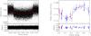 |
Fig. 1 Left panel: phase-folded short-cadence transit light curve of Kepler-101b along with the transit model (red solid line). Right panel: phase-folded radial-velocity curve of Kepler-101b and, superimposed, the Keplerian orbit model (black solid line). Red and blue circles show the HARPS-N data obtained with the original and replaced CCD. |
2.2.2. Stellar atmospheric parameters
We applied two slightly different approaches to derive the photospheric parameters of Kepler-101. The co-addition of all the available HARPS-N spectra (with resulting S/N = 96 at 550 nm) was analyzed using the same procedures as were described in detail by Sozzetti et al. (2004, 2006) and Dumusque et al. (2014), and references therein. A first set of relatively weak Fe I and Fe II lines was selected from the list of Sousa et al. (2010), and equivalent widths (EWs) were measured using the software TAME (Kang & Lee 2012). A second set of iron lines was chosen from the list of Biazzo et al. (2012), and EWs were measured manually. Effective temperature Teff, surface gravity log g, microturbulence velocity ξt, and iron abundance [Fe/H] were then derived under the assumption of local thermodynamic equilibrium (LTE), using the 2013 version of the spectral synthesis code MOOG (Sneden 1973), a grid of Kurucz ATLAS plane-parallel model stellar atmospheres (Kurucz 1993), and by imposing excitation and ionization equilibrium. Within the error bars, the two methods provided consistent results. The final adopted values, obtained as the weighted mean of the two independent determinations, are summarized in Table 1. They agree to within 1σ with the atmospheric parameters found independently with SPC (Buchhave et al. 2014). Both the low Vsini∗ = 2.6 ± 0.5 km s-1 and the average activity index  also indicate the low magnetic activity level of the host star inferred from the Kepler light curve.
3. Data analysis and system parameters
To determine the system parameters, a Bayesian combined analysis of HARPS-N and Kepler data was performed using a differential evolution Markov chain Monte Carlo (DE-MCMC) method (Ter Braak 2006; Eastman et al. 2013). SC Kepler data were used to model the transits of Kepler-101b, because they yield a more accurate solution than LC measurements by avoiding the distortion of the transit shape caused by the LC sampling (Kipping 2010). Specifically, eighty-two transits of Kepler-101b were observed in SC mode, which yields a S/N of ~190 for the phase-folded transit. On the other hand, LC measurements were used to perform the Kepler-101c transit modeling because SC data alone do not provide a high enough S/N. Indeed, fifty transits of Kepler-101c were observed with SC sampling, two-hundred and twenty-nine in LC mode. To perform the transit fitting, transits of Kepler-101b and c were individually normalized by fitting a linear function of time to the light-curve intervals of twice the transit duration before their ingress and after their egress.
System parameters of Kepler-101.
Since the RV signal of Kepler-101c is not detected in our HARPS-N data, we first performed a combined analysis of Kepler photometry and HARPS-N radial velocities of Kepler-101b by simultaneously fitting a transit model (Giménez 2006) and a Keplerian orbit. The free parameters of our global model are the transit epoch T0, the orbital period P, two systemic radial velocities for HARPS-N data obtained with both the original (Vr,o) and the replaced chip (Vr,r), the radial-velocity semi-amplitude K,  and
and  , where e is the eccentricity and ω the argument of periastron, the transit duration T14, the ratio of the planet to stellar radii Rp/R∗, the inclination i between the orbital plane and the plane of the sky, and the two limb-darkening coefficients (LDC) q1 = (ua + ub)2 and q2 = 0.5ua/ (ua + ub) (Kipping 2013), where ua and ub are the coefficients of the quadratic limb-darkening law (e.g., Claret 2000). A DE-MCMC analysis with a number of chains equal to twice the number of free parameters was then carried out. After removing the burn-in steps, as suggested by Knutson et al. (2009), and achieving convergence and a good mixing of the chains according to Ford (2006), the medians of the posterior distributions and their 34.13% intervals were evaluated and were taken as the final parameters and associated 1σ uncertainties. Mass, radius, and age of the host star were determined by comparing the Yonsei-Yale evolutionary tracks (Demarque et al. 2004) with the stellar effective temperature, metallicity, and density as derived from a/R⋆ and Kepler’s third law (see, e.g., Sozzetti et al. 2007; Torres et al. 2012). For this purpose, we considered normal distributions for the Teff and [Fe/H] with standard deviations equal to the uncertainties derived from our spectral analysis (Sect. 2.2.2). We used the same chi-square minimization as described in Santerne et al. (2011). Orbital, stellar, and Kepler-101b parameters are reported in Table 1. The SC photometric measurements and HARPS-N data phase-folded with the ephemeris of Kepler-101b are shown in Fig. 1 along with the best solution.
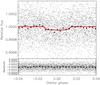 |
Fig. 2 Planetary transit of the Earth-sized planet Kepler-101c with the transit model (red solid line). Small circles show the phase-folded long-cadence Kepler data. Larger circles are the same data binned in 0.003 phase intervals for display purpose. |
The parent star Kepler-101 is a slightly evolved and metal-rich star, with a mass of  , a radius of 1.56 ± 0.20 R⊙, and an age of 5.9 ± 1.2 Gyr. According to orbital, transit, and the above-mentioned stellar parameters, Kepler-101b has mass, radius, and density of
  ,
,  , and
, and  . These values of mass and radius are in between those of Neptune and Saturn, earning Kepler-101b the name “super-Neptune”. Given its vicinity to the host star (a = 0.047 au), the equilibrium temperature is high: Teq ~ 1515 K. The inferred eccentricity of Kepler-101b is consistent with zero, although - given the current precision - a low eccentricity (<0.17 at 1σ) cannot be excluded.
The physical parameters of Kepler-101c were determined after those of Kepler-101b. The modeling of its transit was carried out by i) using all the available LC data; ii) considering a circular orbit4; iii) oversampling the transit model by a factor of 10 (e.g., Southworth 2012); and iv) fixing the LDC to the values that were previously derived because the low transit S/N prevents us from fitting them. The transit of Kepler-101c along with the best fit is shown in Fig. 2. A Bayesian DE-MCMC combined analysis of Kepler photometry and the residuals of HARPS-N data, after subtracting the Kepler-101b signal, indicates that this planet has a radius of  and a mass <3.78 M⊕. Indeed, as already mentioned, only an upper limit on the RV semi-amplitude of Kepler-101c can be given: K< 1.17 m s-1. Consequently, its bulk density is highly uncertain: ρp< 10.5 gcm-3. Finally, we point out that both the upper limit on the RV semi-amplitude of Kepler-101c and the orbital parameters of Kepler-101b were found to be fully consistent when modeling the RV data with two Keplerian orbits and imposing Gaussian priors on the orbital periods and transit epochs of Kepler-101b and c from Kepler photometry.
4. Discussion and conclusions
Thanks to forty precise spectroscopic observations obtained with HARPS-N and a Bayesian combined analysis of these measurements and Kepler photometry, we were able to characterize the planetary system Kepler-101. The system consists of a hot super-Neptune, Kepler-101b, at a distance of 0.047 au from the host star, and an outer Earth-sized planet, Kepler-101c, with a semi-major axis of 0.068 au and mass < 3.8 M⊕.
Figure 3 shows the positions of Kepler-101b and c in the radius-mass diagram of known exoplanets with radius Rp ≤ 12 R⊕, mass Mp< 500 M⊕, and precision on the mass better than 30%. Kepler-101b joins the rare known transiting planets in the transition region between Saturn-like and Neptune-like planets. A lower occurrence of giant planets in the mass interval 30 ≲ Mp ≲ 70 M⊕ is expected from certain models of planet formation through core accretion followed by planetary migration and disk dissipation (e.g., Mordasini et al. 2009; see their Fig. 3). This is most likely related to the fact that when a protoplanet reaches the critical mass to undergo runaway accretion (Pollack et al. 1996), its mass quickly increases up to 1−3 MJup. Therefore, disk dissipation might have occurred at the time of gas supply (Mordasini et al. 2009). Indeed, the X-ray and EUV energy flux from the parent star can account for a mass loss of <13 M⊕ during its lifetime of ~6 Gyr, according to Sanz-Forcada et al. (2011).
In terms of mass and radius, Kepler-101b is, to our knowledge, the first fully characterized super-Neptune. Indeed, seven known transiting planets with accurately measured masses have radii comparable with that of Kepler-101b at 1σ: CoRoT-8b, HAT-P-26b, Kepler-18c, Kepler-25b, Kepler-56b, Kepler-87c, and Kepler-89e. However, CoRoT-8b is a dense sub-Saturn with a higher mass than Kepler-101b, that is Mp = 69.9 ± 9.5 M⊕ (Bordé et al. 2010), and the remaining planets are low-density Neptunes with masses below ~25 M⊕. All the four planets with a mass similar to that of Kepler-101b, that is HAT-P-18b, Kepler-9b, Kepler-35b, and Kepler-89d, have larger radii of Rp> 8 R⊕.
According to models of the internal structure of irradiated (Fortney et al. 2007; Lopez & Fortney 2014) and nonirradiated (Mordasini et al. 2012) planets, the interior of Kepler-101b should contain a significant amount of heavy elements; more than 60% of its total mass. This might further support the observed correlation between the heavy element content of giant planets and the metallicity of their parent stars (Guillot 2008). Detailed modeling of the internal structure of the Earth-sized planet Kepler-101c is not possible because of the weak constraint on its mass of Mp< 3.8 M⊕ (<8.7 M⊕) at 1σ (2σ). We are only able to exclude a composition of pure iron with a probability of 68.3%, according to the models for solid planets by Seager et al. (2007) and Zeng & Sasselov (2013), and any H/He envelope from the planetary radius constraint (Rogers et al. 2011).
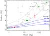 |
Fig. 3 Mass-radius diagram of the known transiting planets with radius Rp ≤ 12 R⊕, mass Mp< 500 M⊕, and precision on the mass better than 30%. Green diamonds indicate the Solar System giant planets Jupiter, Saturn, Neptune, Uranus, and the terrestrial planets Earth and Venus (from right to left). The three dotted lines indicate isodensity curves of 0.5, 1.5, and 5 g cm-3 (from top to bottom), and the blue solid lines show the mass and radius of planets consisting of pure water, 100% rocks, and 100% iron (Seager et al. 2007). The positions of Kepler-101b and c are plotted with red squares. |
We carried out a few N-body runs using a Hermite integrator (Makino 1991) to investigate the stability of the planetary system Kepler-101. The mass of the star and inner planet were set according to the values in Table 1, as were the semi-major axis and eccentricity of the inner planet. The semi-major axis of the outer planet was also set according to the value in Table 1, but we varied its mass and the initial eccentricity of its orbit. We ran each simulation for at least 108 orbits of the inner planet. Our simulations indicate that the system is stable for outer planet masses between one and four Earth masses and for outer planet eccentricities e ≤ 0.2. Orbit crossing would occur if the outer eccentricity exceeded e = 0.25, and none of our simulations with an outer planet eccentricity e ≥ 0.225 was stable. Hence, our results indicate that the system is stable for masses ≲4 M⊕ of the outer planet, in agreement with the 1σ upper limit from RV measurements, and for all eccentricities e ≲ 0.2.
Both planets in the Kepler-101 system are seen in transit, which means that these planets probably evolved through disk-planet interactions (Kley & Nelson 2012) and not through dynamical interactions (Rasio & Ford 1996). One proposed mechanism for forming close-in multiple planets is differential migration that forces the planets into a stable resonance, after which the planets migrate inward together (Lee & Peale 2002). That a large fraction of the known multiple planet systems are in mean motion resonance (MMR; Crida et al. 2008) would seem to be consistent with this picture. The Kepler-101 planets, however, are not in an MMR, and so this seems an unlikely formation scenario. On the other hand, the inner planet is close enough to the host star that it is likely that its orbit is influenced by a tidal interaction. Therefore, it is possible that the two planets did migrate inward in a 3:2 MMR but that the inner planet has since migrated farther inwards as a result of tidal effects (Delisle & Laskar 2014). Additionally, neither planet is massive enough to undergo gap-opening Type II migration (Lin & Papaloizou 1986), and so they would be expected to migrate in the faster Type I regime (Ward 1997). That the inner planet is more massive than the outer might also indicate that differential migration caused these planets to separate instead of migrating into a resonant configuration. Additionally, the density of Kepler-101b indicates that it might have formed beyond the snowline. Although we have no accurate density for Kepler-101c, the data would indicate that it has a composition consistent with formation inside the snowline. If this is true, it may be an example of a system in which an inner planet has survived the passage of a more massive outer planet, been scattered onto a wider orbit, and then migrated inward to its current position (Fogg & Nelson 2005; Cresswell & Nelson 2008). Indeed, the system Kepler-101 does not follow the trend observed for ~70% of Kepler planet pairs with at least one planet Neptune-sized or larger. In these systems, the larger planet typically has the longer period (Ciardi et al. 2013).
In conclusion, both the architecture of the planetary system Kepler-101 and the first full characterization of a super-Neptune are certainly of interest for a better understanding of planet formation and evolution, and for studying the internal structures of giant planets in the transition region between Neptune-like and Saturn-like planets.
Online material
HARPS-N radial velocities and bisector spans of Kepler-101.
RV jitter in our data is negligible as expected from the low magnetic activity level of Kepler-101.
A circular orbit was adopted for Kepler-101c in the absence of any RV constraint on orbital eccentricity. The latter, in any case, must be lower than 0.2 so as to avoid orbit crossing and system instability. See Sect. 4.
Acknowledgments
The HARPS-N project was funded by the Prodex Program of the Swiss Space Office (SSO), the Harvard University Origin of Life Initiative (HUOLI), the Scottish Universities Physics Alliance (SUPA), the University of Geneva, the Smithsonian Astrophysical Observatory (SAO), the Italian National Astrophysical Institute (INAF), University of St. Andrews, Queen’s University Belfast and University of Edinburgh. The research leading to these results has received funding from the European Union Seventh Framework Programme (FP7/2007-2013) under Grant Agreement No. 313014 (ETAEARTH). This research has made use of the results produced by the PI2S2 Project managed by the Consorzio COMETA, a co-funded project by the Italian Ministero dell’Istruzione, Università e Ricerca (MIUR) within the Piano Operativo Nazionale Ricerca Scientifica, Sviluppo Tecnologico, Alta Formazione (PON 20002006). X. Dumusque would like to thank the Swiss National Science Foundation (SNSF) for its support through an Early Postdoc Mobility fellowship. P. Figueira acknowledges support by Fundação para a Ciência e a Tecnologia (FCT) through the Investigador FCT contract of reference IF/01037/2013 and POPH/FSE (EC) by FEDER funding through the program “Programa Operacional de Factores de Competitividade − COMPETE”. R.D. Haywood acknowledges support from an STFC postgraduate research studentship. This publication was made possible through the support of a grant from the John Templeton Foundation. The opinions expressed in this publication are those of the authors and do not necessarily reflect the views of the John Templeton Foundation.
References
- Baranne, A., Queloz, D., Mayor, M., et al. 1994, A&AS, 119, 373 [Google Scholar]
- Biazzo, K., D’Orazi, V., Desidera, S., et al. 2012, MNRAS, 427, 2905 [NASA ADS] [CrossRef] [Google Scholar]
- Bordé, P., Bouchy, F., Deleuil, M., et al. 2010, A&A, 520, A66 [NASA ADS] [CrossRef] [EDP Sciences] [Google Scholar]
- Buchhave, L., Bizarro, M., Latham, D. W., et al. 2014, Nature, 509, 593 [NASA ADS] [CrossRef] [Google Scholar]
- Ciardi, D. R., Fabrycky, D. C., Ford, E. B., et al. 2013, ApJ, 763, 41 [NASA ADS] [CrossRef] [Google Scholar]
- Claret, A. 2000, A&A, 363, 1081 [NASA ADS] [Google Scholar]
- Cosentino, R., Lovis, C., Pepe, F., et al. 2012, in SPIE Conf. Ser., 8446 [Google Scholar]
- Cresswell, P., & Nelson, R. P. 2008, A&A, 482, 677 [NASA ADS] [CrossRef] [EDP Sciences] [Google Scholar]
- Crida, A., Sandor, Z., & Kley, W. 2008, A&A, 483, 325 [NASA ADS] [CrossRef] [EDP Sciences] [Google Scholar]
- Delisle, J.-B., & Laskar, J. 2014, A&A, 789, 154 [Google Scholar]
- Demarque, P., Woo, J.-H., Kim, Y.-C., & Yi, S. K. 2004, ApJS, 155, 667 [NASA ADS] [CrossRef] [Google Scholar]
- Dumusque, X., Bonomo, A. S., Haywood, R. D., et al. 2014, ApJ, 789, 154 [NASA ADS] [CrossRef] [Google Scholar]
- Eastman, J., Gaudi, B. S., & Agol, E. 2013, PASP, 125, 923 [Google Scholar]
- Fogg, M. J., & Nelson, R. P. 2005, A&A, 441, 791 [NASA ADS] [CrossRef] [EDP Sciences] [Google Scholar]
- Fogg, M. J., & Nelson, R. P. 2007, A&A, 461, 1195 [NASA ADS] [CrossRef] [EDP Sciences] [Google Scholar]
- Ford, E. B. 2006, ApJ, 642, 505 [NASA ADS] [CrossRef] [Google Scholar]
- Fortney, J. J., Marley, M. S., & Barnes, J. W. 2007, ApJ, 659, 1661 [NASA ADS] [CrossRef] [Google Scholar]
- Giménez, A. 2006, A&A, 450, 1231 [NASA ADS] [CrossRef] [EDP Sciences] [Google Scholar]
- Guillot, T. 2008, Phys. Scr., 130, id. 014023 [Google Scholar]
- Ida, S., & Lin, D. N. C. 2008, ApJ, 673, 487 [NASA ADS] [CrossRef] [Google Scholar]
- Jenkins, J. M., Caldwell, D. A., Chandrasekaran, H., et al. 2010, ApJ, 713, L87 [NASA ADS] [CrossRef] [Google Scholar]
- Kang, W., & Lee, S.-G. 2012, MNRAS, 425, 3162 [NASA ADS] [CrossRef] [Google Scholar]
- Kipping, D. 2010, MNRAS, 408, 1758 [NASA ADS] [CrossRef] [Google Scholar]
- Kipping, D. 2013, MNRAS, 435, 2152 [Google Scholar]
- Kley, W., & Nelson, R. P. 2012, ARA&A, 50, 211 [NASA ADS] [CrossRef] [Google Scholar]
- Knutson, H. A., Charbonneau, D., Cowan, N. B., et al. 2009, ApJ, 703, 769 [NASA ADS] [CrossRef] [Google Scholar]
- Kurucz, R. I. 1993, ATLAS9 Stellar Atmosphere Programs and 2 km s-1 grid. Kurucz CD-ROM No. 13 (Cambridge, Mass.: Smithsonian Astrophysical Observatory) [Google Scholar]
- Latham, D. W., Rowe, J. F., Samuel, N. Q., et al. 2011, ApJ, 732, L24 [NASA ADS] [CrossRef] [Google Scholar]
- Lee, M. H., & Peale, S. J. 2002, ApJ, 567, 596 [NASA ADS] [CrossRef] [Google Scholar]
- Lin, D. N. C., & Papaloizou, J. 1986, ApJ, 307, 395 [NASA ADS] [CrossRef] [Google Scholar]
- Lopez, E. D., & Fortney, J. J. 2014, ApJ, 792, 1 [NASA ADS] [CrossRef] [Google Scholar]
- Makino, J. 1991, ApJ, 369, 200 [NASA ADS] [CrossRef] [Google Scholar]
- Mayor, M., Pepe, F., Queloz, D., et al. 2003, The Messenger, 114, 20 [NASA ADS] [Google Scholar]
- Mordasini, C., Alibert, Y., Benz, W., & Naef, D. 2009, A&A, 501, 1161 [NASA ADS] [CrossRef] [EDP Sciences] [Google Scholar]
- Mordasini, C., Alibert, Y., Georgy, C., et al. 2012, A&A, 547, A112 [NASA ADS] [CrossRef] [EDP Sciences] [Google Scholar]
- Ogihara, M., Inutsukar, S.-I., Kobayashi, H., 2013, ApJ, 778, L9 [NASA ADS] [CrossRef] [Google Scholar]
- Pepe, F., Mayor, M., Galland, F., et al. 2002, A&A, 388, 632 [NASA ADS] [CrossRef] [EDP Sciences] [Google Scholar]
- Pepe, F., Cameron, A. C., Latham, D. W., et al. 2013, Nature, 503, 377 [NASA ADS] [CrossRef] [PubMed] [Google Scholar]
- Pollack, J. B., Hubickyj, O., Bodenheimer, P., et al. 1996, Icarus, 124, 62 [NASA ADS] [CrossRef] [Google Scholar]
- Rasio, F. A., & Ford, E. B. 1996, Science, 274, 954 [NASA ADS] [CrossRef] [PubMed] [Google Scholar]
- Rogers, L. A., Bodenheimer, P., Lissauer, J. J., & Seager, S. 2011, ApJ, 738, 59 [NASA ADS] [CrossRef] [Google Scholar]
- Rowe, J. F., Bryson, S. T., Marcy, G. W., et al. 2014, ApJ, 784, 45 [NASA ADS] [CrossRef] [Google Scholar]
- Raymond, S. N., Barnes, R., & Mandell, A. M. 2008, MNRAS, 384, 663 [NASA ADS] [CrossRef] [Google Scholar]
- Santerne, A., Díaz, R. F., Bouchy, F., et al. 2011, A&A, 528, A63 [NASA ADS] [CrossRef] [EDP Sciences] [Google Scholar]
- Sanz-Forcada, J., Micela, G., Ribas, I., et al. 2011, A&A, 531, A6 [NASA ADS] [CrossRef] [EDP Sciences] [Google Scholar]
- Seager, S., Kuchner, M., Hier-Majumder, C. A., & Militzer, B., et al. 2007, ApJ, 669, 1279 [NASA ADS] [CrossRef] [Google Scholar]
- Sneden, C. A. 1973, Ph.D. Thesis, The University of Texas at Austin [Google Scholar]
- Sozzetti, A., Yong, D., Torres, G., et al. 2004, ApJ, 616, L167 [NASA ADS] [CrossRef] [Google Scholar]
- Sozzetti, A., Yong, D., Carney, B. W., et al. 2006, AJ, 131, 2274 [NASA ADS] [CrossRef] [Google Scholar]
- Sozzetti, A., Torres, G., Charbonneau, D., et al. 2007, ApJ, 664, 1190 [NASA ADS] [CrossRef] [Google Scholar]
- Sousa, S. G., Alapini, A., Israelian, G., & Santos, N. C. 2010, A&A, 512, A13 [NASA ADS] [CrossRef] [EDP Sciences] [Google Scholar]
- Southworth, J. 2012, MNRAS, 426, 1292 [Google Scholar]
- Steffen, J. H., Fabrycky, D. C., Ford, E. B., et al. 2012, MNRAS, 421, 2342 [NASA ADS] [CrossRef] [Google Scholar]
- Ter Braak, C. J. F. 2006, Statistics and Computing, 16, 239 [Google Scholar]
- Torres, G., Fischer, D. A., Sozzetti, A., et al. 2012, ApJ, 757, 161 [NASA ADS] [CrossRef] [Google Scholar]
- Ward, W. R. 1997, Icarus, 126, 261 [NASA ADS] [CrossRef] [Google Scholar]
- Zeng, L., & Sasselov, D. 2013, PASP, 125, 227 [NASA ADS] [CrossRef] [Google Scholar]
All Tables
All Figures
|
Fig. 1 Left panel: phase-folded short-cadence transit light curve of Kepler-101b along with the transit model (red solid line). Right panel: phase-folded radial-velocity curve of Kepler-101b and, superimposed, the Keplerian orbit model (black solid line). Red and blue circles show the HARPS-N data obtained with the original and replaced CCD. |
| In the text | |
|
Fig. 2 Planetary transit of the Earth-sized planet Kepler-101c with the transit model (red solid line). Small circles show the phase-folded long-cadence Kepler data. Larger circles are the same data binned in 0.003 phase intervals for display purpose. |
| In the text | |
|
Fig. 3 Mass-radius diagram of the known transiting planets with radius Rp ≤ 12 R⊕, mass Mp< 500 M⊕, and precision on the mass better than 30%. Green diamonds indicate the Solar System giant planets Jupiter, Saturn, Neptune, Uranus, and the terrestrial planets Earth and Venus (from right to left). The three dotted lines indicate isodensity curves of 0.5, 1.5, and 5 g cm-3 (from top to bottom), and the blue solid lines show the mass and radius of planets consisting of pure water, 100% rocks, and 100% iron (Seager et al. 2007). The positions of Kepler-101b and c are plotted with red squares. |
| In the text | |
Current usage metrics show cumulative count of Article Views (full-text article views including HTML views, PDF and ePub downloads, according to the available data) and Abstracts Views on Vision4Press platform.
Data correspond to usage on the plateform after 2015. The current usage metrics is available 48-96 hours after online publication and is updated daily on week days.
Initial download of the metrics may take a while.