| Issue |
A&A
Volume 571, November 2014
|
|
|---|---|---|
| Article Number | A50 | |
| Number of page(s) | 16 | |
| Section | Planets and planetary systems | |
| DOI | https://doi.org/10.1051/0004-6361/201424211 | |
| Published online | 06 November 2014 | |
Deformation and tidal evolution of close-in planets and satellites using a Maxwell viscoelastic rheology
1
Departamento de Física, I3N, Universidade de Aveiro,
Campus de Santiago,
3810-193
Aveiro,
Portugal
e-mail:
This email address is being protected from spambots. You need JavaScript enabled to view it.
2
ASD, IMCCE-CNRS UMR8028, Observatoire de Paris, UPMC,
77 Av. Denfert-Rochereau,
75014
Paris,
France
3
Instituto de Geociências e Ciências Exatas, UNESP,
Av. 24-A 1515,
CEP 13506-900, Rio Claro, SP, Brazil
Received: 14 May 2014
Accepted: 24 September 2014
Abstract
In this paper we present a new approach to tidal theory. Assuming a Maxwell viscoelastic rheology, we compute the instantaneous deformation of celestial bodies using a differential equation for the gravity field coefficients. This method allows large eccentricities and it is not limited to quasi-periodic perturbations. It can take into account an extended class of perturbations, including chaotic motions and transient events. We apply our model to some already detected eccentric hot Jupiters and super-Earths in planar configurations. We show that when the relaxation time of the deformation is larger than the orbital period, spin-orbit equilibria arise naturally at half-integers of the mean motion, even for gaseous planets. In the case of super-Earths, these equilibria can be maintained for very low values of eccentricity. Our method can also be used to study planets with complex internal structures and other rheologies.
Key words: celestial mechanics / planets and satellites: general
© ESO, 2014
1. Introduction
The occurrence, on most open ocean coasts, of high sea tide at about the time of the Moon’s passage across the meridian, gave ancient observers the idea that our satellite exerts an attraction on the water, although the occurrence of a second high tide when the Moon is on the opposite meridian was a great puzzle. The correct explanation for tides was first indicated by Newton (1760) in the Philosophiæ Naturalis Principia Mathematica. They result from a differential effect of the gravitational force acting in accordance with laws of mechanics, since this force is not constant across the diameter of the Earth. Kant (1754) suggested that the Moon not only pulls the Earth, but also exerts a retarding torque upon its surface, this torque slowing down the Earth’s rotation until terrestrial days become as long as lunar months.
The estimates for the tidal deformation of a body are based on a very general formulation of the tidal potential, initiated by Darwin (1879). Assuming a homogeneous Earth consisting of an incompressible fluid with constant viscosity, Darwin derived a tide-generated disturbing potential expanded into a Fourier series. Thus, he was able to obtain the tidal contribution to the spin and orbital evolution, confirming Kant’s prediction (Darwin 1880). Ever since, many authors improved Darwin’s work, leading to a better understanding of this problem (e.g., Kaula 1964; MacDonald 1964; Alexander 1973; Singer 1968; Mignard 1979; Efroimsky & Williams 2009; Ferraz-Mello 2013).
All previous studies have shown the existence of a stationary solution for the rotation rate, which is synchronous when the two bodies move in circular orbits, but becomes super-synchronous for elliptical orbits. Standard tidal models consider an elastic tide and delay the tidal bulge by an ad hoc phase lag in order to take into account the body anelasticity (e.g., Kaula 1964; MacDonald 1964). However, these models are unable to explain the dependency of phase lag with the tidal frequency, which is a crucial point when we aim to study the long-term secular evolution of the planets.
If one adopts a linear model where the phase lag is proportional to the tidal frequency, i.e, a viscous model, the ratio between the orbital and rotational periods have an excess proportional to the square of the eccentricity, an equilibrium often called pseudo-synchronous rotation (e.g., Mignard 1979). However, this prediction is not confirmed by observations of the rotation of most planetary satellites (which are synchronous in non-eccentric orbits) or of the planet Mercury. One way to obtain a synchronous stationary solution is to assume that an additional torque, due to a permanent equatorial asymmetry (a quadrupolar approximation for the body’s figure), is acting on the body to counterbalance the tidal torque (Colombo 1965; Goldreich & Peale 1966). The stationary solutions obtained from the combination of both torques are called spin-orbit resonances, for which the synchronous motion is a particular case.
A more realistic approach to deal with the dependency of the phase lag with the tidal frequency is to assume a viscoelastic rheological model. One of the simplest models of this kind is to consider that the planet behaves like a Maxwell material, i.e., the material is represented by a purely viscous damper and a purely elastic spring connected in series (e.g., Turcotte & Schubert 2002). In this case, the planet can respond as an elastic solid or as a viscous fluid, depending on the frequency of the perturbation. Viscoelastic rheologies have been used recently (e.g., Henning et al. 2009; Remus et al. 2012a), since they are able to reproduce the main features of tidal dissipation, including the pseudo-synchronous rotation or the spin-orbit equilibria (e.g. Storch & Lai 2014). For a review of the main viscoelastic models see Henning et al. (2009).
Efroimsky (2012) describes the rheology of a planet using an empirical power scaling law for the phase lag which is consistent with the accumulated geophysical, seismological, and geodetic observational data. It is shown that the best fitted laws are in conformity with Andrade’s model (Andrade 1910), where the phase lag is inversely proportional to the tidal frequency. The Andrade model can be thought of as the Maxwell model equipped with an extra term describing hereditary reaction of strain to stress (Efroimsky 2012). However, Andrade’s model is extremely complex and the main features of tidal evolution are similar to other viscoelastic models.
Ferraz-Mello (2013) abandons the potential description introduced by Darwin, and proposes to study tides directly from the deformation law of the planet. For that purpose, he adopts a simple Newtonian creep model for the surface deformation, where the distance to the equilibrium is considered as proportional to the stress. As a result, the planet’s surface tends to the equilibrium spheroid, but not instantaneously. The resulting stationary rotations have an average excess velocity which depends on a critical frequency, the relaxation factor, which is inversely proportional to the viscosity of the body. Moreover, the dissipation in the pseudo-synchronous solution presents two regimes of variation, depending on the tidal frequency: in the inviscid limit, it is roughly proportional to the frequency (as in standard theories), but that behavior is inverted when the viscosity is high and the tidal frequency larger than the critical frequency, as in the model proposed by Efroimsky (2012).
An important setback in Ferraz-Mello (2013) model is the absence of an elastic tide. Indeed, when the tidal frequency is larger than the critical frequency, the phase lag tends to 90°, which is in contradiction with the observations done for most rocky planets. In order to conciliate the theory and the observed tidal bulges, we have to assume that the tide is not restricted to the component due to the creeping of the body under the tidal action, but has also a pure elastic component. This supposition was already present in Darwin’s original work (Darwin 1879), who realized that viscoelastic deformations of the planet’s surface could be derived from the Newtonian creep law.
In this paper we pursue in the same direction of Ferraz-Mello (2013), but we adopt a deformation law for the planet that is compatible with the viscoeslatic rheology of a Maxwell body (Sect. 2). We then compute the general solution for the deformation of the planet (Sect. 3), and use it to obtain the tidal evolution of the planet (Sect. 4). We also identify the equilibrium positions for the tidal torque (Sect. 5), and inspect the effect from some libration of the rotation rate around these equilibria (Sect. 6). We finally perform numerical simulations for some known close-in exoplanets (Sect. 7) and discuss the results in the last section.
2. Model
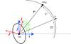 |
Fig. 1 Reference angles and notations. (i,j,k) is a fixed inertial reference frame, while (I,J,K) is a reference frame fixed in the planet. k = K are orthogonal to the orbit, and thus not shown. r is the radius vector from m to m0, P is the direction of pericenter, ϖ is the longitude of pericenter, and v is the true anomaly. The rotation angle θ is referred to the fixed reference direction i. We also use the angles |

We consider a system consisting of a central star of mass m0, and a companion planet of mass m. The planet is considered an oblate ellipsoid with gravity field coefficients given by J2, C22 and S22, sustained by the reference frame (I,J,K), where K is the axis of maximal inertia (Fig. 1). We furthermore assume that the spin axis of the planet, with rotation rate Ω, is also along K (gyroscopic approximation), and that K is orthogonal to the orbital plane (which corresponds to zero obliquity). The gravitational potential of the planet at the star is then given by (e.g., Correia & Rodríguez 2013)  (1)where
  (2)G is the gravitational constant, R is the mean planet radius, r is the position of the star with respect to center of mass of the planet, and
  is the unit vector. We neglect terms in (R/r)3 (quadrupolar approximation).
2.1. Deformation of the planet
The mass distribution inside the planet, characterized by the gravity field coefficients, is a result of the forces acting on it, that is, self gravity and the planet’s response to any perturbing potential, Vp. Here, we consider that the planet deforms under the action of the centrifugal and tidal potentials. Thus, on the planet’s surface, R, the non-spherical contribution of the perturbing potential is given by (e.g., Correia & Rodríguez 2013)  (3)We let ζ(R) be the radial deformation of the free surface. In the case of a homogeneous incompressible elastic solid sphere, the equilibrium surface deformation ζe(R) is given by (Kelvin 1863a,b; Love 1911)
  (4)where g = Gm/R2 is the surface gravity, and
  (5)is the second Love number associated with the radial displacement, ρ the density, and μ the rigidity (or shear modulus). Darwin (1879) extended the results to a homogeneous incompressible viscous body and obtained the differential equation
  (6)where hf = 5/2 is the fluid Love number1,
  (7)is the fluid relaxation time, and η is the viscosity. Darwin (1879) also realized that viscoelastic deformations can easily be derived from expression (6) using the substitution
  (8)where τe = η/μ is the elastic or Maxwell relaxation time. As a result, we obtain (Darwin 1879)
  (9)Finally, the deformation ζ of the body generates an additional potential V′(r) given by
  (10)In the case of quadrupolar deformations, as considered here (Eq. (1)), the additional potential exterior to the body (r ≥ R) is
  (11)Thus, at the mean radius (r = R), the additional potential must satisfy
 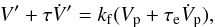 (12)where kf = 3/2 is the fluid second Love number for potential1. The equilibrium potential Ve is obtained for static perturbations or instantaneous response (τ = τe = 0)
 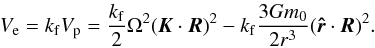 (13)The instantaneous variation of the additional potential V′ that results from the perturbation Vp, can then be obtained from the equilibrium potential Ve through expression (12) as
 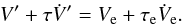 (14)We note that this viscoelastic deformation law is also fully compatible with a viscous rheology (Eq. (6)), provided that we set τe = 0. Previous expression could also have been obtained in the Fourier domain (see Appendix A).
2.2. Equations of motion
The force between the star and the planet is easily obtained from the gravitational potential of the system (Eq. (1)) as F = −m0 × ∇V(r). From this force we can directly obtain the orbital evolution of the system  , and the spin evolution
  (using the conservation of the total angular momentum of the system), where β = m0m/ (m0 + m) is the reduced mass of the system, and C is the principal inertia moment of the planet. Expressing
  and I = (cosθ, sin θ), where f is the true longitude and θ is the rotation angle, we thus have
 ![Mathematical equation: \begin{eqnarray} \ddvr = & - & \frac{\mug}{r^2} \ur - \frac{3 \mug R^2}{2 r^4} J_2 \, \ur - \frac{9 \mug R^2}{r^4} \left[ C_{22} \cos \dgam - S_{22} \sin \dgam \! \phantom{\frac{}{}} \right] \ur \crm & + & \frac{6 \mug R^2}{r^4} \left[ C_{22} \sin \dgam + S_{22} \cos \dgam \! \phantom{\frac{}{}} \right] \vk \times \ur , \label{130104b} \end{eqnarray}](/articles/aa/full_html/2014/11/aa24211-14/aa24211-14-eq66.png) (15)and
(15)and ![Mathematical equation: \begin{eqnarray} \ddot \theta \!&=&\! - \frac{6 G \M \m R^2}{C r^3} \left[ C_{22} \sin \dgam + S_{22} \cos \dgam \! \phantom{\frac{}{}} \right] , \label{130104d} \end{eqnarray}](/articles/aa/full_html/2014/11/aa24211-14/aa24211-14-eq67.png) (16)where μ0 = G(m0 + m), and γ = θ − f (Fig. 1).
(16)where μ0 = G(m0 + m), and γ = θ − f (Fig. 1).
Because the planet is not rigid and can be deformed under the action of a perturbing potential, the gravity field coefficients J2, C22 and S22 are not constant. Indeed, according to the deformation law given by expression (14) we have
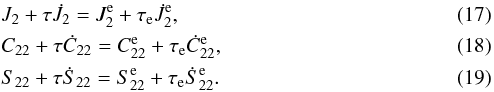 The equilibrium values for each coefficient are easily obtained comparing expressions (1) and (13), which gives (Correia & Rodríguez 2013)
 ![Mathematical equation: \begin{eqnarray} \label{130104e} &&J_2^\eq = \kf \left[ \frac{\om^2 R^3}{3 G \m} + \frac{1}{2} \frac{\M}{\m} \left(\frac{R}{r} \right)^3 \right], \\ \label{130104f} &&C_{22}^\eq = \frac{\kf}{4} \frac{\M}{\m} \left(\frac{R}{r}\right)^3 \cos \dgam , \\ \label{130104g}&&S_{22}^\eq = - \frac{\kf}{4} \frac{\M}{\m} \left(\frac{R}{r}\right)^3, \end{eqnarray}](/articles/aa/full_html/2014/11/aa24211-14/aa24211-14-eq71.png) and for their time derivatives, respectively
and for their time derivatives, respectively ![Mathematical equation: \begin{eqnarray} \label{130107e}&&\dot J_2^{\eq} = \kf \left[ \frac{2 \om R^3}{3 G \m} \dot\om - \frac{3}{2} \frac{\M}{\m} \left(\frac{R}{r}\right)^3 \frac{\dvr \cdot \vr}{r^2} \right] , \\ \label{130107f}&&\dot C_{22}^{\eq} = - \frac{\kf}{4} \frac{\M}{\m} \left(\frac{R}{r}\right)^3 \left[ 3 \frac{\dot r}{r} \cos \dgam + 2 \dot \gam \sin \dgam \right] , \\ \label{130107g}&&\dot S_{22}^{\eq} = \frac{\kf}{4} \frac{\M}{\m} \left(\frac{R}{r}\right)^3 \left[ 3 \frac{\dot r}{r} \sin \dgam - 2 \dot \gam \cos \dgam \right] . \end{eqnarray}](/articles/aa/full_html/2014/11/aa24211-14/aa24211-14-eq72.png) It should be noted that for the equilibrium solution (Eqs. (21), (22)), we have
It should be noted that for the equilibrium solution (Eqs. (21), (22)), we have  (Eq. (16)).
3. General solution
Introducing the complex notations  (26)we can rewrite Eqs. (18) and (19) together as
  (27)
(27)
The solution of Eq. (27) without the second hand member is Z = Z0e−t/τ, and the variation of the constant Z0 gives the general solution of Eq. (27)  (28)where
  is an integration constant. Although one can search for a solution of this equation in the precise setting of this paper, it is much more efficient to solve it first in a very general setting where Ze is a general almost periodic function, that is an expression of the form
  (29)where βk are constants, and ωk are a numerable set of fixed frequencies. The result is
  (30)The first term is the stationnary mode and the second one the transient mode that will decay rapidly to zero with time. In general, the constant in Eq. (30) is different from that of Eq. (28). It should be noted that here we do not have small divisors problems as the denominators 1 + iτωk never vanish. A constant term βk0 in Ze (corresponding to ωk0 = 0) will add an equivalent constant contribution βk0 to Z.
4. Tidal evolution
From the general solution of Eq. (27), we can study more specific solutions. For this, we will look to the explicit expression of Ze. Using expressions (21) and (22), we can write 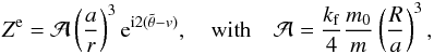 (31)where a is the semi-major axis,
  , ϖ is the longitude of the pericenter, and v is the true anomaly (Fig. 1). Using the expansion of (a/r)3exp(−2iv) in terms of Hansen coefficients
  (e.g., Hughes 1981) (see also Appendix C),
 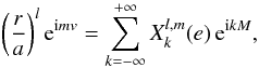 (32)we obtain
 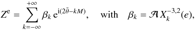 (33)where M is the mean anomaly, and e is the eccentricity. βk depends only on the orbital parameters that are assumed to be constant over one revolution. The evolution of θ is given by Eq. (16), but since tidal effects are usually very weak, in a zero order solution, we can also neglect
  , and assume that the rotation rate
  is constant over one orbital revolution. Thus, we can write
  (34)where n = Ṁ, and ωk is a constant frequency. As the βk are constant in Eq. (29), we are in a special case of the application of the results of Sect. 3, and we obtain, after neglecting the transtient part of expression (30) that decays to zero for t ≫ τ,
  (35)
(35)
 |
Fig. 2 Evolution of the second Love number k2, the dissipation Q-factor, and phase lag k2sinδ as a function of the tidal frequency ω (normalized by the relaxation time τ). For all parameters there is a transition of regime around τω ~ 1. We use here the Earth values for the Love numbers, ke = 0.3 and kf = 0.9 (Yoder 1995). |
4.1. Tidal torque
We have already seen that for Z = Ze,  , as there are no coupling torques in the problem due to alignment of the planet deformation with the star. It is then useful to use the difference
  (36)Denoting
  (37)we obtain the variations of
  in the first order solution
 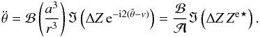 (38)where ℑ(z) denotes the imaginary part of z and z⋆ its complex conjugate. We thus see from expression (36) that θ disappears from the expression of . After an expansion in Hansen coefficients of expression (38), we obtain an explicit expression of with respect to the mean anomaly M
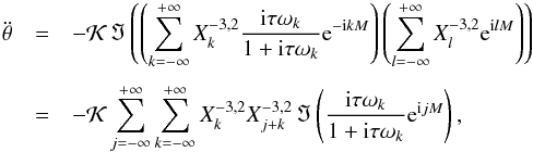 (39)where
 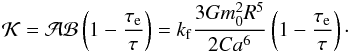 (40)The first order secular evolution of over one orbital period is easily obtained by averaging expression (39) over M, which is equivalent to keep only the terms with j = 0. We thus get
  , with the secular torque T given by
 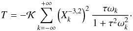 (41)
(41)
4.2. Relation with classical notations
Expressions (35) and (41) can be related to classical tidal parameters, by transforming the complex notation in a real amplitude and a phase lag  (42)and
  (43)with
  (44)and
  (45)We then conclude that the C22 and S22 are shifted by an angle δk with respect to the perturbation, and weakened by a factor of k2(ωk) /kf (Fig. 2). The phase lag δk (Eq. (44)) is zero for ωk = 0 and ωk → ∞, and its maximal value is obtained at the frequency ωk = (ττe)−1/2. The amplitude k2(ωk) is monotonically decreasing with ωk with
 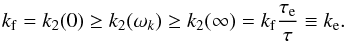 (46)We call ke the elastic Love number. One can consider that the transition between the elastic and the viscous regimes occurs for k2(ω0) = (kf + ke)/2. Because of the expression of k2 (Eq. (45)), we use
  , which gives the very simple transition condition
  (47)If one is able to measure ke, kf and δk for a planet, it becomes possible to determine the relaxation times τ and τe.
4.3. Energy dissipation and orbital evolution
Consider that  , where Ω is constant and δΩ a small perturbation of Ω. Neglecting terms of second order, the rotational energy dissipated in the planet is then easily obtained as
  (48)The variation of orbital energy is obtained as the variation of the potential energy (Eq. (1)) under the variation of the potential coefficients, that is
 ![Mathematical equation: \begin{eqnarray} \dot E_\mathrm{orb} = \M\frac{\partial V}{\partial t} = - \frac{G \M \m R^2}{2a^3}\left[\frac{a^3}{r^3} \dot J_2 + 6\Frac{a^3}{r^3} \, \Re\left( \dot\Z \ep^{{\rm i}2(\lv-\ttheta)}\right)\right] , \end{eqnarray}](/articles/aa/full_html/2014/11/aa24211-14/aa24211-14-eq149.png) (49)where ℜ(z) is the real part of the complex number z. Using the expression of
(49)where ℜ(z) is the real part of the complex number z. Using the expression of  (Eq. (20)) and Sect. 3, we have
  (50)and from expression (35)
 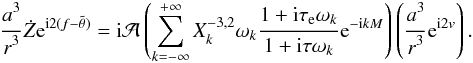 (51)Finally, after averaging over the mean anomaly M,
 ![Mathematical equation: \begin{eqnarray} \langle \dot E_\mathrm{orb} \rangle_M = \frac{C \KK}{6} \sum_{k=-\infty}^{+\infty} \left[ \left(X_k^{-3,0}\right)^2 \! \frac{\taub k^2 n^2 }{1+ \taub^2 k^2 n^2 } + \left(X_k^{-3,2}\right)^2 \!\frac{3 \taub \sig_k^2}{1+ \taub^2 \sig_k^2 } \right] \cdot \end{eqnarray}](/articles/aa/full_html/2014/11/aa24211-14/aa24211-14-eq154.png) (52)The last term results form the contribution of C22 and S22, while the first term results from the contribution of the J2, so it does not depend on the rotation angle (Eq. (20)). We can also easily compute the semi-major axis and eccentricity evolution from the tidal energy (e.g., Correia et al. 2011)
(52)The last term results form the contribution of C22 and S22, while the first term results from the contribution of the J2, so it does not depend on the rotation angle (Eq. (20)). We can also easily compute the semi-major axis and eccentricity evolution from the tidal energy (e.g., Correia et al. 2011) 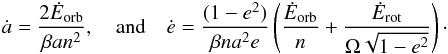 (53)The total energy released inside the body due to tides is then
  (54)A commonly used dimensionless measure of the tidal dissipation is the quality factor,
  (55)where the line integral over Ė is the energy dissipated during one period of tidal stress, and E0 is the peak energy stored in the system during the same period. In general, Q is a function of the frequency ωk, and it can be related to the phase lag through
  (Efroimsky 2012, Eq. (141)). In that case, the ratio k2/Qk is directly connected with the tidal torque (Eq. (43)) and therefore it is easily measurable
 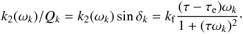 (56)For static perturbations (ωk = 0) the deformation of the planet is maximal (Eq. (45)), but the phase lag δk is zero, so there is no tidal dissipation. All gravity coefficients are given by their equilibrium values (Eqs. (20)−(22)), and the last term in expression (15) and expression (16) become zero. Then, the only effect of the deformation is to add some precession to the elliptical orbit. The same is true for short period perturbations (ωk ≫ 1 /τ), since we also have k2/Qk → 0 (Fig. 2c). However, in this case the equilibrium figure must be corrected using ke instead of kf (Eq. (46)).
5. Equilibrium configurations
5.1. Low frequency regime (| τωk | ≪ 1 for all k)
When τωk ≪ 1 we have  , and the expression of the secular evolution of the rotation rate (41) simplifies. With ωk = 2Ω − kn, and using Appendix B we obtain the following expression for the secular tidal torque
  (57)where Δτ = τ − τe = τv is a constant time-lag between the perturbation and the maximal deformation, that is equivalent to the fluid or “viscous” relaxation time (Eq. (9)),
  (58)and
  (59)Thus, for a given eccentricity, there is only one possible equilibrium configuration for the rotation rate, obtained when T = 0,
  (60)which is often known as the pseudo-synchronization. The low frequency regime is widely described in the literature, and it is usually known as the “viscous” or constant time-lag approximation (e.g., Singer 1968; Alexander 1973; Mignard 1979).
5.2. High frequency regime (τn ≳ 1)
In this case, the situation for equilibrium points (T = 0) is more complex than in the low frequency regime as the expression (41) may have many zeros. The situation is very similar to that discussed for the Andrade rheology model (e.g., Makarov & Efroimsky 2013). Indeed, the torque (Eq. (41)) is a sum  (61)with components of the form
  (62)With Andrade rheology, the torque has an equivalent expression, where all
  are replaced by
  defined as (Efroimsky 2012)
  (63)with
 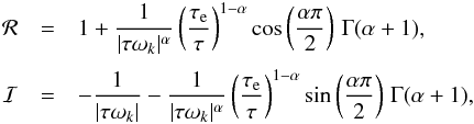 (64)where α is an empirical adjustable parameter whose value depends on the material.
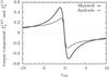 |
Fig. 3 Comparison between Maxwell and Andrade secular tidal torque components Tk. Parameters of Andrade rheology are α = 0.2 and τe/τ = 0.73. |
As shown in Fig. 3, both models have qualitatively similar asymptotic behaviors. Thus, as explained in Makarov & Efroimsky (2013), several spin-orbit resonant configurations are at equilibrium T = 0.
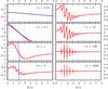 |
Fig. 4 Normalized torque |

In Fig. 4, we show the evolution of the secular tidal torque as τn increases from 1 to 1000 for a given eccentricity e = 0.4. As long as τn ≲ 1, there is only one equilibrium rotation state T = 0 which corresponds to the pseudo-synchronous state. However, as τn increases beyond ~10, around each spin-orbit resonance the torque is dominated by a single component with amplitude  . This leads to many equilibria, but only rotations simultaneously satisfying T = 0 and dT/ dΩ < 0 are stable. As a result, only equilibria close to spin-orbit resonances are stable (Makarov & Efroimsky 2013; Storch & Lai 2014). Moreover, not all spin-orbit configurations are equilibria, since the torque also has to cross the x-axis. This condition is satisfied around a p = k0/ 2 spin-orbit resonance if
 ![Mathematical equation: \begin{eqnarray} {\left[X_{2 p}^{-3,2} (e)\right]^2} \geq 2 \left| \sum_{k=-\infty}^\infty \left[X_k^{-3,2} (e) \right]^2 \frac{\taub\sig_k }{1+\taub^2\sig_k^2} \right| \cdot \label{131105m} \end{eqnarray}](/articles/aa/full_html/2014/11/aa24211-14/aa24211-14-eq198.png) (65)In particular, for the spin-orbit resonance p = 3/2 (the last before the synchronization), by truncating the series for terms equal or higher than e2, we approximately get stability as long as
(65)In particular, for the spin-orbit resonance p = 3/2 (the last before the synchronization), by truncating the series for terms equal or higher than e2, we approximately get stability as long as 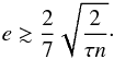 (66)This last expression can also be used to quickly determine which τ values allow non-synchronous rotation for a given eccentricity. In Fig. 5 we plot the critical eccentricities for some spin-orbit resonances as a function of the product τn given by expressions (65) and (66). We conclude that as the relaxation time τ increases, the spin-orbit equilibria are only broken for lower values of the eccentricity, i.e., spin-orbit resonances become more stable.
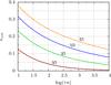 |
Fig. 5 Critical eccentricities for keeping the rotation in a spin-orbit resonance as a function of τn (Eq. (65)). Each color corresponds to a different spin-orbit resonance. The dashed line shows the approximation given by expression (66). Spin-orbit resonances become more stable for higher values of τ. |
6. Libration
Most works on tidal dissipation usually assume the zero order solution in θ, the one in the form  (Sect. 4). However, although the tidal drift on the rotation rate can be neglected over one orbital period, near spin-orbit resonances the rotation may present some libration around the equilibrium configuration. Therefore, we now compute the effect of a low amplitude libration θ1 such that
  (67)with
  , and
, and 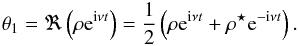 (68)By assumption, the libration amplitude is small: | ρ | ≪ 2π; and the frequency ν is secular. We suppose also that there is an integer k0, for which there is a resonant relation
 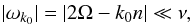 (69)while for all k ≠ k0, | ωk | ≫ ν. In this case, the expression of Ze (Eq. (33)) developped up to the first order in | ρ | reads
 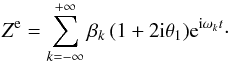 (70)Thus, from Sect. 3, we obtain
 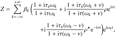 (71)and
 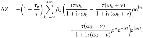 (72)Since (ωk − ωl)t = (k − l)M, from expression (38) for , we obtain at first order in ρ
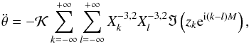 (73)with
 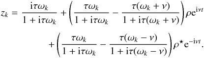 (74)We now average over the mean anomaly M, but keeping the secular libration νt unaveraged, that is
 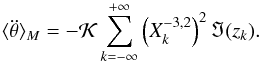 (75)
(75)
6.1. Low libration frequency regime (τν≪ 1)
When τν ≪ 1, the expression (74) can be approximated by  (76)which is exactly the expression without libration. The torque and the evolution of the system are thus identical to those described in Sect. 4.
6.2. High libration frequency regime (τν≫ 1)
Within this regime, it is necessary to distinguish the resonant term from the others. For k ≠ k0, we have | ωk | ≫ ν, and thus expression (74) is again  (77)Conversely, for k = k0, we have | ωk0 | ≪ ν, and expression (74) becomes
  (78)As a result, combining expressions (75), (77), and (78), we get
 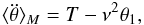 (79)where T is the non-resonant torque (Eq. (41)), and
 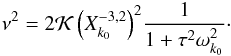 (80)As in the previous section, the non-resonant torque is responsible for the slow variation of Ω, i.e.,
  , and it remains
 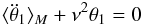 (81)whose solution corresponds to our hypothesis (Eq. (68)).
7. Application to close-in planets
In this section we apply the model described in Sect. 2 to two distinct situations of exoplanets: hot Jupiters and hot super-Earths (Table 1). For that purpose, we numerically integrate the set of Eqs. (15)−(25) for the deformation of the planet, that simultaneously account for orbital and spin evolution due to the rotational flattening and to tides raised by the parent star.
In Table 1 we list the observational parameters for the planets considered in the present study. All these planets were detected through the transiting method combined with radial velocity measurements. Therefore, all orbital parameters are known with good precision, as well as the planetary masses and radius. Thus, the only unknown parameters in the model are the Love numbers (ke and kf) and the relaxation times (τe and τ).
The fluid Love numbers depend on the internal differentiation of the bodies1. In the Solar System we have kf ≈ 0.9 for the terrestrial planets, and 0.3 <kf< 0.5 for the gaseous planets (Yoder 1995). The elastic Love numbers were measured with accuracy only for the Earth and Mars, respectively, ke ≈ 0.3 (Mathews et al. 1995), and ke ≈ 0.15 (Konopliv et al. 2006). For the gaseous planets only the ratio k2/Q is known for Jupiter and Saturn, respectively, k2/Q ≈ 1.1 × 10⁻⁵ (Lainey et al. 2009), and k2/Q ≈ 2.3 × 10⁻⁴ (Lainey et al. 2012). The relaxation times are totally unknown for both terrestrial and gaseous planets, but if one is able to estimate Q, then τ and τe can be estimated through expressions (46) and (56).
Observational data for the planets HD 80606 b (Hébrard et al. 2010), HAT-P-34 b (Bakos et al. 2012), 55 Cnc e (Gillon et al. 2012), and Kepler-78 b (Howard et al. 2013).
7.1. Hot Jupiters
The elastic response of giant gaseous planets is unknown. Since most of the mass is in their huge atmospheres, for simplicity we assume that only the fluid deformation is important, that is, we adopt a purely viscous rheology. We note, however, that the core of these planets also experiences tidal effects, that in some cases can be as strong as those present in the convective envelope (Remus et al. 2012b; Guenel et al. 2014). In addition, other tidal mechanisms, like the excitation of inertial waves, are expected to take place in fluid planets, that also enhance the tidal dissipation (e.g., Ogilvie & Lin 2004; Favier et al. 2014).
In a viscous rheology model, we have τe = 0 and ke = 0. This model is equivalent to the one proposed by Ferraz-Mello (2013), who adopts Q ~ 105 and η ~ 1011 Pa s, and then obtains from expression (7) that τ ~ 1 s. This timescale is intimately connected with the viscous time-lag Δτ = τv between the perturbation and high-tide observed (τv ~ δ/ω, Eq. (44)). Nevertheless, Zahn (1977) has shown that for stars possessing a convective envelope, most of the energy flux is transported by turbulent convection, leading to a strong delay of the equilibrium tide, a “convective viscous time” τc ~ 1 yr, that can be related with the viscous time through (Zahn 1977, Eq. (4.2)) 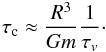 (82)The “convective time” can also be considered for gaseous planets (that is, adopting τ = τc), since they can admit regions of turbulent convection (e.g., Guillot 1999; Ogilvie & Lin 2004). For planets, the effective viscosity of turbulent convection falls rapidly as the oscillation frequency is increased, and in the limit of high tidal frequencies, there is a viscoelastic response to deformation (Ogilvie & Lesur 2012). However, for low tidal frequencies (for instance, a spin-orbit commensurability) some different results should be expected. Therefore, the full deformation of gaseous planets may be on the order of a few years or even decades (for a review see Socrates et al. 2012).
Hot Jupiters are close-in Jupiter-mass planets with orbital periods less than 10 days. The in-situ formation of these planets is unlikely, because of the insufficient disk mass close to the star. The Solar System formation theories suggest that giant planets preferentially form close to the ice-line where water is condensed into ice and the necessary building blocks for the formation of planets could be found in large quantities (e.g., Ida & Lin 2008). Their presence at a close-in orbit can be explained by considering core-accretion simultaneously with disk driven migration (e.g., Lin et al. 1996; Alibert et al. 2005; Mordasini et al. 2009). An alternative explanation is obtained through gravitational interactions with a distant inclined binary companion (e.g., Wu & Murray 2003; Correia et al. 2011) or planet-planet scattering (e.g. Rasio & Ford 1996; Beaugé & Nesvorný 2012) combined with tidal effects. Contrarily to the migration scenario, where the eccentricities are quickly damped to zero, the gravitational interaction mechanism can also explain why some proto-hot Jupiters are still observed with high eccentricity values (e.g., Dawson & Murray-Clay 2013). Since for circular orbits the only possibility for the spin is synchronous rotation (e.g., MacDonald 1964; Hut 1980), in this paper we focus on eccentric planets. The solution for circular orbits is also obtained at the end of the evolution for initially eccentric planets.
Here, we apply our model to the planets HAT-P-34 b (Bakos et al. 2012) and HD 80606 b (Hébrard et al. 2010), both belonging to single-planet systems. The main difference between these two planets is their present orbital period, only 5.45 day for HAT-P-34 b, and about 111 day for HD 80606 b (Table 1). However, due to the angular momentum conservation, when the eccentricity becomes fully damped, the final semi-major axis and orbital period are constrained (e.g., Correia 2009)  (83)This gives 3.94 day and 5.19 day for HAT-P-34 b and HD 80606 b, respectively, that is, both planets will evolve to “regular” hot Jupiter configurations. For HAT-P-34 b we begin our simulations with P = 10.82 day and e = 0.7, while for HD 80606 b we start with the present observed values (Table 1). The initial rotation period is 0.5 day for both planets, and the planet is assumed perfectly spherical (J2 = C22 = S22 = 0). Because the relaxation time is unknown, we adopt different values for τ ranging from 10-5−100 yr, in order to cover all kinds of behavior. For the fluid Love number we use Jupiter’s value kf = 0.5 (Yoder 1995).
In Fig. 6 we show the future evolution of the HD 80606 b orbit (top), rotation (middle) and shape (bottom) using different values of the relaxation time. The shape of the planet is described by its gravity field coefficients. However, since C22 and S22 values constantly change for a non-synchronous planet, we plot the prolateness of the planet,  (84)which is equivalent to the value of C22 along the instantaneous principal long axis of inertia. In all situations, the planet attempts to point the instantaneous long axis to the star, increasing its prolateness until it reaches the pericenter of the orbit. At this stage, the prolateness decreases again, reaching a minima at the apocenter.
 |
Fig. 6 Evolution of HD 80606 b with time for different τ values. We plot the semi-major axis (in AU) and the eccentricity (top), the ratio between the planet rotation rate and the orbital mean motion (middle), and the planet J2 and ϵ (bottom). The green line gives the pseudo-synchronous equilibrium (Eq. (60)) (middle), and the average equilibrium values for J2 and ϵ, respectively (Eqs. (85) and (86)) (bottom). |
For τ = 10-4 yr (Fig. 6, left), the relaxation time is much shorter than the orbital period, so between two consecutive passages at the apocenter, the prolateness of the planet is back to its minimal value. The only effect on the rotation rate is then to decrease it from its initial value, until it reaches the pseudo-synchronous equilibrium (Eq. (60)), since we have τωk ≪ 1 (Sect. 5.1). Because of the conservation of the angular momentum, the eccentricity of the orbit is also progressively damped to zero. When the eccentricity is close to zero, Ω /n ≈ 1 + 6e2 (Eq. (60)), so the equilibrium rotation tends to the synchronous rotation. At this stage the planet is able to acquire a permanent prolateness, always pointing the long axis to the star.
For τ = 10-2 yr (Fig. 6, center), the relaxation time is also shorter than the orbital period during the initial stages of the spin evolution, so the rotation behaves similarly to the previous case (τ = 10-4 yr). However, as the orbit shrinks, the relaxation time and the orbital period become equivalent τn ~ 1. Then, when the planet is back at the pericenter, its prolateness is still excited by the previous pericenter passage. As a consequence, the planet increases its global prolateness at each pericenter passage. This effect is maximized near a spin-orbit commensurability, since the rotation rate is close to a harmonic of the orbital mean motion, Ω /n = p = k0/ 2, and thus there exist one tidal frequency ω2p that is near zero (Sect. 5.2). The gravitational torque exerted by the star on the prolate planet dominates the tidal toque and tends to keep the rotation near the spin-orbit commensurability (Fig. 4). Therefore, in this regime the rotation rate closely follows the spin-orbit equilibria.
Finally, for τ = 1 yr (Fig. 6, right), the relaxation time is permanently larger than the orbital period. Therefore, the prolateness of the planet is continuously excited by a nearby spin-orbit resonance, as explained for the final stages in the previous case. The spin remains trapped in a spin-orbit equilibrium until the eccentricity decreases below a given threshold (Fig. 5). Then, the spin decreases one more step until it is captured in the following lower-order spin-orbit resonance. The process continues until the synchronous equilibrium is reached for small values of the eccentricity, since this is the only spin-orbit resonance that is always stable (Eq. (65)).
For lower and higher τ values the system asymptotically behaves as in the τ = 10-5 yr and 100 yr cases, respectively, the major change is in the evolution timescale, that is longer.
7.2. Evolution versus eccentricity
In Fig. 6, the evolution timescale is different for each τ value, since tidal dissipation is controled by this parameter (Fig. 2). However, because of the conservation of the angular momentum (Eq. (83)), the final semi-major axis is always the same. In addition, there is a perfect correspondence between the semi-major axis and the eccentricity (Fig. 7), that is, the orbital evolution is always the same, only the timescale changes. Therefore, in order to better compare the behavior of the spin with different τ values, instead of using the time, it is preferable to use the semi-major axis or the eccentricity in the evolution axis.
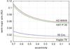 |
Fig. 7 Evolution of the semi-major axis as a function of the eccentricity for different systems and τ values. The dotted lines correspond to the theoretical prediction given by expression (83). Solid lines correspond to the orbital evolution obtained using numerical simulations with different τ values. For each system, the simulations exactly match the theoretical prediction. |
In Fig. 8, we plot the evolution of the spin of HAT-P-34 b and HD 80606 b as a function of the eccentricity for different τ values. The initial rotation period is arbitrarily set at 0.5 day for both planets in all simulations. This value is not critical, because for all τ values the tidal torque on the spin is so strong that the rotation quickly evolves into an equilibrium configuration. We observe that the spin evolution of both planets is identical, although the initial eccentricity of HAT-P-34 is 0.7, while the initial eccentricity of HD 80606 is 0.933. We can also clearly observe the two tidal regimes described in Sect. 5. For low eccentricity values, the orbital period of both planets is around 10-2 yr. Thus, for τ ≪ 10-2 yr, the spin closely follows the pseudo-synchronous equilibrium (Eq. (60)), since τn ≪ 1. For τ ~ 10-2 yr, we observe the transition between regimes, while for τ ≫ 10-2 yr, the spin is captured in half-integer spin-orbit resonances, since τn ≫ 1. These resonances become destabilized as the eccentricity decays, in agreement with expression (65). The main consequence of these metastable equilibria is to allow faster rotation rates for an identical eccentricity.
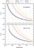 |
Fig. 8 Evolution of the rotation rate as a function of the eccentricity for different τ values (10-5 ≤ τ ≤ 100 yr). The initial rotation period is 0.5 day for both planets, but this value is not critical as the spin quickly evolves to an equilibrium configuration. For τ< 10-3 yr, the spin closely follows the pseudo-synchronous equilibrium (Eq. (60)). For τ> 10-2 yr, the spin is captured in half-integer spin-orbit resonances that become destabilized as the eccentricity decays, in agreement with expression (65). |
In Fig. 9, we plot the evolution of the shape (J2 and ϵ) of HD 80606 b as a function of the eccentricity. To better understand the different behaviors, we also plot the average of the equilibrium shape over one orbital period (Eqs. (20)−(22))
![Mathematical equation: \begin{eqnarray} \label{140103b}&&\left\langle J_2 \right\rangle_M = \kf \left[ \frac{\om^2 R^3}{3 G \m} + \frac{1}{2} \frac{\M}{\m} \left(\frac{R}{a} \right)^3 \left(1-e^2\right)^{-3/2} \right], \\ \label{140103c}&&\left\langle \epsilon \right\rangle_M = \frac{\kf}{4} \frac{\M}{\m} \left(\frac{R}{a}\right)^3 \left(1-e^2\right)^{-3/2}, \end{eqnarray}](/articles/aa/full_html/2014/11/aa24211-14/aa24211-14-eq285.png) as well as the equilibrium shape for a planet trapped in a specific spin-orbit resonance p = k0/ 2 (Eq. (33))
as well as the equilibrium shape for a planet trapped in a specific spin-orbit resonance p = k0/ 2 (Eq. (33)) 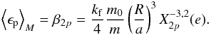 (87)For τ ≪ 10-2 yr, J2 and ϵ present large oscillations around the average equilibrium shape (Eqs. (85) and (86)). The maximal value corresponds to the equilibrium shape at the pericenter, while the minimal value corresponds to the equilibrium shape at the apocenter, obtained by replacing r = a(1 − e) and r = a(1 + e) in expressions (20) to (22), respectively. In this regime the relaxation time is much shorter than the orbital period, so the figure of the planet is almost equal to the instantaneous equilibrium figure.
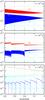 |
Fig. 9 Evolution of J2 (in red) and prolateness ϵ (in blue) of HD 80606 b as a function of the eccentricity for different τ values. The green dashed line shows the average equilibrium value of these two quantities over one orbital period (Eqs. (85), (86)). The cyan dashed line shows the average equilibrium value of the prolateness for a specific spin-orbit resonance (Eq. (87)). |
For τ ≫ 10-2 yr, the relaxation time is much longer than the orbital period, so it is possible to temporary lock the spin in resonance. Therefore, the J2 of the planet closely follows the average equilibrium value (Eq. (85)), although sudden variations are observed, corresponding to the transition between two spin-orbit resonances. The prolateness of the planet also follows the equilibrium value for each spin-orbit resonance (Eq. (87)). The prolateness temporarily decreases with the eccentricity, since  is a decreasing function with e (check Table C.1). However, when the critical eccentricity for each resonance is attained (Eq. (65)), the prolateness ϵ increases again stabilizing in the following resonance.
For τ = 10-2 yr, we observe a mix of both behaviors mentioned above. The prolateness ϵ still follows the resonant equilibrium values (Eq. (87)), but now presents significant oscillations around it. Resonances also become unstable for higher eccentricity values in agreement with Fig. 5. Finally, at the end of the evolution (e = 0), the planet always evolves into the synchronous resonance, acquiring the same J2 and ϵ value in all scenarios.
7.3. Super-Earths
In general, a super-Earth is defined exclusively by its mass, independently of its environment being similar to that of the Earth. An upper bound of 10 Earth masses is commonly accepted to warrant that the planet is mostly rocky (e.g., Valencia et al. 2007). Therefore, the rheology of these planets is expected to be similar to the terrestrial planets in the Solar System. We adopt here the full viscoelastic model described in Sect. 2, using the Earth’s values for the Love numbers, ke = 0.3 and kf = 0.9 (Yoder 1995).
For the Earth and Mars, we have Q = 10 (Dickey et al. 1994) and Q = 80 (Lainey et al. 2007), respectively. We then compute for the Earth τ = 1.6 day and τe = 0.5 day, and for Mars τ = 14.7 day and τe = 2.5 day. However, in the case of the Earth, the present Q-factor is dominated by the oceans, the Earth’s solid body Q is estimated to be 280 (Ray et al. 2001), which increases the relaxation time by more than one order of magnitude (τ = 46 day and τe = 15 day). Although these values provide a good estimation for the average present dissipation ratios, they appear to be incoherent with the observed deformation of the planets. Indeed, in the case of the Earth, the surface post-glacial rebound due to the last glaciation about 104 years ago is still going on, suggesting that the Earth’s mantle relaxation time is something like τ = 4400 year (Turcotte & Schubert 2002). Therefore, we conclude that the deformation of terrestrial planets can range from a few days up to thousands of years.
Here we apply our model to the planets 55 Cnc e (Gillon et al. 2012) and Kepler-78 b (Howard et al. 2013). The main difference between these two planets is their masses, only 1.7 M⊕ for Kepler-78 b, and about 8.6 M⊕ for 55 Cnc e (Table 1). 55 Cnc e belongs to a multi-planet system, but in the present study we ignore the gravitational interactions with the remaining companions, as in Rodríguez et al. (2012). Contrary to hot Jupiters from the previous section, the present eccentricities of these two super-Earths are very small, nearly zero. Therefore, as for HAT-P-34 b, we begin our simulations with e = 0.7, so that we can observe some tidal evolution. The initial orbital periods are obtained through expression (83), which gives about 0.97 and 2.05 day for Kepler-78 b and 55 Cnc e, respectively. Because the relaxation time is unknown and can vary by some orders of magnitude, we adopt different values for τ ranging from 10-2−101 yr.
The initial rotation period is arbitrarily set at 0.5 day for both planets in all simulations. This value is not critical, because for all τ values the tidal torque on the spin is so strong that the spin quickly evolves into a spin-orbit resonance (Figs. 10 and 11). Since the initial orbital period is only ~1 day, we get Ω ~ n from the beginning of the simulations. For instance, in the case of 55 Cnc e we have Ω /n ≈ 4.1, that is, the spin starts close to the 4/1 spin-orbit resonance. However, the initial planet is assumed perfectly spherical (J2 = C22 = S22 = 0), so during the initial stages of the evolution (on the order of τ), the spin is chaotic, until the gravity field coefficients acquire some stable deformation. As a consequence, the spin can be stabilized in spin-orbit resonances different from the 4/1, depending on the initial phase of the rotation angle θ (Fig. 10). Although the initial capture in a spin-orbit resonance is random, the subsequent evolution is very predictable: as the eccentricity decreases, the higher-order resonances become unstable, and the spin successively quits them one by one, until it reaches the synchronous rotation at the end of the evolution.
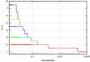 |
Fig. 10 Evolution of the rotation of 55 Cnc e as a function of the eccentricity for different initial θ values and τ = 101 yr. The initial rotation rate is Ω /n ≈ 4.1, but since the initial shape of the planet is perfectly spherical (J2 = C22 = S22 = 0), the initial rotation is chaotic and the spin may be trapped in different spin-orbit resonances. As the eccentricity decreases, the higher-order resonances become unstable, and the spin successively quits them, until it reaches the synchronous rotation. |
In Fig. 11, we plot the evolution of the spin as a function of the eccentricity for different τ values. Unlike hot Jupiters, for the considered τ values (and higher), super-Earths are always found in the high-frequency tidal regime (Sect. 5.2). Therefore, the spin is always captured in a spin-orbit resonance, and subsequently evolves to lower-order resonances as the eccentricity decreases. For higher τ values, the resonances become more stable, in agreement with expression (65), so the planet requires a lower eccentricity value before reaching the synchronous rotation. For planets in multi-body systems like 55 Cnc e, we cannot rule out a non-synchronous rotation at present. Using the observed value of e = 0.057 in expression (66), we conclude that 55 Cnc e is only synchronous if τ< 10-2 yr (Fig. 11).
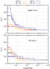 |
Fig. 11 Evolution of the rotation rate as a function of the eccentricity for different τ values (10-2 ≤ τ ≤ 101 yr). The initial rotation period is 0.5 day for both planets, but this value is not critical as the spin quickly evolves into a spin-orbit resonance (Fig. 10). The resonances are destabilized as the eccentricity decays, in agreement with expression (65). |
In Fig. 12, we plot the evolution of the shape (J2 and ϵ) of 55 Cnc e as a function of the eccentricity. As for hot Jupiters (Fig. 9), we also plot the average of J2 over one orbital period of the equilibrium (Eq. (85)), as well as the average of ϵ for a planet trapped in a specific spin-orbit resonance ![Mathematical equation: \begin{eqnarray} \left\langle \epsilon_{\rm p} \right\rangle_M = \frac{\kf}{4} \frac{\M}{\m} \left(\frac{R}{a}\right)^3 \left[ \left(1-\frac{\taua}{\taub} \right) \, X_{2p}^{-3,2} (e) + \frac{\taua}{\taub} \left(1-e^2\right)^{-3/2} \right] . \label{140107a} \end{eqnarray}](/articles/aa/full_html/2014/11/aa24211-14/aa24211-14-eq312.png) (88)This expression is different from its analog for hot Jupiters (Eq. (87)), because here we have an elastic contribution to ϵ, while previously we only considered the viscous contribution (τe = 0). This equilibrium is also independent of the relaxation times, since τe/τ = ke/kf (Eq. (46)) (in our simulations τe/τ = 1/3).
(88)This expression is different from its analog for hot Jupiters (Eq. (87)), because here we have an elastic contribution to ϵ, while previously we only considered the viscous contribution (τe = 0). This equilibrium is also independent of the relaxation times, since τe/τ = ke/kf (Eq. (46)) (in our simulations τe/τ = 1/3).
For all τ> 10-2 yr, the J2 of the planet closely follows the average of the equilibrium value (Eq. (85)), the sudden variations corresponding to the transition between two spin-orbit resonances. The prolateness of the planet also follows the equilibrium value for each spin-orbit resonance (Eq. (88)). However, for all spin-orbit resonances different from the synchronization, the elastic contribution given by the second term in expression (88) is dominating (in particular for low eccentricity values), since for p ≠ 1 we have  (Table C.1). Thus, for all these resonances the observed prolateness converges to the same equilibrium value,
  (89)For the synchronous resonance, we have
  (Table C.1), so both terms in expression (88) add up to give an equilibrium identical to the previous one (Eq. (89)), but where τe and ke are replaced by τ and kf, respectively. This final equilibrium for ϵ is exactly the same as for hot Jupiters (Eq. (87)).
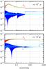 |
Fig. 12 Evolution of J2 (in red) and prolateness ϵ (in blue) of 55 Cnc e as a function of the eccentricity for different τ values. The green dashed line shows the average equilibrium value of J2 over one orbital period (Eq. (85)). The cyan dashed line shows the average equilibrium value of the prolateness for each spin-orbit resonance (Eq. (88)). |
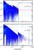 |
Fig. 13 Evolution of the “permanent” prolateness (in blue) of 55 Cnc e as a function of the eccentricity for different τ values. The cyan dashed lines show the average equilibrium value of the “permanent” prolateness for each spin-orbit resonance (first term in Eq. (88)). The pink dashed lines give the strength of the tidal torque for each resonance (Eq. (41)). |
Despite ϵ has a dominating “elastic” contribution, the first term in expression (88) corresponds to a “permanent” deformation. That is, while the deformation that results from the contribution of the first term is along an axis that is fixed with respect to the body, the deformation resulting from the second term nearly points to the direction of the star. As a result, only the “permanent” contribution is responsible for the capture in resonance. In Fig. 13 we show the evolution of the “permanet” prolateness with the eccentricity, i.e., we show ϵ subtracted from its “elastic” term (Eq. (89)). As expected, the “permanent” prolateness closely follows the equilibrium cyan dashed lines given by the first term in expression (88).
In Fig. 13, we additionally plot in pink dashed lines the strength of the tidal torque for each spin-orbit resonance (Eq. (41)). We observe that the equilibrium in each resonance is broken exactly when the cyan and pink dashed lines intercept. This result is in perfect agreement with the theoretical prediction from expression (65), and confirms that only the “permanent” contribution to ϵ is responsible for the capture in resonance.
8. Conclusions
In this paper we presented a new approach to the tidal theory. Adopting the same strategy as Darwin (1879), we are able to extend the creep equation obtained for a homogeneous incompressible viscous body to also include the elastic rebound. The deformation law hence obtained (Eq. (9)) corresponds to the deformation of a Maxwell material. The deformation is then taken into account by means of the effect of the disturbing potential on the gravity field coefficients of the planet (Eq. (14)). This method allows us to easily compute the instantaneous variations in the shape of the planet when subject to a perturbation.
In this study we considered the planar case, where the spin of the planet is orthogonal to its orbit. The planet is deformed under the effect of tidal perturbations, but also by the changes in its rotation due to the centrifugal potential. Our model can be easily extended to non-planar configurations (for planets with some obliquity and evolving in inclined orbits), provided that we additionally take into account the deformation of the C21 and S21 gravity field coefficients in the gravitational potential (Eq. (1)), as explained in Correia & Rodríguez (2013).
There are several advantages in using our model. First, it works for any kind of perturbation, even for the non-periodic ones (such as chaotic motions or transient events). Thus, we no longer need to decompose the tidal potential in an infinite sum of harmonics of the tidal frequency (e.g., Kaula 1964; Mathis & Le Poncin-Lafitte 2009; Efroimsky & Williams 2009). Second, as long as we can neglect terms in (R/r)3, the model is valid for any eccentricity value, we do not need to truncate the equations of motion. Finally, it simultaneously reproduces the deformation and the dissipation on the planet. This last point is very important, because it clarifies an important behavior of the tidal torque: its ability to temporarily lock the planet in a spin-orbit resonance. Indeed, for relaxation times longer than the orbital period (τn ≫ 1), when the planet is back at the pericenter, its shape is still excited by the previous pericenter passage. The planet thus increases its global prolateness at each pericenter passage, an effect that is maximized near a spin-orbit commensurability. The gravitational torque exerted by the star on the prolate planet dominates the tidal torque and tends to keep the rotation near the spin-orbit commensurability (Fig. 4).
Another important outcome of our study is that gaseous planets can also present non-synchronous spin-orbit equilibria. The only requirement is that the relaxation time is longer than the orbital period. Although this seems unlikely for the gaseous envelop, giant planets also contain liquid and solid cores that may take longer to acquire their equilibrium shape (e.g., Remus et al. 2012b; Auclair-Desrotour et al. 2014). In particular, we cannot rule out this possibility for hot Jupiters, since they have very short orbital periods.
For close-in super-Earths (or terrestrial planets), the relaxation time of the mantle is almost certainly longer than the orbital period. As a consequence, our model shows that the rotation is temporarily locked in several spin-orbit resonances throughout the evolution. These equilibria are destabilized as the eccentricity decreases, but non-synchronous rotation can be maintained even for extremely low eccentricity values, depending on the relaxation time. Moreover, if there are other planetary companions, the eccentricity is never exactly zero (e.g., Laskar et al. 2012), so the higher-order spin-orbit resonances can be maintained for the entire life of the system. As a consequence, we expect that in many cases, the rotation of close-in terrestrial planets in multi-planet systems is captured in non-synchronous spin-orbit resonances.
Our model is also able to reproduce the results by Ferraz-Mello (2013) for a Newtonian creep. For that, we just need to set τ = γ-1 and τe = 0, and thus neglect expressions (23−25). Actually, apart from the elastic deformation of the planet, this simplification still allows us to reproduce the main features described in this paper, like the different regimes of dissipation and the spin-orbit capture. Therefore, for studies where the deformation of the planet does not matter (i.e., only the dissipation is relevant), we can adopt the above simplification using a modified Love number  instead of kf (Eq. (56))
 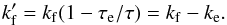 (90)Remus et al. (2012b) have shown that for a planet composed of a homogeneous core surrounded by a fluid envelope of constant density (which can be a rocky planet with a deep non-dissipative ocean, or a giant planet with a solid core), the global response to the perturbations can be modeled by a viscoelastic rheology. As an illustration, they present the results for a Maxwell body. Thus, our model can also be used to study planets with more complex structures, provided that we use modified Love numbers. In addition, we can generalize it to other rheologies. In order to determine the specific deformation law that replaces expression (9), one just needs to know how the strain is related to the stress in each case (see Appendix A). However, in the case of complex rheologies, this method may lead to a differential system of very high order, that is less easy to handle.
The inclusion of general relativity or the effect from an oblate star would result in a correction to the precession rate of the pericenter,  (e.g., Correia et al. 2011). Since the rotation rate is defined as
  (Eq. (34)), these effects do not modify the conclusions and the results reported in this paper.
The fluid Love numbers depend on the internal differentiation of the bodies. For a homogeneous incompressible viscous sphere we have hf = 5/2 and kf = hf−1 = 3/2, but more generally the fluid Love numbers can be obtained from the Darwin-Radau equation (e.g., Jeffreys 1976): hf = 5(1 + [ 5/2−15C/ (4mR2) ] 2)-1.
Acknowledgments
We acknowledge support from the PNP-CNRS, CS of Paris Observatory, PICS05998 France-Portugal program, FCT-Portugal (PEst-C/CTM/LA0025/2011), and FAPESP-Brazil (2009/16900-5, 2012/13731-0).
References
- Adel Sharaf, M., & Hassan Selim, H. 2010, Research in Astronomy and Astrophysics, 10, 1298 [NASA ADS] [CrossRef] [Google Scholar]
- Alexander, M. E. 1973, Ap&SS, 23, 459 [NASA ADS] [CrossRef] [Google Scholar]
- Alibert, Y., Mordasini, C., Benz, W., & Winisdoerffer, C. 2005, A&A, 434, 343 [NASA ADS] [CrossRef] [EDP Sciences] [Google Scholar]
- Andrade, E. N. D. C. 1910, Proc. R. Soc. London, A, 84, 1 [Google Scholar]
- Auclair-Desrotour, P., Le Poncin-Lafitte, C., & Mathis, S. 2014, A&A, 561, L7 [NASA ADS] [CrossRef] [EDP Sciences] [Google Scholar]
- Bakos, G. Á., Hartman, J. D., Torres, G., et al. 2012, AJ, 144, 19 [NASA ADS] [CrossRef] [Google Scholar]
- Beaugé, C., & Nesvorný, D. 2012, ApJ, 751, 119 [NASA ADS] [CrossRef] [Google Scholar]
- Colombo, G. 1965, Nature, 208, 575 [NASA ADS] [CrossRef] [Google Scholar]
- Correia, A. C. M. 2009, ApJ, 704, L1 [NASA ADS] [CrossRef] [Google Scholar]
- Correia, A. C. M., & Rodríguez, A. 2013, ApJ, 767, 128 [NASA ADS] [CrossRef] [Google Scholar]
- Correia, A. C. M., Laskar, J., Farago, F., & Boué, G. 2011, Celest. Mech. Dyn. Astron., 111, 105 [Google Scholar]
- Darwin, G. H. 1879, Philos. Trans. R. Soc. London, 170, 1 [Google Scholar]
- Darwin, G. H. 1880, Philos. Trans. R. Soc. London, 171, 713 [NASA ADS] [CrossRef] [Google Scholar]
- Dawson, R. I., & Murray-Clay, R. A. 2013, ApJ, 767, L24 [NASA ADS] [CrossRef] [Google Scholar]
- Dickey, J. O., Bender, P. L., Faller, J. E., et al. 1994, Science, 265, 482 [NASA ADS] [CrossRef] [PubMed] [Google Scholar]
- Efroimsky, M. 2012, Celest. Mech. Dyn. Astron., 112, 283 [NASA ADS] [CrossRef] [Google Scholar]
- Efroimsky, M., & Williams, J. G. 2009, Celest. Mech. Dyn. Astron., 104, 257 [Google Scholar]
- Favier, B., Barker, A. J., Baruteau, C., & Ogilvie, G. I. 2014, MNRAS, 439, 845 [NASA ADS] [CrossRef] [Google Scholar]
- Ferraz-Mello, S. 2013, Celest. Mech. Dyn. Astron., 116, 109 [NASA ADS] [CrossRef] [Google Scholar]
- Gillon, M., Demory, B.-O., Benneke, B., et al. 2012, A&A, 539, A28 [NASA ADS] [CrossRef] [EDP Sciences] [Google Scholar]
- Goldreich, P., & Peale, S. 1966, AJ, 71, 425 [NASA ADS] [CrossRef] [Google Scholar]
- Guenel, M., Mathis, S., & Remus, F. 2014, A&A, 566, L9 [NASA ADS] [CrossRef] [EDP Sciences] [Google Scholar]
- Guillot, T. 1999, Science, 286, 72 [NASA ADS] [CrossRef] [PubMed] [Google Scholar]
- Hébrard, G., Désert, J.-M., Díaz, R. F., et al. 2010, A&A, 516, A95 [NASA ADS] [CrossRef] [EDP Sciences] [Google Scholar]
- Henning, W. G., O’Connell, R. J., & Sasselov, D. D. 2009, ApJ, 707, 1000 [NASA ADS] [CrossRef] [Google Scholar]
- Howard, A. W., Sanchis-Ojeda, R., Marcy, G. W., et al. 2013, Nature, 503, 381 [NASA ADS] [CrossRef] [Google Scholar]
- Hughes, S. 1981, Cel. Mech., 25, 101 [Google Scholar]
- Hut, P. 1980, A&A, 92, 167 [NASA ADS] [Google Scholar]
- Ida, S., & Lin, D. N. C. 2008, ApJ, 685, 584 [NASA ADS] [CrossRef] [Google Scholar]
- Jeffreys, H. 1976, The earth. Its origin, history and physical constitution (Cambridge: Cambridge University Press) [Google Scholar]
- Kant, I. 1754, Kant’s cosmogony: As in his essay on the retardation of the rotation of the earth and his Natural history and theory of the heavens (General books) [Google Scholar]
- Kaula, W. M. 1964, Rev. Geophys., 2, 661 [Google Scholar]
- Kelvin, W. T. B. 1863a, Philos. Trans. Roy. Soc. Lond., 153, 583 [Google Scholar]
- Kelvin, W. T. B. 1863b, Philos. Trans. Roy. Soc. Lond., 153, 573 [CrossRef] [Google Scholar]
- Konopliv, A. S., Yoder, C. F., Standish, E. M., Yuan, D.-N., & Sjogren, W. L. 2006, Icarus, 182, 23 [NASA ADS] [CrossRef] [Google Scholar]
- Lainey, V., Dehant, V., & Pätzold, M. 2007, A&A, 465, 1075 [NASA ADS] [CrossRef] [EDP Sciences] [Google Scholar]
- Lainey, V., Arlot, J.-E., Karatekin, Ö., & van Hoolst, T. 2009, Nature, 459, 957 [NASA ADS] [CrossRef] [PubMed] [Google Scholar]
- Lainey, V., Karatekin, Ö., Desmars, J., et al. 2012, ApJ, 752, 14 [NASA ADS] [CrossRef] [Google Scholar]
- Laskar, J., & Boué, G. 2010, A&A, 522, A60 [NASA ADS] [CrossRef] [EDP Sciences] [Google Scholar]
- Laskar, J., Boué, G., & Correia, A. C. M. 2012, A&A, 538, A105 [NASA ADS] [CrossRef] [EDP Sciences] [Google Scholar]
- Lin, D. N. C., Bodenheimer, P., & Richardson, D. C. 1996, Nature, 380, 606 [NASA ADS] [CrossRef] [Google Scholar]
- Love, A. E. H. 1911, Some Problems of Geodynamics (Cambridge: Cambridge University Press) [Google Scholar]
- MacDonald, G. J. F. 1964, Revs. Geophys., 2, 467 [CrossRef] [Google Scholar]
- Makarov, V. V., & Efroimsky, M. 2013, ApJ, 764, 27 [NASA ADS] [CrossRef] [Google Scholar]
- Mathews, P. M., Buffet, B. A., & Shapiro, I. I. 1995, Geophys. Res. Lett., 22, 579 [NASA ADS] [CrossRef] [Google Scholar]
- Mathis, S., & Le Poncin-Lafitte, C. 2009, A&A, 497, 889 [NASA ADS] [CrossRef] [EDP Sciences] [Google Scholar]
- Mignard, F. 1979, Moon and Planets, 20, 301 [Google Scholar]
- Mordasini, C., Alibert, Y., & Benz, W. 2009, A&A, 501, 1139 [NASA ADS] [CrossRef] [EDP Sciences] [Google Scholar]
- Newton, I. 1760, PhilosophiæNaturalis Principia Mathematica (Colonia: A. Philbert) [Google Scholar]
- Ogilvie, G. I., & Lesur, G. 2012, MNRAS, 422, 1975 [NASA ADS] [CrossRef] [Google Scholar]
- Ogilvie, G. I., & Lin, D. N. C. 2004, ApJ, 610, 477 [NASA ADS] [CrossRef] [Google Scholar]
- Rasio, F. A., & Ford, E. B. 1996, Science, 274, 954 [NASA ADS] [CrossRef] [PubMed] [Google Scholar]
- Ray, R. D., Eanes, R. J., & Lemoine, F. G. 2001, Geophys. J. Int., 144, 471 [NASA ADS] [CrossRef] [Google Scholar]
- Remus, F., Mathis, S., & Zahn, J.-P. 2012a, A&A, 544, A132 [NASA ADS] [CrossRef] [EDP Sciences] [Google Scholar]
- Remus, F., Mathis, S., Zahn, J.-P., & Lainey, V. 2012b, A&A, 541, A165 [NASA ADS] [CrossRef] [EDP Sciences] [Google Scholar]
- Rodríguez, A., Callegari, N., Michtchenko, T. A., & Hussmann, H. 2012, MNRAS, 427, 2239 [NASA ADS] [CrossRef] [Google Scholar]
- Singer, S. F. 1968, Geophys. J. R. Astron. Soc., 15, 205 [CrossRef] [Google Scholar]
- Socrates, A., Katz, B., & Dong, S. 2012 [arXiv:1209.5724] [Google Scholar]
- Storch, N. I., & Lai, D. 2014, MNRAS, 438, 1526 [CrossRef] [Google Scholar]
- Turcotte, D. L., & Schubert, G. 2002, Geodynamics (Cambridge: Cambridge University Press) [Google Scholar]
- Valencia, D., Sasselov, D. D., & O’Connell, R. J. 2007, ApJ, 656, 545 [Google Scholar]
- Wu, Y., & Murray, N. 2003, ApJ, 589, 605 [NASA ADS] [CrossRef] [EDP Sciences] [Google Scholar]
- Yoder, C. F. 1995, in Global Earth Physics: A Handbook of Physical Constants (Washington: American Geophysical Union), 1 [Google Scholar]
- Zahn, J.-P. 1977, A&A, 57, 383 [NASA ADS] [Google Scholar]
Appendix A: Fourier domain
A planet with mass m and radius R placed in a static external quadrupolar gravitational potential Vp(r) deforms itself until it reaches a hydrostatic equilibrium. In turn, this deformation generates an additional gravitational potential V′(r). For a homogeneous incompressible elastic solid body, the additional potential is given on the planet’s surface by (Kelvin 1863a,b; Love 1911)  (A.1)where k2 is the second Love number associated with a static perturbing potential. It is related to the rigidity μ of the planet through (Kelvin 1863a,b; Love 1911)
  (A.2)According to the correspondence principle, in the more general case where the external gravitational potential is not static, expression (A.1) remains the same in the Fourier domain (Darwin 1879; Efroimsky 2012, and references therein), and thus
 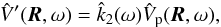 (A.3)where ω is a frequency, and
 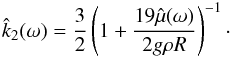 (A.4)In the case of a viscoelastic material characterized by Maxwell rheology – represented at the mesoscopic scale by a spring with elastic modulus μ and a damper with viscosity η put in parallel – the strain ε is related to the stress σ through the differential equation
 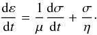 (A.5)The expression of
  is then obtained by performing a Fourier transform on (A.5), which leads to
 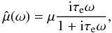 (A.6)with τe = η/μ being the Maxwell relaxation time. Equations (A.3), (A.4), and (A.6), are then combined together to get (e.g., Henning et al. 2009)
  (A.7)where kf = 3/2 is the fluid second Love number and
  (A.8)In a last step, we convert (A.7) into a differential equation in the temporal domain by multiplying both sides by 1 + iτω and substituting “iω” by “d/dt”. The result is
  (A.9)
(A.9)
Appendix B: Linear model
The secular evolution of the rotation rate is given by (Eq. (41)) ![Mathematical equation: \appendix \setcounter{section}{2} \begin{eqnarray} \left\langle \ddot \theta \right\rangle_M = - \kf \frac{3 G \M^2 R^5}{2 C a^6} \sum^{+\infty}_{k=-\infty} \left[ X_k^{-3,2} (e) \right]^2 \frac{(\taub-\taua)\sig_k}{1 + \taub^2\sig_k^2} , \label{eq.torque} \end{eqnarray}](/articles/aa/full_html/2014/11/aa24211-14/aa24211-14-eq347.png) (B.1)In the low frequency regime (τωk ≪ 1), using ωk = 2Ω − kn and Δτ = τ − τe, we can rewrite previous expression as
(B.1)In the low frequency regime (τωk ≪ 1), using ωk = 2Ω − kn and Δτ = τ − τe, we can rewrite previous expression as ![Mathematical equation: \appendix \setcounter{section}{2} \begin{eqnarray} \left\langle \ddot \theta \right\rangle_M &=& - \kf \frac{3 G \M^2 R^5}{2 C a^6} \sum^{+\infty}_{k=-\infty} \left[ X_k^{-3,2} (e) \right]^2 \Delta \tau \, (2\om-kn) \crm &=& - \kf \frac{3 G \M^2 R^5}{C a^6} n \Delta \tau \left(f_1(e) \frac{\om}{n} - f_2(e)\right) , \label{eq.torque2} \end{eqnarray}](/articles/aa/full_html/2014/11/aa24211-14/aa24211-14-eq351.png) (B.2)where
(B.2)where ![Mathematical equation: \appendix \setcounter{section}{2} \begin{eqnarray} f_1(e) = \sum^{+\infty}_{k=-\infty} \left[ X_k^{-3,2} (e) \right]^2 , \end{eqnarray}](/articles/aa/full_html/2014/11/aa24211-14/aa24211-14-eq352.png) (B.3)and
(B.3)and ![Mathematical equation: \appendix \setcounter{section}{2} \begin{eqnarray} f_2(e) = \frac{1}{2} \sum^{+\infty}_{k=-\infty} k \left[ X_k^{-3,2} (e) \right]^2. \end{eqnarray}](/articles/aa/full_html/2014/11/aa24211-14/aa24211-14-eq353.png) (B.4)We let
(B.4)We let  (B.5)Using the definition of the Hansen coefficients (Eq. (32)), we get
 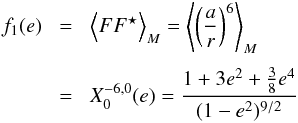 (B.6)and
 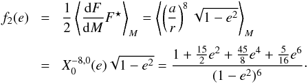 (B.7)The expressions for
  and
and  can be found in (e.g., Laskar & Boué 2010).
Appendix C: Hansen coefficients
The construction of Figs. 4 and 5, requires the computation of many Hansen coefficients (Eqs. (61) and (65)). These coefficients can be efficiently computed using Fourier techniques. The functions  are 2π-periodic functions of mean anomaly M. They can thus be developed in Fourier series with integer frequencies k ∈Z. The corresponding Fourier coefficients are precisely the Hansen coefficients
  . Using this property, it is possible to get at once a numerical estimate of 2N + 1 Hansen coefficients for − K ≤ k ≤ K with K = 2N − 1 by means of a fast Fourier transform (FFT) (Adel Sharaf & Hassan Selim 2010). For that purpose, each function Fl,m(M) has to be evenly sampled in an array y[0:2N − 1] of size 2N − 1 with y[j]:= Fl,m(Mj) where
  (C.1)and j = 0,...,2N − 1. Then, the output y_FFT[0:2N − 1] of the FFT algorithm contains 2N − 1 Hansen coefficients. If the jth term y_FFT[j] is associated with the frequency ωj = j, the Hansen coefficients are sorted in the following order
  (C.2)The last coefficient is deduced from
  . In Table C.1 we list the Hansen coefficients
  up to e6, that appear often throughout this paper.
Hansen coefficients up to e6.
All Tables
Observational data for the planets HD 80606 b (Hébrard et al. 2010), HAT-P-34 b (Bakos et al. 2012), 55 Cnc e (Gillon et al. 2012), and Kepler-78 b (Howard et al. 2013).
All Figures
|
Fig. 1 Reference angles and notations. (i,j,k) is a fixed inertial reference frame, while (I,J,K) is a reference frame fixed in the planet. k = K are orthogonal to the orbit, and thus not shown. r is the radius vector from m to m0, P is the direction of pericenter, ϖ is the longitude of pericenter, and v is the true anomaly. The rotation angle θ is referred to the fixed reference direction i. We also use the angles |
| In the text | |
|
Fig. 2 Evolution of the second Love number k2, the dissipation Q-factor, and phase lag k2sinδ as a function of the tidal frequency ω (normalized by the relaxation time τ). For all parameters there is a transition of regime around τω ~ 1. We use here the Earth values for the Love numbers, ke = 0.3 and kf = 0.9 (Yoder 1995). |
| In the text | |
|
Fig. 3 Comparison between Maxwell and Andrade secular tidal torque components Tk. Parameters of Andrade rheology are α = 0.2 and τe/τ = 0.73. |
| In the text | |
|
Fig. 4 Normalized torque |
| In the text | |
|
Fig. 5 Critical eccentricities for keeping the rotation in a spin-orbit resonance as a function of τn (Eq. (65)). Each color corresponds to a different spin-orbit resonance. The dashed line shows the approximation given by expression (66). Spin-orbit resonances become more stable for higher values of τ. |
| In the text | |
|
Fig. 6 Evolution of HD 80606 b with time for different τ values. We plot the semi-major axis (in AU) and the eccentricity (top), the ratio between the planet rotation rate and the orbital mean motion (middle), and the planet J2 and ϵ (bottom). The green line gives the pseudo-synchronous equilibrium (Eq. (60)) (middle), and the average equilibrium values for J2 and ϵ, respectively (Eqs. (85) and (86)) (bottom). |
| In the text | |
|
Fig. 7 Evolution of the semi-major axis as a function of the eccentricity for different systems and τ values. The dotted lines correspond to the theoretical prediction given by expression (83). Solid lines correspond to the orbital evolution obtained using numerical simulations with different τ values. For each system, the simulations exactly match the theoretical prediction. |
| In the text | |
|
Fig. 8 Evolution of the rotation rate as a function of the eccentricity for different τ values (10-5 ≤ τ ≤ 100 yr). The initial rotation period is 0.5 day for both planets, but this value is not critical as the spin quickly evolves to an equilibrium configuration. For τ< 10-3 yr, the spin closely follows the pseudo-synchronous equilibrium (Eq. (60)). For τ> 10-2 yr, the spin is captured in half-integer spin-orbit resonances that become destabilized as the eccentricity decays, in agreement with expression (65). |
| In the text | |
|
Fig. 9 Evolution of J2 (in red) and prolateness ϵ (in blue) of HD 80606 b as a function of the eccentricity for different τ values. The green dashed line shows the average equilibrium value of these two quantities over one orbital period (Eqs. (85), (86)). The cyan dashed line shows the average equilibrium value of the prolateness for a specific spin-orbit resonance (Eq. (87)). |
| In the text | |
|
Fig. 10 Evolution of the rotation of 55 Cnc e as a function of the eccentricity for different initial θ values and τ = 101 yr. The initial rotation rate is Ω /n ≈ 4.1, but since the initial shape of the planet is perfectly spherical (J2 = C22 = S22 = 0), the initial rotation is chaotic and the spin may be trapped in different spin-orbit resonances. As the eccentricity decreases, the higher-order resonances become unstable, and the spin successively quits them, until it reaches the synchronous rotation. |
| In the text | |
|
Fig. 11 Evolution of the rotation rate as a function of the eccentricity for different τ values (10-2 ≤ τ ≤ 101 yr). The initial rotation period is 0.5 day for both planets, but this value is not critical as the spin quickly evolves into a spin-orbit resonance (Fig. 10). The resonances are destabilized as the eccentricity decays, in agreement with expression (65). |
| In the text | |
|
Fig. 12 Evolution of J2 (in red) and prolateness ϵ (in blue) of 55 Cnc e as a function of the eccentricity for different τ values. The green dashed line shows the average equilibrium value of J2 over one orbital period (Eq. (85)). The cyan dashed line shows the average equilibrium value of the prolateness for each spin-orbit resonance (Eq. (88)). |
| In the text | |
|
Fig. 13 Evolution of the “permanent” prolateness (in blue) of 55 Cnc e as a function of the eccentricity for different τ values. The cyan dashed lines show the average equilibrium value of the “permanent” prolateness for each spin-orbit resonance (first term in Eq. (88)). The pink dashed lines give the strength of the tidal torque for each resonance (Eq. (41)). |
| In the text | |
Current usage metrics show cumulative count of Article Views (full-text article views including HTML views, PDF and ePub downloads, according to the available data) and Abstracts Views on Vision4Press platform.
Data correspond to usage on the plateform after 2015. The current usage metrics is available 48-96 hours after online publication and is updated daily on week days.
Initial download of the metrics may take a while.