| Issue |
A&A
Volume 570, October 2014
|
|
|---|---|---|
| Article Number | A106 | |
| Number of page(s) | 12 | |
| Section | Cosmology (including clusters of galaxies) | |
| DOI | https://doi.org/10.1051/0004-6361/201424107 | |
| Published online | 03 November 2014 | |
The VIMOS Public Extragalactic Redshift Survey
Searching for cosmic voids⋆
1
INAF − Osservatorio Astronomico di Brera, via Brera 28, 20122 Milano, via
E. Bianchi 46,
23807
Merate,
Italy
e-mail:
This email address is being protected from spambots. You need JavaScript enabled to view it.
2
INAF − Osservatorio Astronomico di Bologna, via Ranzani
1, 40127
Bologna,
Italy
3
INAF − Osservatorio Astronomico di Torino,
10025
Pino Torinese,
Italy
4
Aix-Marseille Université, CNRS, LAM (Laboratoire d’Astrophysique
de Marseille) UMR 7326, 13388
Marseille,
France
5
INAF − Istituto di Astrofisica Spaziale e Fisica Cosmica Milano,
via Bassini 15, 20133
Milano,
Italy
6
Dipartimento di Matematica e Fisica, Università degli Studi Roma
Tre, via della Vasca Navale
84, 00146
Roma,
Italy
7
Institute of Astronomy and Astrophysics, Academia
Sinica, PO Box
23-141, 10617
Taipei,
Taiwan
8
INAF − Osservatorio Astronomico di Trieste, via G. B. Tiepolo
11, 34143
Trieste,
Italy
9
Institute of Physics, Jan Kochanowski University,
ul. Swietokrzyska 15,
25-406
Kielce,
Poland
10
Department of Particle and Astrophysical Science, Nagoya
University, Furo-cho, Chikusa-ku,
464-8602
Nagoya,
Japan
11
Dipartimento di Fisica e Astronomia − Università di
Bologna, viale Berti Pichat
6/2, 40127
Bologna,
Italy
12
INFN, Sezione di Bologna, viale Berti Pichat 6/2,
40127
Bologna,
Italy
13
Institute d’Astrophysique de Paris, UMR 7095 CNRS, Université
Pierre et Marie Curie, 98bis
boulevard Arago, 75014
Paris,
France
14
Astronomical Observatory of the Jagiellonian
University, Orla
171, 30-001
Cracow,
Poland
15
National Centre for Nuclear Research, ul. Hoża 69,
00-681
Warszawa,
Poland
16
Institute of Cosmology and Gravitation, Dennis Sciama Building,
University of Portsmouth, Burnaby
Road, Portsmouth,
PO1 3FX,
UK
17
INAF − Istituto di Astrofisica Spaziale e Fisica Cosmica Bologna,
via Gobetti 101, 40129
Bologna,
Italy
18
INAF − Istituto di Radioastronomia, via Gobetti 101,
40129
Bologna,
Italy
19
Centre de Physique Théorique, UMR 6207 CNRS-Université de
Provence, Case 907,
13288
Marseille,
France
20
SUPA, Institute for Astronomy, University of Edinburgh, Royal
Observatory, Blackford
Hill, Edinburgh
EH9 3HJ,
UK
21
Laboratoire Lagrange, UMR 7293, Université de Nice-Sophia
Antipolis, CNRS, Observatoire de la Côte d’Azur, 06300
Nice,
France
22
INFN, Sezione di Roma Tre, via della Vasca Navale
84, 00146
Roma,
Italy
23 INAF − Osservatorio Astronomico di Roma, via Frascati 33,
00040 Monte Porzio Catone ( RM), Italy
Received: 30 April 2014
Accepted: 11 August 2014
Abstract
Context. The characterisation of cosmic voids gives unique information about the large-scale distribution of galaxies, their evolution, and thecosmological model.
Aims. We identify and characterise cosmic voids in the VIMOS Public Extragalactic Redshift Survey (VIPERS) at redshift 0.55 <z< 0.9.
Methods. A new void search method is developed based upon the identification of empty spheres that fit between galaxies. The method can be used to characterise the cosmic voids despite the presence of complex survey boundaries and internal gaps. We investigate the impact of systematic observational effects and validate the method against mock catalogues. We measure the void size distribution and the void-galaxy correlation function.
Results. We construct a catalogue of voids in VIPERS. The distribution of voids is found to agree well with the distribution of voids found in mock catalogues. The void-galaxy correlation function shows indications of outflow velocity from the voids.
Key words: galaxies: general / cosmology: observations / large-scale structure of Universe
The voids catalogue (Table 3) is only available at the CDS via anonymous ftp to cdsarc.u-strasbg.fr (130.79.128.5) or via http://cdsarc.u-strasbg.fr/viz-bin/qcat?J/A+A/570/A106
© ESO, 2014
1. Introduction
Galaxies are distributed in a structure formed by filaments, walls, groups, and clusters that surround large regions of very low density: the cosmic voids. This lack of any uniform population of “field galaxies” gradually came into focus via the pioneering surveys of the 1970s (Chincarini & Rood 1976, 1979; Tifft & Gregory 1976; Tarenghi et al. 1978; Gregory & Thompson 1978; Chincarini 1978; Jõeveer et al. 1978; Tully & Fisher 1978).
Gregory & Thompson (1978) were the first to use the specific term “void” to treat low-density regions as specific objects; see Rood (1988b) and Rood (1988a) for a comprehensive review and historical account of those years. The phenomenology of voids became more clearly defined with the more extensive projects of the early 1980s, most notably the CfA I (Davis et al. 1982) and CfA II surveys (de Lapparent et al. 1986), when these regions were described as components of the structure of the universe.
There has been a resurgence of interest in cosmic voids over recent years. This has been the result of high quality photometric and spectroscopic data, combined with a strong theoretical motivation. In particular, void searches in the Sloan Digital Sky Survey (SDSS) data release 7 main galaxy and luminous red galaxies (LRG) samples have proved fruitful (Sutter et al. 2012b), providing a rich resource for numerous studies. These voids have been found to have an intricate sub-structure (Alpaslan et al. 2014), to exhibit a significant gravitational lensing signal (Clampitt & Jain 2014), and to produce measurable cold spots on the CMB (Ilić et al. 2013).
Properties of voids, such as their internal structure, shape, and distribution, are strongly dependent on the cosmological scenario. Therefore, the study of voids can provide useful information that can be used to put constraints on global cosmological parameters (Ryden 1995; Betancort-Rijo et al. 2009) and evaluate proposed cosmological models (Icke 1984; Regos & Geller 1991; Benson et al. 2003; Colberg et al. 2005; Lavaux & Wandelt 2010; Biswas et al. 2010; Hernández-Monteagudo & Smith 2013; Ceccarelli et al. 2013).
As the most under-dense regions of the universe, voids are vacuum dominated regions. Subsequently, they are excellent places within which to test theories of dark energy (Park & Lee 2007; Bos et al. 2012). Some theories of modified gravity propose that gravitation should work differently over large scales and in very low density environments. Because voids are not only extremely under-dense, but are also the largest components of structure in terms of comoving size, they are well suited to studies of modified gravity (Martino & Sheth 2009; Spolyar et al. 2013; Clampitt et al. 2013). Important information can also be obtained from redshift-space distortions connected to galaxy outflow from the inside of the voids towards over-dense regions surrounding them (Dekel & Rees 1994; Ryden & Melott 1996).
There are different approaches to defining voids in the literature. For example, volumes, from which galaxies brighter or more massive than a given threshold are absent, can be used to estimate the Void Probability Function (White 1979). In other cases, such as ours, voids are defined as volumes that are not completely empty but where the density contrast is below some threshold.
In this paper, we describe a void-finding algorithm and its application to data from VIMOS Public Extragalactic Redshift Survey (VIPERS; Guzzo et al. 2014). VIPERS offers a unique opportunity to look for cosmic voids at higher redshift thanks to its wide angular coverage and efficient sampling rate.
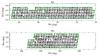 |
Fig. 1 RA–Dec distribution of galaxies in the W1 and W4 VIPERS fields for the internal catalogue version 4.0 used in this study (see text). The green lines are the survey borders that we consider in this paper. |
We structure the paper as follows: in Sect. 2 we briefly describe the VIPERS survey and the samples we derived from the data; in Sect. 3, we describe the mock galaxy catalogues used in this analysis; in Sect. 4, we describe the tests carried out to evaluate the impact of observational effects on low-density regions detection process; in Sect. 5, we describe the void-search algorithm and its application to VIPERS; in Sect. 6, we present the void-galaxy correlation function; and Sect. 7, gives our discussion of the results and conclusions.
In this paper, we adopt standard cosmological parameters matching the MultiDark simulations (Prada et al. 2012) with Ωm = 0.27, ΩΛ = 0.73 and H0 = 70 km s-1 Mpc-1.
2. The VIMOS Public Extragalactic Redshift Survey
VIPERS is an ongoing ESO programme with the goal of studying the large scale distribution of galaxies at moderate redshift (z = 0.5−1.2; Guzzo et al. 2014; Garilli et al. 2014). VIPERS is constraining the cosmological growth of structure as well as the properties of galaxies and their environments. Results include measurements of the rate of structure formation through redshift-space galaxy clustering at z = 0.8 (de la Torre et al. 2013), the dependence of galaxy clustering on luminosity and stellar mass (Marulli et al. 2013) and the galaxy stellar mass and luminosity functions (Davidzon et al. 2013; Fritz et al. 2014). The survey targets galaxies within two regions of the W1 and W4 fields of the Canada-France-Hawaii Telescope Legacy Wide (CFHTLS-Wide Survey; Cuillandre et al. 2012), shown in Fig. 1. By the end of the survey, VIPERS will cover a total sky area of 24 deg2, so that the survey area, redshift range, and relatively high sampling rate translate into similar volumes and number densities as local surveys such as 2dFGRS (Colless et al. 2003), SDSS (Strauss et al. 2002) and GAMA (Driver et al. 2011) at z = 0.3.
We carried out the observations using the VIMOS (VIsible Multi-Object Spectrograph) instrument at European Southern Observatory − Very Large Telescope (ESO-VLT; Le Fèvre et al. 2003). VIMOS is a four-channel spectrograph, with each channel corresponding to a quadrant of 7 by 8 arcmin. The position of the four quadrants leaves an unobserved cross-shaped area (of ~2 arcmin width) which is seen imprinted in the distribution of observed galaxies (see Fig. 1).
Galaxies have been targeted from the CFHTLS-Wide optical photometric catalogue with an apparent magnitude limit set to iAB ≤ 22.5. A colour selection has been used to exclude galaxies at redshift z< 0.5 (Guzzo et al. 2014). Only a fraction of the galaxies selected as potential targets may be observed because of instrumental constraints, and of these, not all are guaranteed to give a reliable redshift measurement. Nevertheless, the combination of target selection and observing strategy provides an overall sampling rate of 35%, which is extremely valuable for studying the distribution of galaxies on moderate scales.
For each galaxy, the B-band rest-frame magnitude was estimated following the spectral energy distribution (SED) fitting method described in Davidzon et al. (2013) and adopted to define volume limited samples. The choice of B-band rest-frame is natural, corresponding to the observed I-band at redshift ~0.8. We derived k and colour corrections from the best-fitting SED templates using all available photometry including near-UV, optical, and near-infrared.
2.1. Galaxy samples
The first public data release of VIPERS was made available in October 2013 and included 64% of the final dataset (Garilli et al. 2014). In this study we use the internal release version 4.0 catalogue, which increases the area of the W1 field by 30% and represents 75% of the final coverage. The angular size of the fields are 7.4 deg2 in W4 and 9.9 deg2 in W1. We select galaxies with confident spectroscopic redshifts, corresponding to zflag ≥1.5, yielding 34 965 objects in W1 and 27 258 in W4. For a detailed description of the meaning of VIPERS flag values see Guzzo et al. (2014).
We wish to perform a consistent void search across the redshift range of the survey. Therefore, we extracted two B-band rest-frame volume-limited samples from the VIPERS catalogue, one for each field (W1 and W4). As a result of galaxy evolution, the global galaxy luminosity function varies with time (Ilbert et al. 2005; Zucca et al. 2009) and the magnitude cut must therefore account for this evolution, as shown in Fig. 2. The chosen redshift range is 0.55 <z< 0.9 giving a compromise between volume explored and observed galaxy number density. The adopted magnitude limit is defined in the B-band rest-frame as  (1)where MB,lim(z) is the magnitude limit at redshift z. In the present case, the chosen value for MB,lim is − 19.8 at z = 0 (from now on, MB,lim refers to the value of the magnitude cut at z = 0).
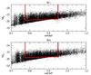 |
Fig. 2 Samples obtained form VIPERS data for the W1 and W4 fields. |
By definition the galaxy density is constant within a volume limited sample. However, in reality, this may not be exactly the case because of observational biases. Therefore we measure the mean inter-galaxy separation, within the survey mask, as a function of redshift. The mean inter-galaxy separation is defined as: 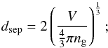 (2)where V is the survey volume, ng is the number of galaxies, and dsep/ 2 is the radius of the volume associated with each galaxy.
We measure dsep for the two fields in six redshift bins with edges at z = [ 0.55,0.65,0.70,0.75,0.80,0.85,0.90 ] (see Fig. 3). We observe that the mean separation is not constant but increases significantly in the two highest redshift bins (z = 0.8−0.85 and z = 0.85−0.9). The trend can be explained by the survey completeness that was found to decrease at fainter apparent magnitude, iAB> 20.5, due to the degradation of the redshift measurement success rate (Guzzo et al. 2014). This incompleteness of galaxies with the faintest apparent magnitudes predominantly affects the highest redshift bins in a volume-limited sample. We account for this effect when constructing the mock catalogues, as discussed in Sect. 3.
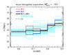 |
Fig. 3 Mean inter-galaxy separation for the W1 and W4 volume-limited samples (red and blue lines, combined value in black) and for VIPERS-like mocks (light blue lines, individual values). The green dashed line is the fit for the combined mean inter-galaxy separation of W1 and W4 fields. |
3. Mock catalogues
To test the effects of observational biases on the detection of voids, we have used mock galaxy catalogues created to have the same characteristics as the VIPERS data.
The mock catalogues are obtained from the MultiDark dark matter N-body simulation, with cosmological parameters Ωm = 0.27, Ωb = 0.0469, ΩΛ = 0.73, H0 = 70 km s-1 Mpc-1, ns = 0.95, and σ8 = 0.82 (Prada et al. 2012). The dark matter halos have been populated with galaxies using the Halo Occupation Distribution calibrated with VIPERS data. The construction of the mock catalogues can be found in de la Torre et al. (2013). The resulting mock galaxy catalogues include 26 independent realisations of the W1 survey field and 31 realisations of the W4 field. These catalogues have a redshift range of 0.4 <z< 1.3 and the same apparent magnitude limit as VIPERS (iAB< 22.5). We replicated the VIPERS target selection procedure on the mock catalogues obtaining the following samples:
-
100% mocks: containing all mock galaxies brighter than the chosen absolute magnitude limit within the survey border (indicated by the green lines in Fig. 1) but without internal gaps.
-
100% mocks real space: the same as above but using the real space positions of galaxies.
-
VIPERS-like mocks: including the survey mask and accurately reproducing the galaxy number density in the VIPERS volume limited sample that we considered.
We matched the galaxy number density in the mocks to the VIPERS data taking into account the apparent magnitude-dependent sampling rate described in Guzzo et al. (2014). The mocks well reproduce the trends observed in the real data. This is shown in Fig. 3 where the mean inter-galaxy separation measurements in the VIPERS-like mocks have been over-plotted with thin blue lines. The adopted apparent magnitude dependent sampling rates are: 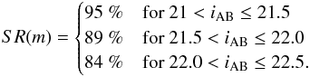
4. Tests on mock catalogues
In order to ensure that the search for voids is unhampered by the peculiar survey geometry of VIPERS, masking effects such as the gaps in each VIMOS pointing, and redshift space distortions, extensive tests were performed on the mock catalogues described in the previous section.
Galaxy counts-in-cells are a popular technique for analysing density variations in surveys (Peebles 1980) and they also provide a flexible tool for investigating the impact of complex selection effects. Furthermore it is common to use counts-in-cells to search for scarcely populated regions that are associated with voids (e.g. Hoyle & Vogeley 2002). By comparing the galaxy counts-in-cells of mocks without systematic effects to those with systematic effects added (VIPERS-like), we can evaluate the impact of observational biases (from the mask and missing quadrants) and redshift space distortions on the observed galaxy spatial distribution. We also refer the reader to Cucciati et al. (2014) for a detailed study of the impact of observational systematics on the density field estimate.
We chose the cell size to match the sizes of voids that may be found in VIPERS. As will be discussed in Sec. 5.4, the void sizes that can be reliably probed in the VIPERS data range in radius from 15 ≲ r ≲ 30 Mpc.
To compute the counts-in-cells, we randomly place a sufficient number of spherical cells inside the unmasked and undistorted mock to massively over-sample the available volume, keeping only those for which at least 80% of the volume is inside the survey borders (green lines in Fig. 1). The amount of overlap allowed between the cells and the survey boundaries is somewhat arbitrary, we find that a 20% limit provides us with enough cells to calculate robust statistics whilst not being so conservative as to dramatically reduce the effective survey volume. We then place cells at the same position in the second (masked or distorted) mock so that we can compare counts at the same position in space in the two cases.
We then identify the cells at the extremities of the histogram of the probability density function (PDF), below the 15th and above the 85th percentile for one of the samples, and then we check where these cells are placed in the distribution of the other sample. This is done for both distributions, checking where the extreme cells of the first sample are placed in the distribution of the second sample and where the extreme cells of the second sample are placed in the distribution of the first sample.
4.1. Real and redshift space
The redshift measured in a galaxy survey may be considered as a recessional velocity and is used as a proxy for distance. The measured recessional velocity is, however, the sum of a component caused by the universe’s expansion (cosmological redshift) and a proper motion component caused by gravitational interaction. This alteration of the observed positions of galaxies can thus affect both the shape and size of observed voids.
There are two types of redshift space distortion that can affect the detection of low-density regions. Firstly, linear redshift space distortions (outflow): galaxies in low-density regions are subjected to gravitational attraction from higher-density structures, and their observed position is altered such that they appear nearer to the structure than they really are (Kaiser 1986). This has the effect of further emptying the low-density regions. Secondly, non-linear redshift space distortions (the so-called fingers-of-god effect): galaxies in relaxed high-density regions (clusters) have a velocity dispersion determined by the gravitational potential well of the structure. This has the effect of stretching over densities in redshift space along the line of sight and possibly moving the observed position of some galaxies into lower-density regions (Jackson 1972).
To evaluate how redshift space distortions affect the observed distribution of galaxies we performed counts-in-cells tests on the 100% mock sample, in redshift space and real space. Examining the rank of cells in the PDF when selected in redshift space and viewed in real space (and vice versa) allows us to check if regions that we observe as being at high or low density in redshift space are truly so in real space.
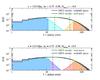 |
Fig. 4 Counts-in-cells distributions in the mock samples in redshift bin 0.75 <z< 0.9 for cells of radius r = 15 Mpc. The green line shows the distribution of counts in real space while the violet line shows the distribution in redshift space (extending slightly to higher counts). Top panel: cells are selected in redshift space. Blue and red shaded regions represent the 15% least and most populated cells in the redshift space sample, respectively. In real space the distribution of these cells are shown by the cyan and orange shaded regions. The vertical dashed line indicates the 25th and 75th percentiles of the real space distribution. Bottom panel: vice versa, cells are selected in real space and viewed in redshift space. The vertical dashed line indicates the 25th and 75th percentiles of the redshift space distribution. |
We expect redshift space distortions to have a bigger impact on smaller voids. Therefore, we show histograms for counts-in-cells for a cell radius of r = 15 Mpc, Fig. 4, in the redshift interval 0.75 <z< 0.9. The histograms show that more than 95% of cells that contribute to the 15th percentile tails of the redshift space distribution remain in the tails after transforming to real space, and, similarly, the tails selected in real space remain in the tails in redshift space. Thus, the extremities of the distribution are preserved and we can be confident that the true low-density regions in real space can be detected in redshift space.
4.2. Observational biases
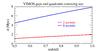 |
Fig. 5 Transverse comoving sizes of VIMOS mask cross-shaped gaps (2 arcmin) and quadrants (8 arcmin) with redshift. The sizes, in the redshift range of interest, are smaller than the dimensions of the sphere used for counts-in-cells, so we do not expect a large impact on the counts. |
How does the survey selection function, including the sampling rate and mask, affect the detection of large-scale structures? To evaluate the impact of observational biases, we compare the distribution of counts-in-cells measured in the VIPERS-like mock sample with those measured in the 100% mock sample. We do not expect an important contribution from the cross-shaped unobserved regions or from the missing quadrants, since their dimensions are smaller than the spheres we have used for the counts-in-cells (see Fig. 5). Since the comoving size of the gaps is highest in the farthest redshift bin, we expect any effect to be more relevant to small cells at higher redshift. Figure 6 presents histograms for counts-in-cells for cell radius r = 15 Mpc and redshift bin 0.75 <z< 0.9, for cells selected from the 100% and viewed in the VIPERS-like mock (and vice versa).
As for the previous tests, we see that more than 95% of the cells at the extremities of the distributions remain there after transitioning between the two samples. Also, we see that the PDF of the 100% mock sample is more skewed than that of the VIPERS-like mock, because of the reduced sampling rate. The under-sampling of the VIPERS-like mock smooths the density contrast seen in the 100% mock. The sampling rate effects dominate over the redshift-space effects discussed earlier. However, we conclude that on the scales we are interested in, masking and selection effects do not significantly introduce artificially underdense regions.
 |
Fig. 6 Counts in cells distributions in the mock samples in redshift bin 0.75 <z< 0.9 for cells of radius r = 15 Mpc. The violet line shows the distribution for the 100% samples and the green line for the VIPERS-like samples. Top panel: cells selected from the 100% sample; blue and red shaded regions represent the 15% least and most populated cells selected in the 100% samples respectively; cyan and orange shaded regions show the distribution of cells when viewed in the VIPERS-like samples. The vertical dashed line indicates the 25th and 75th percentiles of the VIPERS-like sample distribution. Bottom panel: vice versa, cells are selected from the VIPERS-like sample and viewed in the 100% sample. The vertical dashed line indicates the 25th and 75th percentiles of the 100% sample distribution. |
4.3. Sampled volume
The dimensions of the survey fields place limits on the scale of under densities that may be found. The comoving transverse sizes of the W1 and W4 fields at different redshifts are presented in Table 1. We note that the minimum dimension of the fields are a factor of ~4 times greater than the scale of the voids of interest (≳15 Mpc), over most of the redshift range.
Comoving transverse size of W1 and W4 samples.
We consider the volume of the survey fields in which we may place a spherical cell such that greater than 80% of the cell volume falls within the survey boundary. We measure this survey effective volume by randomly placing spheres of four different cell radii, between 15 and 30 Mpc, inside the survey and counting the percentage of spheres that meet the volume requirement, see Table 2.
We see that the effective volume decreases for the largest sphere sizes. Thus, we expect there to be a non-negligible selection effect on the size of the observed spheres as a function of redshift. The larger spheres whose centres are not positioned within the survey effective volume will be detected as multiple smaller spheres, further modifying the size distribution. We will discuss the impact of these effects on our measurements in the next section.
Sampled volume fraction.
5. Void detection in VIPERS
The algorithm presented in this paper is based on the detection of empty spheres, and the voids are defined as regions devoid of galaxies with absolute magnitude brighter than a specified limit (MB = −19.8 evolving with redshift). The use of spheres is a simple approximation that allows us to easily locate regions of interest. The main disadvantage is that a single sphere will not be sufficient to reconstruct the real shape of the examined empty region. Yet using spheres does not restrict our ability to detect voids of non-spherical shape. Simply, more than one sphere will be found inside the same cosmic void. Furthermore, a simple percolation analysis may be used to define a posteriori the volumes that correspond to topologically connected spheres satisfying our density cut-off (see Sect. 5.5).
5.1. Isolated and unisolated galaxies
First, the galaxies in the sample are classified as isolated or unisolated galaxies, in a similar fashion to the methods of El-Ad & Piran (1997) and Hoyle & Vogeley (2002). The idea is that, in the large-scale distribution of matter, the voids are surrounded by structures with high galaxy density (walls and filaments). The low-density regions, however, are not totally empty. They contain both void galaxies and spurious galaxies introduced to the void by redshift space distortions. Therefore, it is necessary to excise the galaxies that would cause these regions to be split into smaller volumes. Care must be taken for galaxies near the survey borders which could appear as isolated because their actual neighbouring galaxies are outside the survey limits.
We identify and remove isolated galaxies using an iterative procedure. In the algorithm, isolated galaxies are defined as galaxies far away from the survey borders with fewer than three neighbouring galaxies within a comoving sphere of radius, llim, where llim is defined from the galaxy distribution itself.
The steps are as follows.
-
1.
The distribution of the third nearest neighbour distance is computed for unisolated galaxies (initially all galaxies are classified as unisolated).
-
2.
The limit radius is calculated from this distribution. It is defined as:
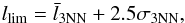 (3)where
  and σ3NN are the mean and the standard deviation of the distribution of distances to the third nearest neighbour.
 -
3.
Galaxies that do not have three neighbours within the limit are classified as isolated unless a sphere of radius l3NN, centred on the galaxy, is less than 80% inside the survey borders.
The steps converge quite rapidly and are repeated until no more isolated galaxies are found. Isolated galaxies are then removed from the sample leaving the cleaned sample. The number of isolated galaxies identified in each of the two VIPERS fields is provided in Table 3.
Detection of isolated galaxies in W1 and W4 samples.
5.2. Empty spheres
The next step of the algorithm is the search for empty spheres in the cleaned sample. A three-dimensional grid of comoving step size 1 Mpc is super-imposed on the sample. We compute the distance from each grid point to the nearest galaxy. This is the radius of the largest empty sphere centred on that point. We then calculate the volume fraction inside the survey boundaries for each sphere. Spheres with a volume fraction inside the borders lower than 80% are rejected and not included in the further analysis.
5.3. Maximal spheres
The spheres are sorted by size. The largest sphere is defined as a maximal sphere, we then check to see if the next largest sphere overlaps with this one, if it does not then it is also defined as being a maximal sphere. We continue down the list of spheres, checking for overlap with all maximal spheres already detected, until all spheres have been counted (see Fig. 7).
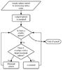 |
Fig. 7 Maximal spheres identification process. |
5.4. Statistical significance
To assess the statistical significance of maximal spheres, we compare the occurrence of these spheres to the occurrence of maximal spheres in Poisson-distributed catalogues with the same number density and mask as VIPERS. The confidence level with which we detect a maximal sphere in the galaxy distribution (over the Poisson distribution) is then given by 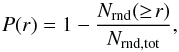 (4)where Nrnd( ≥r) is the number of maximal spheres found in the random sample with radius equal to or greater than r, and Nrnd,tot is the total number of maximal spheres in the random sample. The closer P(r) is to 1, the less likely a maximal sphere is expected to occur in a random distribution.
The number density of galaxies in the VIPERS data is not constant with redshift (see Fig. 3). Therefore, the significance limit for the radius of empty spheres will also depend on redshift. To calculate this limit we have used random catalogues with different density values. The density values correspond to the mean density values of our VIPERS fields as a function of redshift
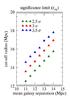 |
Fig. 8 Significant radius limit for maximal spheres as a function of the mean inter-galaxy separation for confidence levels 2, 3, and 3.5σ. |
Figure 8 shows the significance limit for maximal spheres with varying mean inter-galaxy separation for different confidence levels. As can be seen, the trend is quite linear. The relationship between the cut-off radius, corresponding to a 3σ significance for the maximal spheres, and the mean inter-galaxy separation can be described with the following fitting formula: 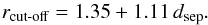 (5)Using this fit, and the trend of dsep with redshift, we find the trend of the cut-off radius with redshift. The trend for dsep is obtained by fitting the combined data from the two fields W1 and W4 where isolated galaxies have been removed (similar to what was shown in Fig. 3, where the isolated galaxies have not yet been identified), and can be described as:
  (6)Combining the two previous equations, the trend of the cut-off radius with redshift yields then the following values:
  (7)
(7)
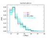 |
Fig. 9 Size distribution for maximal sphere found in W1 and W4 field samples and in VIPERS-like samples. The shaded regions correspond to the standard deviation of the measurements in the mock catalogues. |
Figure 9 shows the size distribution of the maximal spheres detected in the VIPERS survey as compared to the VIPERS-like mocks. It can be seen that the distributions obtained from the mock samples are in good agreement with measurements from the data.
Figure 10 shows the position of the maximal spheres in the two VIPERS fields projected along the RA-redshift plane. These maximal spheres correspond well to the appreciably low-density regions, as one can see by eye. We found 229 maximal spheres in the W1 field and 159 in W4. Because fields are not so extended in declination, large maximal spheres (≥25 Mpc) can only be observed in a fraction of the volume. Therefore, the number of larger spheres found is probably an underestimate.
5.5. Void percolation
The identified maximal spheres may mark the centres of individual voids or may join together to trace larger irregularly shaped voids. To identify voids traced by multiple spheres, we link together the grid centres where spheres with sizes greater than our significance limit are centred (irrespective of their being maximal or not). Groups of spheres are identified using a friends-of-friends algorithm with a linking length equal to the grid step size. The groups of sphere centres define the void regions that are connected, see Fig. 11, thus demonstrating that our method can easily be used to also define under-densities of complex shape. Void regions defined in this manner are by definition topologically distinct regions with an unisolated galaxy density lower than some threshold, δg< 1 /V(rcut − off) − 1, where V(rcut − off) is the volume of a sphere of radius rcutoff. However, the set of maximal spheres (defined in Sect. 5.3) are sufficient for the subsequent analysis presented in this paper.
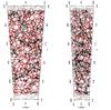 |
Fig. 10 Maximal spheres in the W1 (left) and W4 (right) samples; grey points are galaxies detected as isolated and galaxies outside the sample redshift range. The scales show comoving distance in Mpc and the corresponding redshift. |
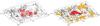 |
Fig. 11 Illustration of the region surrounding the largest maximal sphere in our catalogue (W1.0075.000), which has radius of 31 Mpc. The left-hand panel shows this sphere and the other six maximal spheres detected in this void region. The right-hand panel shows, in red, the centres of the overlapping significant spheres that make up the void, other void regions within this area of the survey are shown in orange. The black points in both panels are the unisolated galaxies, while the grey points are the isolated galaxies. |
6. Void catalogue
The catalogue of maximal spheres for both VIPERS fields is available at the CDS. The spheres are linked into larger connected voids as discussed Sect. 5.5.
The identification number of each maximal sphere is composed of: the VIPERS field to which the maximal sphere belongs (W1 or W4); a void index indicating to which void the sphere belongs (VVVV); a sphere index (SSSS) indicating the size rank of the sphere relative to other maximal spheres within the same void. The complete void ID has the form Wx.VVVV.SSSS.
For each maximal sphere of our catalogue we provide: the right ascension, declination, and redshift of the sphere’s centre; its comoving radius in Mpc; a p-value giving the detection significance with respect to a Poisson distribution.
7. Void-galaxy cross-correlation function
The void-galaxy cross-correlation function measures the probability, in excess of random, of finding a galaxy at a certain distance from the centre of a void. Cross correlations between galaxies and other astronomical objects, such as groups, clusters, and quasars, have been studied extensively (Padilla et al. 2001; Padilla & Lambas 2003; Myers et al. 2003; Yang et al. 2005; Mountrichas et al. 2009; Knobel et al. 2012). However, the study of void-galaxy cross correlations is in its infancy.
Nevertheless, the void-galaxy cross-correlation function has the potential to be a valuable statistic. It contains information that can be used to constrain models of galaxy bias (Hamaus et al. 2014). It might also be possible to use the geometrical properties of the void-galaxy cross correlation function as a standard ruler (Sutter et al. 2012a).
The void-galaxy cross correlation function contains information on the mean density profile of the voids and on the dynamics of the tracer population (Padilla et al. 2005; Paz et al. 2013). This information can be used to discriminate between different theories of gravity (Martino & Sheth 2009).
There is an on-going debate in the literature on the universality of void density profiles (Hamaus et al. 2014; Ricciardelli et al. 2014; Nadathur & Hotchkiss 2014; Nadathur et al. 2014). It is generally agreed that void density profiles can be divided broadly into two categories: compensated and uncompensated voids. Compensated voids are surrounded by an over-dense shell and may indeed be embedded in over-dense regions that are eventually going to collapse, destroying these voids. Uncompensated voids are not surrounded by an over-dense shell and represent under-dense regions that will continue to exist in the future (Sheth & van de Weygaert 2004). Our decision to include only the most significantly empty spheres in our catalogue means that our voids are relatively large. Generally they should correspond to uncompensated voids and so we should not expect to see a strong ridge in the correlation function.
The centres of the maximal spheres do not represent the centres of spherical under densities. However, in principal, there should be no preferred direction to the asymmetry of the voids in our catalogue. Therefore, stacking the maximal spheres should produce an axially symmetric density profile.
Here we search for evidence of anisotropy in the void-galaxy cross-correlation function. As previously mentioned, galaxies within voids are expected to flow towards the edge of the void under the influence of gravity. Since the redshift of a galaxy, a measure of its recessional velocity, is used as a proxy for distance, these linear outflows are expected to produce an enhancement of the void-galaxy cross-correlation function in the line of sight direction relative to the tangential direction. There should also be an apparent stretching of voids along the line of sight. However, uncertainty in defining the void centres will smooth out this effect.
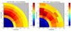 |
Fig. 12 Void-galaxy cross-correlation function, as measured in the mock catalogues (left panel) and in the VIPERS data (right panel). Measurements were made in ten radial bins and in six angular bins. The axes plotted correspond to the tangential, θ, and line of sight, π, directions. The enhancement in the line of sight direction, visible in both the mock catalogues and in the data, is evidence of redshift space distortions caused by linear outflows. |
We measured the cross-correlation function using the Davis & Peebles (1983) estimator, 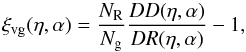 (8)where DD(η,α) and DR(η,α) are the number of void-galaxy and void-random pair counts as a function of void-galaxy separation. NR and Ng are the number of random points and the number of galaxies, respectively. The coordinates η and α are the void-galaxy radial separation (normalised to the radius of the void), η = r/Rv, and the angle between the line of sight and the line connecting the void centre with the galaxy.
The random catalogue has the same volume and angular selection function as the real data. In order to have the correct radial selection function, redshift values were randomly assigned from the redshift values of galaxies in the VIPERS-like mocks.
Other estimators, such as the Landy-Szalay estimator, are less biased than the estimator we are using, however, they require random catalogues for both sets of objects being cross-correlated. Since we cannot estimate the selection function of the voids in advance, constructing a corresponding random catalogue is not possible. Therefore, we will use the Davis and Peebles estimator.
We first measured the cross-correlation function in the mock catalogues. To maximise the total number of void-galaxy pairs we reintroduced the isolated galaxies (see Sect. 5.1) and used all the maximal spheres, including spheres close to the survey borders. This ensures that we are including all available information about the density profile of the voids.
The mean void-galaxy cross-correlation from the mock catalogues is plotted in the right-hand panel of Fig. 12. One can see that close to the origin the cross-correlation function is close to ξ ~ −1, rising to zero far away from the void centre. There is also a clear anisotropy visible. The correlation function is enhanced in the line of sight direction, peaking strongly between one and two times the radius of the maximal spheres. This is the result of linear redshift space distortions.
We then proceeded to measure the void-galaxy cross-correlation function in the VIPERS data, illustrated in the left-hand panel of Fig. 12. Similarly to the mocks, there is a clear enhancement of the correlation function in the line of sight direction.
Using the variance of the measurements of the mock catalogues we are able to calculate the χ2 between our measurement of ξvg(η,α) in the VIPERS data and in the mocks. The value quantifies the agreement between the data and mock catalogues. The computation of the χ2 requires knowing the inverse of the covariance matrix of data points. In our case, we cannot estimate it with sufficient accuracy with the mock catalogues and so we use only the variance neglecting the covariance terms. We find that the reduced χ2 = 0.49 (per degree of freedom, for the 60 η-α bins in Fig. 12), which is a very good fit. This value may be lower than expected since we have neglected the correlations between data points. This supports the validity of the concordance cosmology and the halo model used to generate the mock catalogues.
To highlight the enhancement along the line of sight we have plotted in Fig. 13 the VIPERS void-galaxy cross-correlation function as a function of radial separation for two angular bins, one close to the line of sight, α< 30°, and one close to the plane of the sky, α> 60°. One can see that, particularly in the range 1−2.5 void radii, the line of sight cross-correlation function is greater than the parallel. Furthermore, for both the α< 30° and α> 60° cases, the cross-correlation lies within the range of values measured in the mocks. This further demonstrates the good agreement between the data and the mock catalogues.
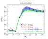 |
Fig. 13 Angle-average void-galaxy correlation function as a function of radial distance normalised to the void radius. To demonstrate the anisotropy we average over two angular wedges, along the line of sight (α< 30°, black line) and transverse to the line of sight (α> 60°, red line). The shaded regions represent the spread of values measured in the mocks. The enhancement along the line-of-sight is an indication of the redshift-space distortion produced by the outflow of galaxies from voids. |
8. Discussion and conclusions
VIMOS Public Extragalactic Redshift Survey (VIPERS; Guzzo et al. 2014) is mapping the large-scale distribution of galaxies at redshift 0.5 <z< 1.2 and provides a unique volume in which to study the distribution of voids in the galaxy distribution at moderate redshift.
The identification of voids in the galaxy distribution is challenging and it is made more difficult by observational systematics. These effects are particularly important for VIPERS, which has a complex geometry including internal gaps. The two VIPERS fields, W1 and W4, have transverse comoving dimensions of ~70 × 350 Mpc (see Table 1) and the narrow dimension further limits the volume in which we may identify large under-densities. The sampling rate is 35% to an apparent flux limit of iAB = 22.5 (Guzzo et al. 2014). In addition, the survey strategy leaves gaps in the sky coverage (see Fig. 1). Using counts-in-cell measurements on mock catalogues we investigated how observational systematics and redshift-space distortions modify the true density field. We find that on scales of r ≳ 15 Mpc the tails of the counts-in-cells PDF are well preserved such that we can truly identify the emptiest regions of the survey.
Void search methods, such as those using Voronoi tessellation (Platen et al. 2007; Neyrinck 2008; Sutter et al. 2012b), are unsuitable for this particular survey because of careful corrections required for borders and gaps. Other considerations, such as the lack of breadth in declination coverage and the limitations of the VIPERS survey strategy, make it difficult to apply void detection methods such as the water-shed method that require contiguous volumes.
In this paper, we have presented a general void-search algorithm capable of finding empty regions in a galaxy redshift survey such as VIPERS with irregular borders and internal gaps. The method is based on the identification of spheres that fit between galaxies. We show that the voids may be well characterised by keeping only the significant spheres, those that are unlikely to be found in a uniform Poisson distribution with the same number density. The significance limit for VIPERS gives voids with radii greater than ~15 Mpc. These spheres trace empty regions of arbitrary shape, as shown in Fig. 11.
The set of largest spheres that do not overlap are termed maximal spheres and we find 411 maximal spheres in the VIPERS survey with radii r ≳ 15 Mpc between 0.55 <z< 0.90. The properties of this special subset may be used to characterise the void distribution.
We present a catalogue of maximal spheres identified in VIPERS. The spheres have been associated with larger under-densities using the percolation method, thus we associate each sphere with a void ID indicating larger empty regions.
We note that the identification of the maximal spheres is affected by the survey geometry. We see that the effective volume decreases for the largest sphere sizes (Table 2). Thus, we expect there to be a noticeable selection effect. The larger spheres whose centres are not positioned within the effective volume will be detected as multiple smaller spheres, since the effective volume is larger for smaller spheres. This will affect our ability to compute some void statistics, such as the volume filling factor as a function of redshift, since the splitting of large spheres that are not found has a different impact at different redshifts. The smaller spheres could also fall below the significance limit (see Sect. 5.4), which means a loss of detected volume.
Our selection biases prevent us from drawing conclusions from the actual void size distribution, but we can directly compare the void size distribution as observed in the VIPERS data with that observed in the mocks, as both are affected by the same selection biases.
Using our catalogue of maximal spheres, we compute the void-galaxy cross-correlation function. We find an enhancement in the correlation function along the line of sight. This anisotropy is a clear signature of the velocity flows induced by the voids and matches well the signal measured in mock catalogues.
In the next phase of this work, we will fit the mean density profile of the voids and model the void-galaxy cross-correlation function (Hawken et al. in prep.). With constraints on the galaxy bias, this analysis will provide a measurement of the distortion, which may be related directly to the linear growth rate of structure, dlog δ/ dlog a. We may further characterise the distribution of voids through topological analyses. For example, the Minkowski functionals may be measured directly on the spheres complementing works on the topology of the galaxy distribution (Schimd et al., in prep.). Additionally, the isolated galaxies identified in this work can be used to study galaxy formation in low-density environments. With the detection of cosmic voids in VIPERS, we open the door to new cosmological constraints and detailed topological measurements of the distant universe.
Acknowledgments
This work is based on observations collected at the European Southern Observatory, Cerro Paranal, Chile, using the Very Large Telescope under programs 182.A-0886 and partly 070.A-9007. Also based on observations obtained with MegaPrime/MegaCam, a joint project of CFHT and CEA/DAPNIA, at the Canada-France-Hawaii Telescope (CFHT), which is operated by the National Research Council (NRC) of Canada, the Institut National des Sciences de l’Univers of the Centre National de la Recherche Scientifique (CNRS) of France, and the University of Hawaii. This work is based in part on data products produced at TERAPIX and the Canadian Astronomy Data Centre as part of the Canada-France-Hawaii Telescope Legacy Survey, a collaborative project of NRC and CNRS. The VIPERS web site is http://www.vipers.inaf.it/. We acknowledge the crucial contribution of the ESO staff for the management of service observations. In particular, we are deeply grateful to M. Hilker for his constant help and support of this program. Italian participation to VIPERS has been funded by INAF through PRIN 2008 and 2010 programs. D.M. gratefully acknowledges financial support of INAF-OABrera. L.G., A.J.H., and B.R.G. acknowledge support of the European Research Council through the Darklight ERC Advanced Research Grant (# 291521). A.P., K.M., and J.K. have been supported by the National Science Centre (grants UMO-2012/07/B/ST9/04425 and UMO-2013/09/D/ST9/04030), the Polish-Swiss Astro Project (co-financed by a grant from Switzerland, through the Swiss Contribution to the enlarged European Union), and the European Associated Laboratory Astrophysics Poland-France HECOLS. K.M. was supported by the Strategic Young Researcher Overseas Visits Program for Accelerating Brain Circulation (# R2405). O.L.F. acknowledges support of the European Research Council through the EARLY ERC Advanced Research Grant (# 268107). G.D.L. acknowledges financial support from the European Research Council under the European Community’s Seventh Framework Programme (FP7/2007-2013)/ERC grant agreement # 202781. W.J.P. and R.T. acknowledge financial support from the European Research Council under the European Community’s Seventh Framework Programme (FP7/2007-2013)/ERC grant agreement # 202686. W.J.P. is also grateful for support from the UK Science and Technology Facilities Council through the grant ST/I001204/1. E.B., F.M. and L.M. acknowledge the support from grants ASI-INAF I/023/12/0 and PRIN MIUR 2010-2011. L.M. also acknowledges financial support from PRIN INAF 2012. Y.M. acknowledges support from CNRS/INSU (Institut National des Sciences de l’Univers) and the Programme National Galaxies et Cosmologie (PNCG). C.M. is grateful for support from specific project funding of the Institut Universitaire de France and the LABEX OCEVU.
References
- Alpaslan, M., Robotham, A. S. G., Obreschkow, D., et al. 2014, MNRAS, 440, L106 [Google Scholar]
- Benson, A. J., Hoyle, F., Torres, F., & Vogeley, M. S. 2003, MNRAS, 340, 160 [NASA ADS] [CrossRef] [Google Scholar]
- Betancort-Rijo, J., Patiri, S. G., Prada, F., & Romano, A. E. 2009, MNRAS, 400, 1835 [NASA ADS] [CrossRef] [Google Scholar]
- Biswas, R., Alizadeh, E., & Wandelt, B. D. 2010, Phys. Rev. D, 82, 023002 [NASA ADS] [CrossRef] [Google Scholar]
- Bos, E. G. P., van de Weygaert, R., Dolag, K., & Pettorino, V. 2012, MNRAS, 426, 440 [NASA ADS] [CrossRef] [Google Scholar]
- Ceccarelli, L., Paz, D., Lares, M., Padilla, N., & Lambas, D. G. 2013, MNRAS, 434, 1435 [NASA ADS] [CrossRef] [Google Scholar]
- Chincarini, G. 1978, Nature, 272, 515 [NASA ADS] [CrossRef] [Google Scholar]
- Chincarini, G., & Rood, H. J. 1976, ApJ, 206, 30 [NASA ADS] [CrossRef] [Google Scholar]
- Chincarini, G., & Rood, H. J. 1979, ApJ, 230, 648 [NASA ADS] [CrossRef] [Google Scholar]
- Clampitt, J., & Jain, B. 2014 [arXiv:1404.1834] [Google Scholar]
- Clampitt, J., Cai, Y.-C., & Li, B. 2013, MNRAS, 431, 749 [NASA ADS] [CrossRef] [Google Scholar]
- Colless, M., Peterson, B. A., Jackson, C., et al. 2003 [arXiv:astro-ph/0306581] [Google Scholar]
- Colberg, J. M., Sheth, R. K., Diaferio, A., Gao, L., & Yoshida, N. 2005, MNRAS, 360, 216 [NASA ADS] [CrossRef] [Google Scholar]
- Cucciati, O., Granett, B. R., Branchini, E., et al. 2014, A&A, 565, A67 [NASA ADS] [CrossRef] [EDP Sciences] [Google Scholar]
- Cuillandre, J.-C. J., Withington, K., Hudelot, P., et al. 2012, in SPIE Conf. Ser., 8448 [Google Scholar]
- Davidzon, I., Bolzonella, M., Coupon, J., et al. 2013, A&A, 558, A23 [NASA ADS] [CrossRef] [EDP Sciences] [Google Scholar]
- Davis, M., & Peebles, P. J. E. 1983, ApJ, 267, 465 [NASA ADS] [CrossRef] [Google Scholar]
- Davis, M., Huchra, J., Latham, D. W., & Tonry, J. 1982, ApJ, 253, 423 [NASA ADS] [CrossRef] [Google Scholar]
- de la Torre, S., Guzzo, L., Peacock, J. A., et al. 2013, A&A, 557, A54 [NASA ADS] [CrossRef] [EDP Sciences] [Google Scholar]
- de Lapparent, V., Geller, M. J., & Huchra, J. P. 1986, ApJ, 302, L1 [NASA ADS] [CrossRef] [Google Scholar]
- Dekel, A., & Rees, M. J. 1994, ApJ, 422, L1 [NASA ADS] [CrossRef] [Google Scholar]
- Driver, S. P., Hill, D. T., Kelvin, L. S., et al. 2011, MNRAS, 413, 971 [NASA ADS] [CrossRef] [Google Scholar]
- El-Ad, H., & Piran, T. 1997, ApJ, 491, 421 [NASA ADS] [CrossRef] [Google Scholar]
- Fritz, A., Scodeggio, M., Ilbert, O., et al. 2014, A&A, 563, A92 [NASA ADS] [CrossRef] [EDP Sciences] [Google Scholar]
- Garilli, B., Guzzo, L., Scodeggio, M., et al. 2014, A&A, 562, A23 [NASA ADS] [CrossRef] [EDP Sciences] [Google Scholar]
- Gregory, S. A., & Thompson, L. A. 1978, ApJ, 222, 784 [NASA ADS] [CrossRef] [Google Scholar]
- Guzzo, L., Scodeggio, M., Garilli, B., et al. 2014, A&A, 566, A108 [NASA ADS] [CrossRef] [EDP Sciences] [Google Scholar]
- Hamaus, N., Wandelt, B. D., Sutter, P. M., Lavaux, G., & Warren, M. S. 2014, Phys. Rev. Lett., 112, 041304 [NASA ADS] [CrossRef] [Google Scholar]
- Hernández-Monteagudo, C., & Smith, R. E. 2013, MNRAS, 435, 1094 [NASA ADS] [CrossRef] [Google Scholar]
- Hoyle, F., & Vogeley, M. S. 2002, ApJ, 566, 641 [NASA ADS] [CrossRef] [Google Scholar]
- Icke, V. 1984, MNRAS, 206, 1P [NASA ADS] [CrossRef] [Google Scholar]
- Ilbert, O., Tresse, L., Zucca, E., et al. 2005, A&A, 439, 863 [NASA ADS] [CrossRef] [EDP Sciences] [Google Scholar]
- Ilić, S., Langer, M., & Douspis, M. 2013, A&A, 556, A51 [NASA ADS] [CrossRef] [EDP Sciences] [Google Scholar]
- Jõeveer, M., Einasto, J., & Tago, E. 1978, MNRAS, 185, 357 [NASA ADS] [CrossRef] [Google Scholar]
- Jackson, J. C. 1972, MNRAS, 156, 1P [Google Scholar]
- Kaiser, N. 1986, MNRAS, 222, 323 [NASA ADS] [CrossRef] [Google Scholar]
- Knobel, C., Lilly, S. J., Carollo, C. M., et al. 2012, ApJ, 755, 48 [NASA ADS] [CrossRef] [Google Scholar]
- Lavaux, G., & Wandelt, B. D. 2010, MNRAS, 403, 1392 [NASA ADS] [CrossRef] [Google Scholar]
- Le Fèvre, O., Saisse, M., Mancini, D., et al. 2003, in SPIE Conf. Ser. 4841, eds. M. Iye, & A. F. M. Moorwood, 1670 [Google Scholar]
- Martino, M. C., & Sheth, R. K. 2009 [arXiv:0911.1829] [Google Scholar]
- Marulli, F., Bolzonella, M., Branchini, E., et al. 2013, A&A, 557, A17 [NASA ADS] [CrossRef] [EDP Sciences] [Google Scholar]
- Mountrichas, G., Sawangwit, U., Shanks, T., et al. 2009, MNRAS, 394, 2050 [NASA ADS] [CrossRef] [Google Scholar]
- Myers, A. D., Outram, P. J., Shanks, T., et al. 2003, MNRAS, 342, 467 [NASA ADS] [CrossRef] [Google Scholar]
- Nadathur, S., & Hotchkiss, S. 2014, MNRAS, 440, 1248 [NASA ADS] [CrossRef] [Google Scholar]
- Nadathur, S., Hotchkiss, S., Diego, J. M., et al. 2014, MNRAS, submitted [arXiv:1407.1295] [Google Scholar]
- Neyrinck, M. C. 2008, MNRAS, 386, 2101 [NASA ADS] [CrossRef] [Google Scholar]
- Padilla, N. D., & Lambas, D. G. 2003, MNRAS, 342, 532 [NASA ADS] [CrossRef] [Google Scholar]
- Padilla, N. D., Merchán, M. E., Valotto, C. A., Lambas, D. G., & Maia, M. A. G. 2001, ApJ, 554, 873 [NASA ADS] [CrossRef] [Google Scholar]
- Padilla, N. D., Ceccarelli, L., & Lambas, D. G. 2005, MNRAS, 363, 977 [NASA ADS] [CrossRef] [Google Scholar]
- Park, D., & Lee, J. 2007, Phys. Rev. Lett., 98, 081301 [NASA ADS] [CrossRef] [Google Scholar]
- Paz, D., Lares, M., Ceccarelli, L., Padilla, N., & Lambas, D. G. 2013, MNRAS, 436, 3480 [NASA ADS] [CrossRef] [Google Scholar]
- Peebles, P. J. E. 1980, The large-scale structure of the universe (Princeton University Press) [Google Scholar]
- Platen, E., van de Weygaert, R., & Jones, B. J. T. 2007, MNRAS, 380, 551 [NASA ADS] [CrossRef] [Google Scholar]
- Prada, F., Klypin, A. A., Cuesta, A. J., Betancort-Rijo, J. E., & Primack, J. 2012, MNRAS, 423, 3018 [NASA ADS] [CrossRef] [Google Scholar]
- Regos, E., & Geller, M. J. 1991, ApJ, 377, 14 [NASA ADS] [CrossRef] [Google Scholar]
- Ricciardelli, E., Quilis, V., & Varela, J. 2014, MNRAS, 440, 601 [NASA ADS] [CrossRef] [Google Scholar]
- Rood, H. J. 1988a, PASP, 100, 1071 [NASA ADS] [CrossRef] [Google Scholar]
- Rood, H. J. 1988b, ARA&A, 26, 245 [NASA ADS] [CrossRef] [Google Scholar]
- Ryden, B. S. 1995, ApJ, 452, 25 [NASA ADS] [CrossRef] [Google Scholar]
- Ryden, B. S., & Melott, A. L. 1996, ApJ, 470, 160 [NASA ADS] [CrossRef] [Google Scholar]
- Sheth, R. K., & van de Weygaert, R. 2004, MNRAS, 350, 517 [NASA ADS] [CrossRef] [Google Scholar]
- Spolyar, D., Sahlén, M., & Silk, J. 2013, Phys. Rev. Lett., 111, 241103 [NASA ADS] [CrossRef] [Google Scholar]
- Strauss, M. A., Weinberg, D. H., Lupton, R. H., et al. 2002, AJ, 124, 1810 [NASA ADS] [CrossRef] [Google Scholar]
- Sutter, P. M., Lavaux, G., Wandelt, B. D., & Weinberg, D. H. 2012a, ApJ, 761, 187 [NASA ADS] [CrossRef] [Google Scholar]
- Sutter, P. M., Lavaux, G., Wandelt, B. D., & Weinberg, D. H. 2012b, ApJ, 761, 44 [NASA ADS] [CrossRef] [Google Scholar]
- Tarenghi, M., Tifft, W. G., Chincarini, G., et al. 1978, in Large Scale Structures in the Universe, eds. M. S. Longair, & J. Einasto, IAU Symp., 79, 263 [Google Scholar]
- Tifft, W. G., & Gregory, S. A. 1976, ApJ, 205, 696 [NASA ADS] [CrossRef] [Google Scholar]
- Tully, R. B., & Fisher, J. R. 1978, in Large Scale Structures in the Universe, eds. M. S. Longair, & J. Einasto, IAU Symp., 79, 214 [Google Scholar]
- White, S. D. M. 1979, MNRAS, 186, 145 [NASA ADS] [CrossRef] [Google Scholar]
- Yang, X., Mo, H. J., van den Bosch, F. C., et al. 2005, MNRAS, 362, 711 [NASA ADS] [CrossRef] [Google Scholar]
- Zucca, E., Bardelli, S., Bolzonella, M., et al. 2009, A&A, 508, 1217 [NASA ADS] [CrossRef] [EDP Sciences] [Google Scholar]
All Tables
All Figures
|
Fig. 1 RA–Dec distribution of galaxies in the W1 and W4 VIPERS fields for the internal catalogue version 4.0 used in this study (see text). The green lines are the survey borders that we consider in this paper. |
| In the text | |
|
Fig. 2 Samples obtained form VIPERS data for the W1 and W4 fields. |
| In the text | |
|
Fig. 3 Mean inter-galaxy separation for the W1 and W4 volume-limited samples (red and blue lines, combined value in black) and for VIPERS-like mocks (light blue lines, individual values). The green dashed line is the fit for the combined mean inter-galaxy separation of W1 and W4 fields. |
| In the text | |
|
Fig. 4 Counts-in-cells distributions in the mock samples in redshift bin 0.75 <z< 0.9 for cells of radius r = 15 Mpc. The green line shows the distribution of counts in real space while the violet line shows the distribution in redshift space (extending slightly to higher counts). Top panel: cells are selected in redshift space. Blue and red shaded regions represent the 15% least and most populated cells in the redshift space sample, respectively. In real space the distribution of these cells are shown by the cyan and orange shaded regions. The vertical dashed line indicates the 25th and 75th percentiles of the real space distribution. Bottom panel: vice versa, cells are selected in real space and viewed in redshift space. The vertical dashed line indicates the 25th and 75th percentiles of the redshift space distribution. |
| In the text | |
|
Fig. 5 Transverse comoving sizes of VIMOS mask cross-shaped gaps (2 arcmin) and quadrants (8 arcmin) with redshift. The sizes, in the redshift range of interest, are smaller than the dimensions of the sphere used for counts-in-cells, so we do not expect a large impact on the counts. |
| In the text | |
|
Fig. 6 Counts in cells distributions in the mock samples in redshift bin 0.75 <z< 0.9 for cells of radius r = 15 Mpc. The violet line shows the distribution for the 100% samples and the green line for the VIPERS-like samples. Top panel: cells selected from the 100% sample; blue and red shaded regions represent the 15% least and most populated cells selected in the 100% samples respectively; cyan and orange shaded regions show the distribution of cells when viewed in the VIPERS-like samples. The vertical dashed line indicates the 25th and 75th percentiles of the VIPERS-like sample distribution. Bottom panel: vice versa, cells are selected from the VIPERS-like sample and viewed in the 100% sample. The vertical dashed line indicates the 25th and 75th percentiles of the 100% sample distribution. |
| In the text | |
|
Fig. 7 Maximal spheres identification process. |
| In the text | |
|
Fig. 8 Significant radius limit for maximal spheres as a function of the mean inter-galaxy separation for confidence levels 2, 3, and 3.5σ. |
| In the text | |
|
Fig. 9 Size distribution for maximal sphere found in W1 and W4 field samples and in VIPERS-like samples. The shaded regions correspond to the standard deviation of the measurements in the mock catalogues. |
| In the text | |
|
Fig. 10 Maximal spheres in the W1 (left) and W4 (right) samples; grey points are galaxies detected as isolated and galaxies outside the sample redshift range. The scales show comoving distance in Mpc and the corresponding redshift. |
| In the text | |
|
Fig. 11 Illustration of the region surrounding the largest maximal sphere in our catalogue (W1.0075.000), which has radius of 31 Mpc. The left-hand panel shows this sphere and the other six maximal spheres detected in this void region. The right-hand panel shows, in red, the centres of the overlapping significant spheres that make up the void, other void regions within this area of the survey are shown in orange. The black points in both panels are the unisolated galaxies, while the grey points are the isolated galaxies. |
| In the text | |
|
Fig. 12 Void-galaxy cross-correlation function, as measured in the mock catalogues (left panel) and in the VIPERS data (right panel). Measurements were made in ten radial bins and in six angular bins. The axes plotted correspond to the tangential, θ, and line of sight, π, directions. The enhancement in the line of sight direction, visible in both the mock catalogues and in the data, is evidence of redshift space distortions caused by linear outflows. |
| In the text | |
|
Fig. 13 Angle-average void-galaxy correlation function as a function of radial distance normalised to the void radius. To demonstrate the anisotropy we average over two angular wedges, along the line of sight (α< 30°, black line) and transverse to the line of sight (α> 60°, red line). The shaded regions represent the spread of values measured in the mocks. The enhancement along the line-of-sight is an indication of the redshift-space distortion produced by the outflow of galaxies from voids. |
| In the text | |
Current usage metrics show cumulative count of Article Views (full-text article views including HTML views, PDF and ePub downloads, according to the available data) and Abstracts Views on Vision4Press platform.
Data correspond to usage on the plateform after 2015. The current usage metrics is available 48-96 hours after online publication and is updated daily on week days.
Initial download of the metrics may take a while.