| Issue |
A&A
Volume 570, October 2014
|
|
|---|---|---|
| Article Number | A98 | |
| Number of page(s) | 9 | |
| Section | Cosmology (including clusters of galaxies) | |
| DOI | https://doi.org/10.1051/0004-6361/201423958 | |
| Published online | 30 October 2014 | |
Cross-correlation of cosmic far-infrared background anisotropies with large scale structures⋆
1
Institut d’Astrophysique Spatiale (IAS), Bâtiment 121, Université Paris-Sud
11 and CNRS (UMR 8617),
91405
Orsay,
France
e-mail:
This email address is being protected from spambots. You need JavaScript enabled to view it.
2
Jet Propulsion Laboratory, California Institute of
Technology, 4800 Oak Grove
Drive, Pasadena,
California,
USA
3
California Institute of Technology, Pasadena, California, USA
4
Department of Physics, University of California Berkeley, CA 94720,
USA
5
Lawrence Berkeley National Laboratory,
1 Cyclotron Rd, Berkeley, CA
94720,
USA
Received: 7 April 2014
Accepted: 25 August 2014
Abstract
We measure the cross-power spectra between luminous red galaxies (LRGs) from the Sloan Digital Sky Survey (SDSS)-III data release 8 (DR8) and cosmic infrared background (CIB) anisotropies from Planck and data from the Improved Reprocessing (IRIS) of the Infrared Astronomical Satellite (IRAS) at 353, 545, 857, and 3000 GHz, corresponding to 850, 550, 350 and 100 μm, respectively, in the multipole range 100 < l < 1000. Using approximately 6.5 × 10⁵ photometrically determined LRGs in 7760 deg2 of the northern hemisphere in the redshift range 0.45 < z < 0.65, we model the far-infrared background (FIRB) anisotropies with an extended version of the halo model. With these methods, we confirm the basic picture obtained from recent analyses of FIRB anisotropies with Herschel and Planck, that the most efficient halo mass at hosting star forming galaxies is log (Meff/M⊙) = 12.84 ± 0.15. We estimate the percentage of FIRB anisotropies correlated with LRGs as approximately 11.8%, 3.9%, 1.8%, and 1.0% of the total at 3000, 857, 545, and 353 GHz, respectively. At redshift z ~ 0.55, the bias of FIRB galaxies with respect to the dark matter density field has the value bFIRB ~ 1.45, and the mean dust temperature of FIRB galaxies is Td = 26 K. Finally, we discuss the impact of present and upcoming cross-correlations with far-infrared background anisotropies on the determination of the global star formation history and the link between galaxies and dark matter.
Key words: cosmic background radiation / infrared: diffuse background / galaxies: evolution / large-scale structure of Universe / galaxies: statistics
Based on observations obtained with Planck (http://www.esa.int/Planck), an ESA science mission with instruments and contributions directly funded by ESA Member States, NASA, and Canada.
© ESO, 2014
1. Introduction
The cosmic infrared background (CIB), detected with both the Far InfraRed Absolute Spectrophotometer (FIRAS, Puget et al. 1996; Fixsen et al. 1998; Lagache et al. 1999) and the Diffuse Infrared Background Experiment (DIRBE, Hauser et al. 1998; Lagache et al. 2000), accounts for approximately half of the total energy radiated by structure formation processes throughout cosmic history since the end of the matter-radiation decoupling epoch (Dole et al. 2006). Early attempts at measuring CIB fluctuations at near-infrared wavelengths have been performed from degree to sub-arcminute scales using data from COBE/DIRBE (Kashlinsky & Odenwald 2000), IRTS/NIRS (Matsumoto et al. 2005), 2MASS (Kashlinsky et al. 2002), and Spitzer-IRAC (Kashlinsky et al. 2005). On the other end, fluctuations in the cosmic far-infrared background (FIRB), composed of thermal emission from warm dust enshrouding star-forming regions in galaxies, have been reported using the ISOPHOT instrument aboard the Infrared Space Observatory (Matsuhara et al. 2000; Lagache & Puget 2000), the Spitzer Space Telescope (Lagache et al. 2007), the BLAST balloon experiment (Viero et al. 2009), and the Herschel Space Observatory (Amblard et al. 2011). In the same period, different cosmic microwave background (CMB) experiments extended these detections to longer wavelengths (Hall et al. 2010; Dunkley et al. 2011; Reichardt et al. 2012). The Planck early results paper Planck Collaboration XVIII 2011 measured angular power spectra of CIB anisotropies from arc-minute to degree scales at 217, 353, 545, and 857 GHz and the recent paper Planck Collaboration XXX 2014 represents its extension and improvement in terms of analysis and interpretation, establishing Planck as a powerful probe of the FIRB clustering.
The far-infrared component of the CIB radiation (or far-infrared background, FIRB) is primarily due to dusty, star-forming galaxies (DSFGs). The dust absorbs the optical and ultraviolet stellar radiation and re-emits in the infrared and submillimetre (submm) wavelengths. The rest frame spectral energy distribution (SED) of DSFGs peaks near 100 μm, and it moves into the FIR/submm regime as objects at increasing redshifts are observed. Thus, a complete understanding of the star formation history (SFH) in the Universe must involve accurate observations in the FIR/submm wavelength range.
FIRB anisotropies are a powerful probe of the global SFH. However, because the signal is integrated over all redshifts, it prevents a detailed investigation of the temporal evolution of DSFGs over cosmic time. Cross-correlation studies are a powerful expedient to remedy this fact. Because DSFGs trace the underlying dark matter field, a certain degree of correlation between the CIB and any other tracer of the dark matter distribution is expected, provided that some overlap in redshifts exists between the tracers. A useful property of such cross-correlation studies is that the measurement can be used to isolate and analyze a small redshift range in one signal (e.g., the CIB) if the other population is limited in redshift (e.g., the LRGs). In addition, the measurement is not prone to systematics that are not correlated between the two datasets, giving thus a strong signal even if each dataset is contaminated by other physical effects. As shown in Planck Collaboration XXX (2014) for example, foreground Galactic dust severely limits CIB measurements at the high frequency channels (ν ≥ 545 GHz) while CMB anisotropies contaminate the CIB signal at frequencies ν ≤ 353 GHz; possible approaches to dealing with these foregrounds include their inclusion in the likelihood analysis (e.g., as a power law) or their removal using a tracer of dust and possibly selecting very clean regions of the sky. In any event, the presence of foreground and background contamination greatly complicates the analysis of CIB data. This limitation disappears when cross-correlating CIB maps with catalogs of dark matter tracers not directly correlated with Galactic dust or CMB (e.g., Planck Collaboration XVIII 2014); in this case, the presence of uncorrelated contaminants only appears in the computation of the uncertainties associated with the measurement.
In this paper, we perform a measurement of the cross-correlation between FIRB maps from Planck and maps from the Improved Reprocessing (IRIS) of the Infrared Astronomical Satellite (IRAS) with a galaxy map of luminous red galaxies (LRGs) from SDSS-III data release 8 (DR8). By fixing both the LRGs redshift distribution and their bias with respect to the dark matter field, we will be able to constrain the most efficient dark matter halo mass at hosting star formation in DSFGs, with their SED. The existence of such a characteristic halo mass has been predicted both analytically and with numerical simulations, and it constitutes a critical component that triggers the growth and assembly of stars in galaxies. After comparing our results with recent analyses in the literature, we will outline the role of upcoming cross-correlation studies with many tracers of the dark matter field in multiple redshift bins, in constraining the redshift evolution of the link between dark matter and star formation, thus bringing new insight into the cosmic SFH. A measurement of the cross-correlation between FIRB sources and other tracers of the dark matter field at high redshift can be extremely important in constraining the early star formation history of the Universe and the clustering properties of high-redshift objects. In this regard, it is important to keep in mind that a good knowledge of the redshift distribution of the sources to be cross-correlated with the FIRB is mandatory in order to constrain both the FIRB emissivity and the bias of both tracers. The quasars catalog from the Wide-field Infrared Survey Explorer (WISE, Wright et al. 2010), whose redshift distribution can be inferred using the method developed in, e.g., Ménard et al. (2013), and the spectroscopic quasars from the Baryon Oscillation Spectroscopic Survey (BOSS, Pâris et al. 2014) will certainly be important for such studies. However, our very thorough attempt at computing their cross-power spectrum with the FIRB maps has shown the existence of possible systematics that have not been well understood. In particular, when cross-correlating with the spectroscopic BOSS quasar catalog, we find a strong anti-correlation at large angular scales whose origin, among many possibilities, has not been clearly isolated. On the other hand, the difficulty in selecting objects in the WISE dataset (beyond the approximate method based on color cuts explained in Wright et al. 2010), does not allow us to clearly interpret the results of the cross-correlation in the context of the halo model. We thus decided not to include these datasets in the present analysis and to defer this kind of study to a future publication.
Throughout this paper, we adopt the standard flat ΛCDM cosmological model as our fiducial background cosmology, with parameter values derived from the best-fit model of the CMB power spectrum measured by Planck (Planck Collaboration XVI 2014): { Ωm,ΩΛ,Ωbh2,σ8,h,ns } = { 0.3175,0.6825,0.022068,0.8344,0.6711,0.9624 }. We also define halos as matter overdense regions with a mean density equal to 200 times the mean density of the Universe, and we assume a Navarro-Frenck-White (NFW) profile (Navarro et al. 1997) with a concentration parameter as in Cooray & Sheth (2002). The fitting function of Tinker et al. (2008) is used for the halo-mass function while sub-halo mass function and halo bias are taken as in Tinker et al. (2010).
2. Data
2.1. CMASS catalog
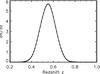 |
Fig. 1 Normalized SDSS-III DR8 LRG redshift distribution, peaked at |

The galaxy sample used in the cross-correlation analysis consists of LRGs selected from the publicly available SDSS-III DR8 catalog1 (Eisenstein et al. 2011; Ross et al. 2011; Ho et al. 2012; de Putter et al. 2012), with photometric redshift in the range 0.45 < zphot < 0.65, and centered around  (see Fig. 1). We considered the same color and magnitude cuts as the SDSS-III “CMASS” (constant mass) sample from BOSS (White et al. 2011; Ho et al. 2012) and, to create a galaxy map from the catalog, we used the HEALPix2 pixelization scheme of the sphere (Górski et al. 2005) at resolution Nside =1024; objects are weighted with their probability of being a galaxy and pixelized as number overdensities δi with respect to the mean number of galaxies
  in each pixel, as:
 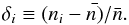 (1)Complex survey geometries due to partial sky coverage and masked regions can cause numerical issues and power leakage from large to small scales when performing power spectra computations, especially when using estimators in harmonic space. Because the southern hemisphere footprint has a complicated geometry and it contributes few additional galaxies, to be as conservative as possible, we discard it and only use data in the northern hemisphere. This choice reduces the total area available of approximately 1300 deg2, leaving 7760 deg2 with approximately 650 000 galaxies, but ensures stability of results, as we will show below, where we confront error bars computed analytically with those estimated from Monte Carlo simulations. An accurate analysis of potential systematics affecting our dataset, stressing the contribution of seeing effects, sky brightness, and stellar contamination, has been performed in Ross et al. (2011) and Ho et al. (2012), and we will shape our galaxy mask according to their prescriptions to reduce these effects.
As shown in Fig. 2, the computation of the LRG auto-power spectrum from these data is compatible with a non linear prescription for the dark matter power spectrum (we used the Halofit routine (Smith et al. 2003) in CAMB3), together with a scale and redshift independent galaxy bias parameter bLRG = 2.1 ± 0.02 in agreement with Ross et al. (2011), and with a galaxy redshift distribution centered in and with spread σ = 0.07: 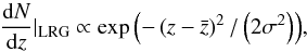 (2)as shown in Fig. 1.
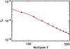 |
Fig. 2 Angular auto-power spectrum measured in the SDSS-III DR8 LRG survey. |
In the rest of our analysis, we use Eq. (2) to compute the LRG redshift distribution and we fix the LRG bias to the value bLRG = 2.1.
2.2. Planck and IRIS maps
We use intensity maps at 353, 545, and 857 GHz from the public data release of the first 15.5 months of Planck operations (Planck Collaboration I 2014), with a far-infrared map at 3000 GHz from IRAS (IRIS, Miville-Deschênes et al. 2002; Miville-Deschênes & Lagache 2005). We do not use the lower frequency Planck channels in our analysis, as they contain a large contribution from primary CMB anisotropies and, for the redshift distribution of the galaxy sample considered here, most of the cross-correlation signal comes from the higher frequency maps. Finally, the large number of point sources to be masked in the IRAS 3000 GHz map creates mask irregularities that prevent a stable computation of the cross-power spectrum for multipoles ℓ> 500; we thus consider only measurements at multipoles ℓ < 500 at 3000 GHz.
We refer the reader to Planck Collaboration VI (2014); Planck Collaboration VII (2014); Planck Collaboration VIII (2014) for details related to the mapmaking pipeline, beam description and, in general, to the data processing for HFI data. We used two masks to exclude regions with diffuse Galactic emission and extragalactic point sources. The first mask accounts for diffuse Galactic emission as observed in the Planck data and leaves approximately 60% of the sky unmasked4. The second mask has been created using the Planck Catalogue of Compact Sources (PCCS, Planck Collaboration XXVIII 2014) to identify point sources with signal-to-noise ratio greater or equal to five in the maps, and masking out a circular area of 3σ radius around each source (where σ = FWHM/ 2.35). The point sources to be removed have flux densities above a given threshold, as explained in Planck Collaboration XXX (2014). At 3000 GHz, we used a more aggressive mask, which leaves 20% of the sky unmasked and covers dust contaminated regions at high latitudes more efficiently. The final footprint used in our cross-correlation analysis, which is simply the product of the LRG mask with each of the four FIRB masks, has been smoothed with a Gaussian beam with full width at half maximum of ten arcminutes, to reduce possible power leakage; the mask used for the 857 GHz channel is shown in Fig. 3.
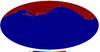 |
Fig. 3 Apodized mask used to cross-correlate the DR8 LRG map with the Planck temperature map at 857 GHz; the sky fraction unmasked is approximately fsky = 0.185. |
3. Cross-correlation measurement and analysis
We work in harmonic space, using anafast from the HEALPix package to cross-correlate temperature and density maps and applying the pseudo-Cℓ technique described in Hivon et al. (2002) to deconvolve both mask and beam effects from the cross-power spectrum.
A generic scalar field  defined over the full-sky can be expressed in terms of spherical harmonics
  as:
as:  (3)where al,m denotes the spherical harmonic coefficients:
  (4)and, for isotropic temperature and galaxy fields, it is possible to write their cross-power spectrum
  as:
as:  (5)where δK denotes the Kronecker delta function.
Because of contamination or partial sky coverage, we often have access only to a given fraction of the sky. For a generic partial sky map, the resulting power spectrum (called pseudo power spectrum  ) is different from the full-sky power spectrum Cl, but their ensemble averages are related by:
  (6)The coupling matrix Ml,l′, computed with the mixing matrix formalism introduced in Hivon et al. (2002), encompasses the combined effects of partial sky coverage, beam, and pixel respectively, and it is obtained by:
  (7)where we introduced the Wigner 3-j symbol (or Clebsch-Gordan coefficient)
  , and Bl is a window function describing the combined smoothing effect due to the beam and finite pixel size.
3.1. Error bars computation
Our measurements are obtained as binned power spectra with a binning Δℓ = 100, and we use a Monte Carlo approach to compute the uncertainty associated with each bin. In particular, we simulate N = 500 pairs of FIRB temperature and LRG density maps, correlated as expected theoretically, adding the expected Poisson noise to both maps, in addition to an instrumental noise and a Galactic dust “noise” term to the FIRB frequency maps. More specifically, our pipeline for the computation of error bars, also described in, e.g., Giannantonio et al. (2008), works as follows:
-
A simulated FIRB frequency map is created (using the programsynfast from the HEALPix package) as the sum of a clusteringterm plus three noise contributions due to shot noise, Galacticdust contamination, and instrument noise. The total powerspectrum to be used as input in synfast can be written as follows:
 (8)Using the Limber approximation (Limber 1953), valid on all scales considered in our analysis, the clustering term for each frequency ν is simply computed as:
  (9)here χ(z) is the comoving angular diameter distance to redshift z, Pdm(k,z) is the dark matter power spectrum, while bFIRB(k,z) and
  denote the bias of the FIRB sources and the redshift distribution of their emissivity, respectively. Values for the shot-noise power spectrum
  are obtained from Table 9 of Planck Collaboration XXX (2014). For the dust power spectrum we use a template taken as a power law
  , where the amplitude K and the slope α are computed by fitting the measured dust-power spectrum from our CIB maps. Finally, the Planck instrument noise power spectrum
  is estimated from the jack-knife difference maps, using the first and second halves of each pointing period (see also Planck Collaboration XXX 2014). We refer to Miville-Deschênes et al. (2002) for the IRAS noise power spectrum computation.
 -
A galaxy map is also created as a sum of a clustering plus a shot-noise term:
 (10)In the Limber approximation, the clustering term can be expressed as:
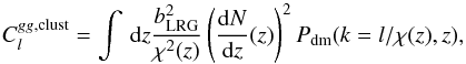 (11)and the shot noise power spectrum
  is directly estimated from the measured number of galaxies per pixel. The galaxy map must be correlated with the FIRB map. In general, two correlated galaxy-temperature maps are described by three power spectra,
  ,
,  , and
, and  , where the last term is given by:
 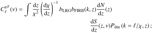 (12)It is easy to correlate a galaxy map with a given FIRB map created with synfast. First, we build a FIRB map with a power spectrum
  ; then, we make a second map with the same synfast seed used for the clustering term
  and with power spectrum
  and we add this second map to a third map made with a new seed and with power spectrum
  . These two maps will have amplitudes:
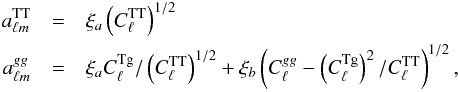 (13)where ξ denotes a random amplitude, which is a complex number with zero mean and unit variance (⟨ ξξ∗ ⟩ = 1 and ⟨ ξ ⟩ = 0). These amplitudes yield:
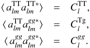 (14)The obtained maps are then masked with the same mask as that we used to analyze the real data and the cross-power spectrum is then computed using the pseudo-power spectrum technique as in Hivon et al. (2002). The set of realizations of the cross-power spectrum provides the uncertainty in our estimate. The covariance matrix of the binned power spectrum Cb is:
 (15)with ⟨·⟩ standing for Monte Carlo averaging. The error bars on each binned Cb is:
 (16)The error bars computed from simulations have been also compared with an analytic estimate of the uncertainty, given by:
 ![Mathematical equation: \begin{equation} \label{eq:ana_error} \sigma_{C_{b}}=\left( \frac{1}{(2\ell+1)\Delta\,l} \right)^{1/2} \left[ \left(C_b^{Tg}\right)^2+\left(C_b^{gg}\right)(C_b^{\mathrm{TT}}) \right]^{1/2} \end{equation}](/articles/aa/full_html/2014/10/aa23958-14/aa23958-14-eq99.png) (17)where the term
(17)where the term  includes power spectra of the FIRB anisotropies, Galactic dust, shot noise, and instrument noise, as:
  (18)For each frequency considered, our Monte Carlo estimates of the uncertainties are within 10% of the uncertainties derived from Eq. (17). In the fitting process, we thus conservatively increase our simulated error bars by 10%. We have also checked that cross-correlating simulated maps created from different input power spectra and masked in different ways, we are always able to retrieve the input spectra, within statistical uncertainties, ensuring the stability of our results.
3.2. Null tests
In order to test for possible contaminants in our datasets, we also performed two null tests. In the first test, we cross-correlated 500 FIRB temperature random maps at 857 GHz (adding the expected level of foreground dust and instrumental noise) with the LRG map. The mean of the cross-correlation signal and its uncertainty are plotted in Fig. 4; with a χ2 of 6.7 for 9 degrees of freedom, our p-value is 0.67 and the null-test hypothesis of correlation consistent with zero is accepted.
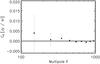 |
Fig. 4 Mean cross-power spectrum of 500 FIRB random maps at 857 GHz with the LRG map; the signal is perfectly compatible with zero. |
We also performed a rotation test (Sawangwit et al. 2010; Giannantonio et al. 2012), where one of the maps is rotated by an arbitrary angle and then cross-correlated with the other map: if the rotation angle Δφ is large enough, and in absence of systematics, the resulting cross-power spectrum should be compatible with zero. Keeping the FIRB map mixed, we computed N = 89 cross-power spectra with N galaxy maps, rotated by Δφ = 4 degrees with respect to each other and used the corresponding rotated galaxy masks; with χ2 = 16.5 for 9 degrees of freedom, we accept the null-test hypothesis of correlation consistent with zero.
3.3. Analysis and results
In Fig. 5, we show the cross-power spectra measured for the four frequencies considered and with the uncertainty computed from Monte Carlo simulations. The statistical significance of the signal is obtained by summing, for each frequency ν, the significance in the different multipole bins i as  (19)we obtain values of 8.7, 13.0, 12.3, and 12.6 at 3000, 857, 545, and 353 GHz, respectively.
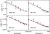 |
Fig. 5 Cross-power spectra measurements among CIB maps at 3000, 857, 545, and 353 GHz, and CMASS LRGs (black points); for the IRIS 3000 GHz channel we did not use data points at multipoles l > 500. Best-fit power spectra are shown for the parametric SED functional form (red lines) and for the effective SED (blue dashed-dotted lines). |
The theoretical cross-power spectrum is given by Eq. (12) and a Poisson term, because of far-infrared emission from individual galaxies, is not included, because for the LRG’s number density and average FIR emission, it is negligible. The redshift distribution of FIRB sources at the observed frequency ν is connected to the mean FIRB emissivity per comoving unit volume jν(z) through the relation  (20)where the galaxy emissivity
  can be written as
  (21)here L(1 + z)ν and dn/ dL denote the infrared galaxy luminosity and luminosity function, respectively, while the term (1 + z)ν denotes the rest-frame frequency. The emissivity jν(z) is modeled with a halo-model approach, introduced in Shang et al. (2012) and successfully applied in, e.g., Planck Collaboration XXX (2014); Viero et al. (2013), whose main feature is the introduction of a parametric form to describe the dependence of the galaxy luminosity on its host halo mass. This allows us to overcome the unrealistic assumption, typical of many models based on a set of infrared luminosity functions and a prescription to populate galaxies in dark matter halos using a halo occupation distribution (HOD) formalism that galaxies have all the same luminosity and contribute to the emissivity density in the same way, despite their dark matter environment. Shang et al. (2012) provide a detailed description of the theoretical motivations and limitations of the modeling.
In this model, the galaxy infrared luminosity L(1 + z)ν is linked to the host dark matter halo mass using the following parametric form: ![Mathematical equation: \begin{equation} L_{(1\,+\,z)\nu}(M,z)=L_0 \left(1\,+\,z\right)^{3.6} \Sigma(M) \Theta[(1\,+\,z)\nu] \label{eqn:lfunc} \end{equation}](/articles/aa/full_html/2014/10/aa23958-14/aa23958-14-eq128.png) (22)where the redshift-dependent, global normalization, has been fixed to the mean value found in Planck Collaboration XXX (2014), while the term L0 is a normalization parameter constrained with the CIB mean level at the frequencies considered. We will not discuss this parameter further in the rest of our analysis.
(22)where the redshift-dependent, global normalization, has been fixed to the mean value found in Planck Collaboration XXX (2014), while the term L0 is a normalization parameter constrained with the CIB mean level at the frequencies considered. We will not discuss this parameter further in the rest of our analysis.
We also assume a log-normal function Σ(M) for the dependence of the galaxy luminosity on halo mass  (23)where Meff and σL/M describe the peak of the specific IR emissivity and the range of halo masses which is more efficient at producing star formation; following Shang et al. (2012); Planck Collaboration XXX (2014), we assume the condition
  while we fix the minimum halo mass at Mmin = 1010 M⊙ (compatible with Viero et al. 2013) throughout this paper. The log-normal functional form used here describes the observation that a limited range of halo masses dominates the star formation activity. Recent cosmological simulations suggest that processes such as photoionization, supernovae heating, feedback from active galactic nuclei, and virial shocks suppress star formation at both the low- and the high-mass end (Benson et al. 2003; Croton et al. 2006; Silk 2003; Bertone et al. 2005; Birnboim & Dekel 2003; Kereš et al. 2005; Dekel & Birnboim 2006); it is thus possible to introduce a characteristic mass scale Meff, which phenomenologically illustrates the impact of dark matter on star formation processes.
In general, a modified back body functional form (see Blain et al. 2003, and reference therein) can be assumed for galaxy SEDs  (24)where Bν denotes the Planck function, while the emissivity index β gives information about the physical nature of dust, in general depending on grain composition, temperature distribution of tunneling states and wavelength-dependent excitation (e.g., Meny et al. 2007). The power-law function is used to temper the exponential (Wien) tail at high frequencies and obtain a shallower SED shape, which is more in agreement with observed SEDs (see, e.g., Blain et al. 2003). The two SED functions at high and low frequencies are connected smoothly at the frequency ν0 satisfying
  (25)We explicitly checked that our data do not allow us to strongly constrain the emissivity index β and the SED parameter γ; thus, we fixed their values to the mean values found by Planck Collaboration XXX (2014), as β = 1.7 and γ = 1.7. Finally, the parameter Td describes the average dust temperature of FIRB sources at z ~ 0.55. Note that, since our measurement is restricted to quite a narrow redshift bin, we do not consider a possible redshift dependence of parameters such as Meff or Td; the only redshift-dependent quantity is the global normalization term Φ(z).
The parameter space is sampled using a Monte Carlo Markov chain analysis with a modified version of the publicly available code CosmoMC (Lewis & Bridle 2002). We consider variations in the following set of three halo model parameters:  (26)we assume the following priors on our physical parameters: log (Meff) ∈ [ 11:13 ] M⊙ and Td ∈ [ 20:60 ] K, and we explicitly checked that our results do not depend on the priors assumed.
Mean values and marginalized 68% c.l. for halo model parameters.
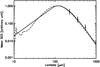 |
Fig. 6 Best-fit SEDs at z = 0.55 (both normalized to have amplitude equal to one at λ = 120 μm) computed with the modified blackbody functional form (continuous line) and with the mean effective SED approach (dot-dash line), as in Béthermin et al. (2012a). Data points show a (normalized) estimate for the SED of FIRB fluctuations computed from the ratio of the cross-power spectra at multipole l = 450. |
In addition to fitting to the four cross-power spectra, we also use the mean level of the CIB at 3000 GHz ( nW m-2sr-1), 857 GHz (
 nW m-2 sr-1) and 545 GHz (
 nW m-2sr-1) deduced from galaxy number counts as useful priors to constrain the global normalization parameter L0.
Our set of three parameters allows us to obtain a very good fit to the data (Fig. 5), with a best-fit χ2 of 26.9 for 31 degrees of freedom. Mean values and marginalized limits on the halo-model parameters considered here are listed in Table 1. They are in good agreement with results obtained from the analysis of Planck and IRIS auto-power spectra using the same parameterization for the FIRB emissivity in Planck Collaboration XXX 2014, providing a strong confirmation of their results.
Using the values in Table 1, we also compute the approximate fraction of the total FIRB responsible for the cross-correlation with LRGs, obtaining 11.8% at 3000 GHz, 3.9% at 857 GHz, 1.8% at 545 GHz, and 1% at 353 GHz. Compatible results are obtained through the computation of the mean coherence (Kashlinsky et al. 2012; Cappelluti et al. 2013) of the signal, defined as the square of the ratio of the cross-power spectra to the geometric mean of the auto-power spectra:  (27)Finally, the mean values inferred for both the dust temperature (Td = 26.0 ± 1.3 K) and the bias (bFIRB ~ 1.45) are compatible with results obtained by Planck Collaboration XXX (2014) at z ≃ 0.55.
To test the robustness of our results, we also replaced our parametric SED functional form with the mean effective SED Sν,eff of all galaxies at redshift z = 0.55 from Béthermin et al. (2012a), and we repeated the analysis, keeping only Meff and L0 as free parameters. With a  of 1.0 (best-fit χ2 equal to 31.9 for 32 degrees of freedom) our fit is satisfying; however, the most efficient halo mass at hosting star-forming galaxies is Meff = 12.90 ± 0.14, higher than Planck Collaboration XXX (2014), and compatible at 95% c.l.
As we can see in Fig. 6, the parametric form used in this paper is similar to the mean effective SED for the range of wavelengths that matters in this analysis, yielding a satisfactory confirmation of the goodness of our results. However, the γ parameter, which controls the high frequency tail of the spectrum, fails to correctly reproduce the shape of real galaxy SEDs in the mid-infrared regime (from 10 to 30μm), mainly because of broad line absorption from polycyclic aromatic hydrocarbon (PAH) molecules. In Fig. 6, we also plot the value of the FIRB SED computed from the ratio of the measured cross-power spectra at multipole l = 450 and shifted to redshift z = 0.55; our results are compatible with the best-fit SEDs used in the paper.
On linear scales, the cross-power spectra considered can also be fitted by power laws. Assuming a simple, two-parameter functional form such as  (28)it is possible to obtain a very good fit at all frequencies over the multipole range 100 < l < 500. Mean values and marginalized limits on the amplitudes Aν and power-law slopes nν are provided in Table 2.
Mean values and marginalized 68% c.l. for power-law parameters.
3.4. Discussion
As mentioned earlier, the dark matter halo mass influences the evolution of galaxies, driving processes of gas accretion and star formation rate (SFR; see, e.g., Rees & Ostriker 1977; Silk 1977; White & Rees 1978; Fall & Efstathiou 1980; Blumenthal et al. 1984). Numerous techniques have been considered to constrain the link between dark matter halos and their host galaxies (see discussion and references in Behroozi et al. 2010; Moster et al. 2010). From a theoretical point of view, semi analytic models and hydrodynamical simulations have been developed to study galaxy formation processes ab initio; however, they are still not able to reproduce many observational evidences and suffer from several uncertainties. A different approach, which does not rely on assumptions related to poorly constrained physical processes and is based instead on a statistical description of the link between galaxies and dark matter, is the basis for the HOD formalism and the abundance matching technique, which also assumes the existence of a monotonic relation between halo mass and galaxy stellar mass. Results based on abundance matching, applied to optical and infrared data (Béthermin et al. 2012b; Behroozi et al. 2012; Moster et al. 2010; Guo et al. 2010), constrain the characteristic halo mass at Meff ~ 1012 M⊙, with little evolution in redshift and some uncertainty, mainly due to systematics in the stellar mass estimates (Behroozi et al. 2010). The higher value obtained in this work (Meff ~ 6.9 × 10¹² M⊙), can be due to the adoption of a log-normal function to model the luminosity-mass relation, while the previously mentioned analyses use a more complicated relation, to take the slow decrease of the stellar mass to halo mass ratio at the high mass end into account. However, the mean value for the most efficient mass found here is in agreement with, or only slightly higher than, results from recent analyses of FIRB anisotropies (Shang et al. 2012; Xia et al. 2012; Viero et al. 2013; Planck Collaboration XXX 2014).
We note that the narrow redshift bin involved in our analysis imposes the use of a very simple interpretative model for both the LRGs and the FIRB galaxies. In particular, both the redshift evolution of the galaxy FIR luminosity and some SED parameters are kept fixed. In an upcoming study, we will cross-correlate FIRB anisotropies with a combination of data from multiple surveys such as WISE, GALEX, and BOSS. This will allow us to probe the link between dark matter and galaxies over a wide redshift range, from low redshifts (0 < z < 1) where a steep evolution of the cosmic star formation has been measured, to high redshifts (1 < z < 3), where the SFR peaks. Introducing redshift-dependent quantities and a realistic scatter in the relation between galaxy luminosity and dark matter halo mass (that has been neglected here, see discussion in Shang et al. 2012), we will be able to study the temporal evolution of the most efficient halo mass at hosting star formation (possibly constraining downsizing scenarios, Cowie et al. 1996; Bundy et al. 2006; Conroy & Wechsler 2009), thus establishing cross-correlations with FIRB anisotropies as a powerful probe of the link between galaxies and dark matter and the global star formation history.
4. Conclusions
We have measured the cross-correlation between LRGs from SDSS-III DR8 and CIB anisotropies from IRIS and Planck at 3000, 857, 545, and 353 GHz. Using an extended version of the halo model that connects galaxy luminosity to host halo mass with a simple parametric form, we confirmed the basic results obtained from recent analyses of FIRB anisotropies from Planck and Herschel, with a most efficient halo mass at hosting star-forming galaxies constrained at the value log (Meff/M⊙) = 12.84 ± 0.15, and the mean dust temperature of FIR sources at z ~ 0.55 with the value Td = 26.0 ± 1.3K.
The cross-correlation of FIRB sources with other tracers of the dark matter field now starts being successfully exploited to constrain the interplay between dark and luminous matter (see, e.g., Wang et al. 2014), and cross-correlations with data from present and upcoming surveys are particularly promising for many reasons. First of all, while the measurement of FIRB auto-power spectra will not improve much in the near future, as they are limited by issues related to components separation, cross-correlations with FIRB anisotropies are limited mostly by noise and systematics. In particular, control of the effects of Galactic dust will be critical to achieving a precise measurement of the cross-correlation, since it contributes significantly to the total uncertainty. Dust subtraction, using ancillary data and clean regions of the sky (as done in Planck Collaboration XXX 2014) can improve the signal-to-noise ratio, provided that large enough fields are considered. A careful analysis of systematics is also mandatory to exclude the possibility of correlated systematics between datasets; an example is stellar density affecting quasar catalogs and Galactic dust affecting FIRB anisotropies, which correlate and contaminate the cross-correlation signal.
Cross-correlations with FIRB anisotropies are also important because they allow us to isolate the CIB signal in multiple redshift slices and thus constrain the link between galaxies and dark matter and global star formation as a function of redshift. These studies will be particularly interesting when performed with sources at high redshift (such as, e.g., quasars from BOSS), where the cosmic SFR peaks and current model uncertainties for DSFGs are large.
The mask can be found at http://pla.esac.esa.int/pla/aio/planckResults.jsp? with CATEGORY = MASK_gal−06
Acknowledgments
The development of Planck has been supported by: ESA; CNES and CNRS/INSU-IN2P3-INP (France); ASI, CNR, and INAF (Italy); NASA and DoE (USA); STFC and UKSA (UK); CSIC, MICINN and JA (Spain); Tekes, AoF and CSC (Finland); DLR and MPG (Germany); CSA (Canada); DTU Space (Denmark); SER/SSO (Switzerland); RCN (Norway); SFI (Ireland); FCT/MCTES (Portugal); and PRACE (EU). A description of the Planck Collaboration and a list of its members, including the technical or scientific activities in which they have been involved, can be found at http://www.sciops.esa.int/index.php?project=planck&page=Planck_Collaboration. We would like to thank the anonymous referee for providing us with constructive comments and suggestions. P.S. would like to thank Alex Amblard and Shirley Ho for useful discussions. Part of the research described in this paper was carried out at the Jet Propulsion Laboratory, California Institute of Technology, under a contract with the National Aeronautics and Space Administration.
References
- Amblard, A., Cooray, A., Serra, P., et al. 2011, Nature, 470, 510 [NASA ADS] [CrossRef] [Google Scholar]
- Behroozi, P. S., Conroy, C., & Wechsler, R. H. 2010, ApJ, 717, 379 [NASA ADS] [CrossRef] [Google Scholar]
- Behroozi, P. S., Wechsler, R. H., & Conroy, C. 2012, arXiv e-prints [Google Scholar]
- Benson, A. J., Bower, R. G., Frenk, C. S., et al. 2003, ApJ, 599, 38 [NASA ADS] [CrossRef] [Google Scholar]
- Bertone, S., Stoehr, F., & White, S. D. M. 2005, MNRAS, 359, 1201 [NASA ADS] [CrossRef] [Google Scholar]
- Béthermin, M., Daddi, E., Magdis, G., et al. 2012a, ApJ, 757, L23 [NASA ADS] [CrossRef] [Google Scholar]
- Béthermin, M., Doré, O., & Lagache, G. 2012b, A&A, 537, L5 [NASA ADS] [CrossRef] [EDP Sciences] [Google Scholar]
- Birnboim, Y., & Dekel, A. 2003, MNRAS, 345, 349 [NASA ADS] [CrossRef] [Google Scholar]
- Blain, A. W., Barnard, V. E., & Chapman, S. C. 2003, MNRAS, 338, 733 [NASA ADS] [CrossRef] [Google Scholar]
- Blumenthal, G. R., Faber, S. M., Primack, J. R., & Rees, M. J. 1984, Nature, 311, 517 [NASA ADS] [CrossRef] [Google Scholar]
- Bundy, K., Ellis, R. S., Conselice, C. J., et al. 2006, ApJ, 651, 120 [NASA ADS] [CrossRef] [Google Scholar]
- Cappelluti, N., Kashlinsky, A., Arendt, R. G., et al. 2013, ApJ, 769, 68 [NASA ADS] [CrossRef] [Google Scholar]
- Conroy, C., & Wechsler, R. H. 2009, ApJ, 696, 620 [NASA ADS] [CrossRef] [Google Scholar]
- Cooray, A., & Sheth, R. 2002, Phys. Rep., 372, 1 [NASA ADS] [CrossRef] [Google Scholar]
- Cowie, L. L., Songaila, A., Hu, E. M., & Cohen, J. G. 1996, AJ, 112, 839 [Google Scholar]
- Croton, D. J., Springel, V., White, S. D. M., et al. 2006, MNRAS, 365, 11 [NASA ADS] [CrossRef] [Google Scholar]
- de Putter, R., Mena, O., Giusarma, E., et al. 2012, ApJ, 761, 12 [NASA ADS] [CrossRef] [Google Scholar]
- Dekel, A., & Birnboim, Y. 2006, MNRAS, 368, 2 [NASA ADS] [CrossRef] [Google Scholar]
- Dole, H., Lagache, G., Puget, J. L., et al. 2006, A&A, 451, 417 [NASA ADS] [CrossRef] [EDP Sciences] [MathSciNet] [Google Scholar]
- Dunkley, J., Hlozek, R., Sievers, J., et al. 2011, ApJ, 739, 52 [NASA ADS] [CrossRef] [Google Scholar]
- Eisenstein, D. J., Weinberg, D. H., Agol, E., et al. 2011, AJ, 142, 72 [Google Scholar]
- Fall, S. M., & Efstathiou, G. 1980, MNRAS, 193, 189 [NASA ADS] [CrossRef] [Google Scholar]
- Fixsen, D. J., Dwek, E., Mather, J. C., Bennett, C. L., & Shafer, R. A. 1998, ApJ, 508, 123 [NASA ADS] [CrossRef] [Google Scholar]
- Giannantonio, T., Scranton, R., Crittenden, R. G., et al. 2008, Phys. Rev. D, 77, 123520 [NASA ADS] [CrossRef] [Google Scholar]
- Giannantonio, T., Crittenden, R., Nichol, R., & Ross, A. J. 2012, MNRAS, 426, 2581 [NASA ADS] [CrossRef] [Google Scholar]
- Górski, K. M., Hivon, E., Banday, A. J., et al. 2005, ApJ, 622, 759 [NASA ADS] [CrossRef] [Google Scholar]
- Guo, Q., White, S., Li, C., & Boylan-Kolchin, M. 2010, MNRAS, 404, 1111 [NASA ADS] [Google Scholar]
- Hall, N. R., Keisler, R., Knox, L., et al. 2010, ApJ, 718, 632 [NASA ADS] [CrossRef] [Google Scholar]
- Hauser, M. G., Arendt, R. G., Kelsall, T., et al. 1998, ApJ, 508, 25 [NASA ADS] [CrossRef] [Google Scholar]
- Hivon, E., Górski, K. M., Netterfield, C. B., et al. 2002, ApJ, 567, 2 [NASA ADS] [CrossRef] [Google Scholar]
- Ho, S., Cuesta, A., Seo, H.-J., et al. 2012, ApJ, 761, 14 [NASA ADS] [CrossRef] [Google Scholar]
- Kashlinsky, A., & Odenwald, S. 2000, ApJ, 528, 74 [NASA ADS] [CrossRef] [Google Scholar]
- Kashlinsky, A., Odenwald, S., Mather, J., Skrutskie, M. F., & Cutri, R. M. 2002, ApJ, 579, L53 [NASA ADS] [CrossRef] [Google Scholar]
- Kashlinsky, A., Arendt, R. G., Mather, J., & Moseley, S. H. 2005, Nature, 438, 45 [NASA ADS] [CrossRef] [PubMed] [Google Scholar]
- Kashlinsky, A., Arendt, R. G., Ashby, M. L. N., et al. 2012, ApJ, 753, 63 [NASA ADS] [CrossRef] [Google Scholar]
- Kereš, D., Katz, N., Weinberg, D. H., & Davé, R. 2005, MNRAS, 363, 2 [NASA ADS] [CrossRef] [Google Scholar]
- Lagache, G., Abergel, A., Boulanger, F., Désert, F. X., & Puget, J.-L. 1999, A&A, 344, 322 [NASA ADS] [Google Scholar]
- Lagache, G., & Puget, J. L. 2000, A&A, 355, 17 [NASA ADS] [Google Scholar]
- Lagache, G., Haffner, L. M., Reynolds, R. J., & Tufte, S. L. 2000, A&A, 354, 247 [Google Scholar]
- Lagache, G., Bavouzet, N., Fernandez-Conde, N., et al. 2007, ApJ, 665, L89 [NASA ADS] [CrossRef] [Google Scholar]
- Lewis, A., & Bridle, S. 2002, Phys. Rev. D, 66, 103511 [NASA ADS] [CrossRef] [Google Scholar]
- Limber, D. N. 1953, ApJ, 117, 134 [NASA ADS] [CrossRef] [Google Scholar]
- Matsuhara, H., Kawara, K., Sato, Y., et al. 2000, A&A, 361, 407 [NASA ADS] [Google Scholar]
- Matsumoto, T., Matsuura, S., Murakami, H., et al. 2005, ApJ, 626, 31 [NASA ADS] [CrossRef] [Google Scholar]
- Ménard, B., Scranton, R., Schmidt, S., et al. 2013, arXiv e-prints [Google Scholar]
- Meny, C., Gromov, V., Boudet, N., et al. 2007, A&A, 468, 171 [Google Scholar]
- Miville-Deschênes, M.-A., & Lagache, G. 2005, ApJS, 157, 302 [NASA ADS] [CrossRef] [Google Scholar]
- Miville-Deschênes, M.-A., Lagache, G., & Puget, J.-L. 2002, A&A, 393, 749 [NASA ADS] [CrossRef] [EDP Sciences] [Google Scholar]
- Moster, B. P., Somerville, R. S., Maulbetsch, C., et al. 2010, ApJ, 710, 903 [NASA ADS] [CrossRef] [Google Scholar]
- Navarro, J. F., Frenk, C. S., & White, S. D. M. 1997, ApJ, 490, 493 [NASA ADS] [CrossRef] [Google Scholar]
- Pâris, I., Petitjean, P., Aubourg, É., et al. 2014, A&A, 563, A54 [NASA ADS] [CrossRef] [EDP Sciences] [Google Scholar]
- Planck Collaboration XVIII. 2011, A&A, 536, A18 [NASA ADS] [CrossRef] [EDP Sciences] [Google Scholar]
- Planck Collaboration I. 2014, A&A, 571, A1 [NASA ADS] [CrossRef] [EDP Sciences] [Google Scholar]
- Planck Collaboration VI. 2014, A&A, 571, A6 [NASA ADS] [CrossRef] [EDP Sciences] [Google Scholar]
- Planck Collaboration VII. 2014, A&A, 571, A7 [NASA ADS] [CrossRef] [EDP Sciences] [Google Scholar]
- Planck Collaboration VIII. 2014, A&A, 571, A8 [NASA ADS] [CrossRef] [EDP Sciences] [Google Scholar]
- Planck Collaboration XVI. 2014, A&A, 571, A16 [NASA ADS] [CrossRef] [EDP Sciences] [Google Scholar]
- Planck Collaboration XVIII. 2014, A&A, 571, A18 [NASA ADS] [CrossRef] [EDP Sciences] [Google Scholar]
- Planck Collaboration XXVIII. 2014, A&A, 571, A28 [NASA ADS] [CrossRef] [EDP Sciences] [Google Scholar]
- Planck Collaboration XXX. 2014, A&A, 571, A30 [NASA ADS] [CrossRef] [EDP Sciences] [Google Scholar]
- Puget, J.-L., Abergel, A., Bernard, J.-P., et al. 1996, A&A, 308, L5 [NASA ADS] [Google Scholar]
- Rees, M. J., & Ostriker, J. P. 1977, MNRAS, 179, 541 [NASA ADS] [CrossRef] [Google Scholar]
- Reichardt, C. L., Shaw, L., Zahn, O., et al. 2012, ApJ, 755, 70 [NASA ADS] [CrossRef] [Google Scholar]
- Ross, A. J., Ho, S., Cuesta, A. J., et al. 2011, MNRAS, 417, 1350 [NASA ADS] [CrossRef] [Google Scholar]
- Sawangwit, U., Shanks, T., Cannon, R. D., et al. 2010, MNRAS, 402, 2228 [NASA ADS] [CrossRef] [Google Scholar]
- Shang, C., Haiman, Z., Knox, L., & Oh, S. P. 2012, MNRAS, 421, 2832 [NASA ADS] [CrossRef] [Google Scholar]
- Silk, J. 1977, ApJ, 211, 638 [NASA ADS] [CrossRef] [Google Scholar]
- Silk, J. 2003, MNRAS, 343, 249 [NASA ADS] [CrossRef] [MathSciNet] [Google Scholar]
- Smith, R. E., Peacock, J. A., Jenkins, A., et al. 2003, MNRAS, 341, 1311 [NASA ADS] [CrossRef] [Google Scholar]
- Tinker, J., Kravtsov, A. V., Klypin, A., et al. 2008, ApJ, 688, 709 [NASA ADS] [CrossRef] [Google Scholar]
- Tinker, J. L., Robertson, B. E., Kravtsov, A. V., et al. 2010, ApJ, 724, 878 [NASA ADS] [CrossRef] [Google Scholar]
- Viero, M. P., Ade, P. A. R., Bock, J. J., et al. 2009, ApJ, 707, 1766 [NASA ADS] [CrossRef] [Google Scholar]
- Viero, M. P., Wang, L., Zemcov, M., et al. 2013, ApJ, 772, 77 [NASA ADS] [CrossRef] [Google Scholar]
- Wang, L., Viero, M., Ross, N. P., et al. 2014, arXiv e-prints [Google Scholar]
- White, S. D. M., & Rees, M. J. 1978, MNRAS, 183, 341 [NASA ADS] [CrossRef] [Google Scholar]
- White, M., Blanton, M., Bolton, A., et al. 2011, ApJ, 728, 126 [NASA ADS] [CrossRef] [Google Scholar]
- Wright, E. L., Eisenhardt, P. R. M., Mainzer, A. K., et al. 2010, AJ, 140, 1868 [NASA ADS] [CrossRef] [Google Scholar]
- Xia, J.-Q., Negrello, M., Lapi, A., et al. 2012, MNRAS, 422, 1324 [NASA ADS] [CrossRef] [Google Scholar]
All Tables
All Figures
|
Fig. 1 Normalized SDSS-III DR8 LRG redshift distribution, peaked at |
| In the text | |
|
Fig. 2 Angular auto-power spectrum measured in the SDSS-III DR8 LRG survey. |
| In the text | |
|
Fig. 3 Apodized mask used to cross-correlate the DR8 LRG map with the Planck temperature map at 857 GHz; the sky fraction unmasked is approximately fsky = 0.185. |
| In the text | |
|
Fig. 4 Mean cross-power spectrum of 500 FIRB random maps at 857 GHz with the LRG map; the signal is perfectly compatible with zero. |
| In the text | |
|
Fig. 5 Cross-power spectra measurements among CIB maps at 3000, 857, 545, and 353 GHz, and CMASS LRGs (black points); for the IRIS 3000 GHz channel we did not use data points at multipoles l > 500. Best-fit power spectra are shown for the parametric SED functional form (red lines) and for the effective SED (blue dashed-dotted lines). |
| In the text | |
|
Fig. 6 Best-fit SEDs at z = 0.55 (both normalized to have amplitude equal to one at λ = 120 μm) computed with the modified blackbody functional form (continuous line) and with the mean effective SED approach (dot-dash line), as in Béthermin et al. (2012a). Data points show a (normalized) estimate for the SED of FIRB fluctuations computed from the ratio of the cross-power spectra at multipole l = 450. |
| In the text | |
Current usage metrics show cumulative count of Article Views (full-text article views including HTML views, PDF and ePub downloads, according to the available data) and Abstracts Views on Vision4Press platform.
Data correspond to usage on the plateform after 2015. The current usage metrics is available 48-96 hours after online publication and is updated daily on week days.
Initial download of the metrics may take a while.