| Issue |
A&A
Volume 570, October 2014
|
|
|---|---|---|
| Article Number | A88 | |
| Number of page(s) | 15 | |
| Section | Stellar atmospheres | |
| DOI | https://doi.org/10.1051/0004-6361/201423842 | |
| Published online | 22 October 2014 | |
Weak magnetic fields in central stars of planetary nebulae?⋆
1 Leibniz-Institut für Astrophysik Potsdam, An der Sternwarte 16, 14482 Potsdam, Germany
e-mail: msteffen@aip.de
2 Universität Potsdam, Institut für Physik und Astronomie, 14476 Potsdam, Germany
3 European Southern Observatory, Karl-Schwarzschild-Str. 2, 85748 Garching, Germany
Received: 19 March 2014
Accepted: 13 August 2014
Context. It is not yet clear whether magnetic fields play an essential role in shaping planetary nebulae (PNe), or whether stellar rotation alone and/or a close binary companion, stellar or substellar, can account for the variety of the observed nebular morphologies.
Aims. In a quest for empirical evidence verifying or disproving the role of magnetic fields in shaping planetary nebulae, we follow up on previous attempts to measure the magnetic field in a representative sample of PN central stars.
Methods. We obtained low-resolution polarimetric spectra with FORS 2 installed on the Antu telescope of the VLT for a sample of 12 bright central stars of PNe with different morphologies, including two round nebulae, seven elliptical nebulae, and three bipolar nebulae. Two targets are Wolf-Rayet type central stars.
Results. For the majority of the observed central stars, we do not find any significant evidence for the existence of surface magnetic fields. However, our measurements may indicate the presence of weak mean longitudinal magnetic fields of the order of 100 Gauss in the central star of the young elliptical planetary nebula IC 418 as well as in the Wolf-Rayet type central star of the bipolar nebula Hen 2-113 and the weak emission line central star of the elliptical nebula Hen 2-131. A clear detection of a 250 G mean longitudinal field is achieved for the A-type companion of the central star of NGC 1514. Some of the central stars show a moderate night-to-night spectrum variability, which may be the signature of a variable stellar wind and/or rotational modulation due to magnetic features.
Conclusions. Since our analysis indicates only weak fields, if any, in a few targets of our sample, we conclude that strong magnetic fields of the order of kG are not widespread among PNe central stars. Nevertheless, simple estimates based on a theoretical model of magnetized wind bubbles suggest that even weak magnetic fields below the current detection limit of the order of 100 G may well be sufficient to contribute to the shaping of the surrounding nebulae throughout their evolution. Our current sample is too small to draw conclusions about a correlation between nebular morphology and the presence of stellar magnetic fields.
Key words: planetary nebulae: general / stars: magnetic field / stars: AGB and post-AGB / binaries: close / techniques: polarimetric
© ESO, 2014
1. Introduction
One of the major open questions regarding the formation of planetary nebulae (PNe) concerns the mechanism that is responsible for their non-spherical, often axisymmetric shaping (e.g., review by Balick & Frank 2002). Both central star binarity and stellar rotation in combination with magnetic fields are among the favorite explanations, but their role in PN formation and shaping is not yet sufficiently clear.
Basically, the origin of PNe is understood to be a consequence of the interaction of the hot central star with its circumstellar environment through photoionization and wind-wind collision. In the framework of this theory, the formation and evolution of PNe has been modeled in detail, assuming spherical symmetry (e.g., Marten & Schönberner 1991; Mellema 1994; Villaver at al. 2002; Perinotto et al. 2004; Steffen & Schönberner 2006) or axisymmetric geometry (e.g., Mellema 1995; 1997). The role of stellar rotation and magnetic fields in shaping PNe has been studied numerically in the pioneering work of García-Segura et al. (1999), who find that most of the observed nebular morphologies can be modeled with an appropriate combination of input parameters. Magnetic shaping of PNe thus appears to be an attractive alternative to the popular binary hypothesis (e.g., De Marco 2009; Douchin et al. 2012). It remains unclear, however, whether the underlying assumptions of García-Segura et al. (constant stellar wind with a high magnetization parameter) are actually realistic, since very little is known so far about rotation rates and surface magnetic fields of the central stars of PNe.
The discovery of sufficiently strong magnetic fields in the central stars would lend considerable support to the hypothesis that the axisymmetric or bipolar appearance of many PNe is caused by magnetic fields (e.g., García-Díaz et al. 2008; Blackman 2009). On the other hand, theoretical arguments have been put forward to demonstrate that the structure of non-spherical planetary nebulae cannot be attributed to the presence of large scale magnetic fields, since they would contain more angular momentum and energy than a single star can supply (Soker 2006).
List of PNe central stars observed in the framework of our program, ordered by increasing RA.
In principle, the role of magnetic fields in shaping PNe may be verified or disproved by empirical evidence, as already suggested by Jordan et al. (2005). Using FORS 1 in spectropolarimetric mode, they reported the detection of magnetic fields of the order of kG in the central stars of the PNe NGC 1360 and LSS 1362. A reanalysis of their data, however, did not provide any significant evidence for longitudinal magnetic fields in these stars that are stronger than a few hundred Gauss (Jordan et al. 2012). Their field measurements have typical error bars of 150 to 300 G. Similar results were achieved in the work of Leone et al. (2011), who concluded that the mean longitudinal magnetic fields in NGC 1360 and LSS 1362 are much weaker, less than 600 G, or that the field has a complex structure. The most recent search for magnetic fields in central stars of planetary nebulae by Leone et al. (2014), based on spectropolarimetric observations of 19 central stars with WHT/ISIS and VLT/FORS 2, is partly affected by large measurement uncertainties and reports no positive detection either. Thus, convincing evidence for the presence of significant magnetic fields in the central stars of PNe is still missing.
Using low-resolution polarimetric spectra obtained with FORS 2 installed at the Very Large Telescope (VLT), we carried out a search for magnetic fields in a sample of 12 central stars covering the whole range of morphologies from round to elliptical/axisymmetric, and bipolar PNe, and including both chemically normal and Wolf-Rayet (WR) type (hydrogen-poor) central stars. The sample includes two round nebulae (NGC 246, Hen 2-108), five elliptical nebulae (IC 418, NGC 1514, NGC 2392, NGC 3132, Hen 2-131), and three bipolar nebulae (NGC 2346, Hen 2-36, Hen 2-113). Two targets are WR-type central stars (NGC 246, Hen 2-113). In addition, we included the two (elliptical) targets of Jordan et al. (2005), NGC 1360 and LSS 1362, for which they originally claimed the detection of kG magnetic fields. Six of the 12 central stars are known binaries.
The data collected in our survey can provide a basis for further empirical investigations. Since our sample comprises both normal hydrogen-burning, and Wolf-Rayet type (hydrogen-deficient) central stars, some insight may be gained into the physics of WR-type winds regarding the question of whether the much enhanced mass loss of [WC] type central stars (by a factor of ~100 with respect to the mass loss of normal central stars) is related to the presence of stellar magnetic fields.
Our target list includes a number of nebulae whose X-ray emission has been measured by Chandra and/or XMM Newton or are prospective targets in the Chandra PN large project (PI J. Kastner). In principle, our magnetic field measurements may help to answer the question why some central stars show up as X-ray point sources, while others, with similar stellar parameters, do not emit X-rays. The magnetic properties of the central stars and their winds could play an important role in this context. Similarly, the central cavity of some PNe is known to be a source of diffuse thermal X-ray emission, while other PNe are undetected in diffuse X-rays. Again, magnetic fields may be responsible: (i) sufficiently strong magnetic fields are expected to modify the thermal structure of the shock-heated stellar wind, and hence its X-ray emission; and (ii) even very weak magnetic fields suppress thermal conduction perpendicular to the field lines, with severe consequences for the X-ray luminosity and characteristic temperature (Steffen et al. 2008).
In Sect. 2, we give an overview of our observations and magnetic field measurements with VLT/FORS 2, before we discuss the main results of our 12 targets in Sect. 3. Section 4 is devoted to theoretical estimates of the role of the central star’s magnetic fields in PN shaping and of the influence of the magnetic fields on the diffuse X-ray emission of PNe. Finally, we summarize our main conclusions in Sect. 5.
2. Observations and magnetic field measurements
Spectropolarimetric observations of 12 central stars were carried out from 2011 October 5 to 2012 March 28 in service mode at the European Southern Observatory with FORS 2 mounted on the 8 m Antu telescope of the VLT. Nine targets were observed twice, and three targets were observed three times. We present the list of targets in our sample in Table 1, where we also collect information about the spectral classification of the central stars, binarity, morphology of the nebulae, and observed X-ray emission.
The multi-mode instrument FORS 2 is equipped with polarization analyzing optics, comprising superachromatic halfwave and quarterwave phase retarder plates, and a Wollaston prism with a beam divergence of 22″ in standard resolution mode. During the observations with FORS 2, we used a slit width of 0.̋5 and the GRISM 600B to achieve a spectral resolving power of about 1650.
From the raw FORS 2 data, the parallel and perpendicular beams are extracted using a pipeline written in the MIDAS environment by T. Szeifert, the very first FORS instrument scientist. This pipeline reduction by default includes background subtraction. A unique wavelength calibration frame is used for each night.
A first description of the assessment of the longitudinal magnetic field measurements using FORS 1/2 spectropolarimetric observations was presented in our previous work (e.g., Hubrig et al. 2004a; 2004b, and references therein). To minimize the crosstalk effect, a sequence of subexposures at the retarder position angles −45° + 45°, + 45° − 45°, −45° + 45°, etc., is usually executed during observations and the V/I spectrum is calculated using:  (1)where + 45° and −45° indicate the position angle of the retarder waveplate and fo and fe are the ordinary and extraordinary beams, respectively. Rectification of the V/I spectra was performed in the way described by Hubrig et al. (2014). Null profiles, N, are calculated as pairwise differences from all available V profiles. From these, 3σ-outliers are identified and used to clip the V profiles. This removes spurious signals, which mostly come from cosmic rays and also reduces the noise. A full description of the updated data reduction and analysis will be presented in a separate paper (Schöller et al., in prep.).
The mean longitudinal magnetic field, ⟨Bz⟩, is measured on the rectified and clipped spectra based on the relation  (2)where V is the Stokes parameter that measures the circular polarization, I is the intensity in the unpolarized spectrum, geff is the effective Landé factor, e is the electron charge, λ is the wavelength, me is the electron mass, c is the speed of light, dI/ dλ is the wavelength derivative of Stokes I, and ⟨Bz⟩ is the mean longitudinal (line-of-sight) magnetic field.
For the determination of the mean longitudinal stellar magnetic field, we consider two sets of spectral lines: (i) the entire spectrum including all available absorption and emission lines, apart from the usually strong [O iii] nebula emission lines near 5000 Å (in the following referred to as wavelength set all); and (ii) the subset of spectral lines originating exclusively in the photosphere (and wind) of the central star and not appearing in the surrounding nebula spectrum (in the following wavelength set star), thus avoiding any potential contamination by nebular emission lines. This allows us to get an idea of the impact of the presence of nebula emission lines and the inclusion of the continuum windows on the magnetic field measurements. Details about the selected wavelength regions for the individual objects can be found in Appendix A.
Note that we do not differentiate between absorption and emission lines, since the relation between the Stokes V signal and the slope of the spectral line wing, as given by Eq. (2), holds for both type of lines, so that the signals of emission and absorption lines add up rather than cancel. For simplification, we assume a typical Landé factor of geff ≈ 1.2 for all lines.
 |
Fig. 1 Normalized FORS 2 Stokes I spectra of the 12 central stars in our sample, displayed with a vertical offset of 1 unit between adjacent spectra. The strongest spectral lines are identified. The forbidden [O iii] nebular emission lines close to 5000 Å are marked in green. They may appear in absorption (e.g., NGC 2392) due to imperfect background subtraction. |
Longitudinal magnetic field measurements of the central stars in our sample.
Given the Stokes I and Stoke V spectra of the selected wavelength region, the mean longitudinal magnetic field ⟨Bz⟩ is derived by linear regression employing two different methods, in the following referred to as method R1 and RM.
In method R1, ⟨Bz⟩ is defined by the slope of the weighted linear regression line through the measured data points, where the weight of each data point is given by the squared signal-to-noise ratio of the Stokes V spectrum. The formal 1σ error of ⟨Bz⟩ is obtained from the standard relations for weighted linear regression. This error is inversely proportional to the rms signal-to-noise ratio of Stokes V. Finally, the factor  is applied to the error determined from the linear regression, if larger than 1 (for details see Appendix B.1).
In method RM, we generate M = 106 statistical variations of the original dataset by the bootstrapping technique, and analyze the resulting distribution P(⟨Bz⟩) of the M regression results. Mean and standard deviation of this distribution are identified with the most likely mean longitudinal magnetic field and its 1σ error, respectively. The main advantage of this method is that it provides an independent error estimate (see Appendix B.2).
Normalized FORS 2 Stokes I spectra of all sample stars (averaged over the different epochs) are displayed in Fig. 1; line identifications of well-known spectral lines are listed at the top. The appearance of the spectra already provides a clue of the binarity status of the central stars: the spectra of NGC 1514, NGC 2346, Hen 2-36, and NGC 3132 are largely dominated by companions of spectral type A. The spectra of the central stars Hen 2-131 and Hen 2-113, and to a lesser extent Hen 2-108, predominantly show emission lines, whereas the remaining central stars show a predominance of absorption lines.
The results of our stellar magnetic field measurements are presented in Table 2. For each object and each observing night, the mean longitudinal magnetic field, as derived from methods R1 and RM, is listed for both sets of lines (all and star). The mean longitudinal magnetic field derived from the original dataset with method R1 is always close to the result obtained with the Monte-Carlo method RM,  . Moreover, the 1σ uncertainties obtained from method R1 (Eq. (B.4)) and method RM (Eq. (B.9)), respectively, agree remarkably well. No significant fields were detected in the null spectra calculated using the formalism described by Bagnulo et al. (2012).
Considering the entire spectrum (wavelength set all), we achieve formal 3σ detections for NGC 1514 (second night) and IC 418 (second night) with both methods (R1 and RM), and for the WR-type central star Hen 2-113 and the weak emission line star Hen 2-131 with method R1 only. Repeating the magnetic field measurements on the restricted wavelength range with clean stellar lines only (wavelength set star), formal 3σ detections are confirmed in the case of NGC 1514 (second night) and Hen 2-113 (first night). For IC 418 and Hen 2-131, the ⟨Bz⟩ values found from wavelength sets all and star are very similar, but the formal errors are larger in the latter case, resulting in 2σ detections only.
NGC 1514 is the only object where we detect a magnetic field consistently with both methods and with both sets of lines above the 3σ significance level, indicating a mean longitudinal field of ≈250 G on the second night. Note, however, that in NGC 1514 the spectrum of the central star is dominated by an A-type companion, such that we only measure the magnetic field of the A-type star, while the magnetic field of the hot, compact central star proper remains inaccessible.
The magnetic field detection in the WR-type central star Hen 2-113 is significant above the 3σ level with both R1 and RM when considering clean stellar lines only. However, the detected magnetic field is very weak, ⟨Bz⟩ ≈ 80 G.
In the following section, we discuss the individual targets of our sample in more detail.
3. Individual targets: general information, spectral variability, magnetic field detection, X-rays
For all our targets, the basic data of the central stars and their nebulae, as collected from the literature, are summarized in Tables 1 and 3, together with related references. For most of the targets, additional information may be found in Table 1 of Kastner et al. (2012).
NGC 246:
the hot central star (Teff ≈ 150 kK) belongs to the group of PG 1159 stars, which are hot hydrogen deficient post-AGB stars (e.g., Werner & Herwig 2006). In the Hertzsprung-Russell diagram, they cover a region comprising the hottest central stars of planetary nebulae and white dwarfs (Teff = 75 to 200 kK, log g = 5.5 to 8.0). Their H deficiency is most probably the result of a late He-shell flash. Their envelopes are mainly composed of He, C, and O, with rather diverse abundance patterns (mass fractions: He = 0.30 to 0.85, C = 0.13 to 0.60, O = 0.02 to 0.20).
The projected rotational velocity of the central star was determined spectroscopically by Rauch et al. (2003) as  km s-1. NGC 246 is a round planetary nebula whose central star is a known visual binary, with a companion of spectral type G8-K0 V (e.g., De Marco 2009). Chandra observations revealed a central point source of soft X-rays (for details see Hoogerwerf et al. 2007).
We observed this central star on two different nights, without detecting any spectral variability in the FORS 2 spectra. No magnetic field was detected on either night. The error estimates of both methods (R1 and RM) are in good agreement, yielding σB ≲ 100 G, irrespective of the wavelength set considered for the magnetic field measurement. Hence, the 3σ upper limit for the mean longitudinal magnetic field is roughly | ⟨Bz⟩ | ≲ 300 G.
NGC 1360:
the central star of this elliptical PN has recently been analyzed by Herald & Bianchi (2011). According to this study, the mass loss rate is the lowest of all central stars of our sample (see Table 3). Kastner et al. (2012) find this central star to be a point source of soft X-rays.
Based on spectropolarimetric data obtained with FORS 1, Jordan et al. (2005) reported the detection of a magnetic field of the order of several kG. Leone et al. (2011; 2014) re-observed the central star with FORS 2, but could not confirm the presence of a magnetic field within an uncertainty of ~100 G. Later on, Jordan et al. (2012) reanalyzed their own data and concluded that no magnetic field is present in this star. Our observations with FORS 2 on two different nights with an uncertainty ≈150 G are fully in agreement with these recent works. The 3σ upper limit for the mean longitudinal magnetic field is | ⟨Bz⟩ | ≲ 450 G.
NGC 1514:
the spectrum of the central star is largely dominated by a companion of spectral type A0 III (e.g., De Marco 2009). Recent Chandra observations revealed that this elliptical PN harbors a central point source of hard X-rays (Kastner et al. 2012).
The inspection of our Stokes I spectra obtained on two different nights indicates a very low, if not negligible, spectral variability.
On the first night, no significant magnetic field is detectable (⟨Bz⟩ ≈ 130 ± 90 G). For the second epoch, however, the magnetic field measurements showed a detection of a longitudinal field of negative polarity at a 3σ significance level (⟨Bz⟩ = −250 ± 80 G), using the clean stellar lines only. The results obtained from methods R1 and RM are fully consistent, as illustrated in Fig. 2: the top panel shows the linear regression plot of method R1, V/I versus −(geffeλ2)/(4πmec2) I-1 dI/ dλ, where the slope represents ⟨Bz⟩, while the bottom panel displays the distribution of ⟨Bz⟩ as obtained with method RM. We find similar results for the magnetic field if we perform our analysis on the entire spectrum, which is not surprising, however, since there are only a few nebular emission lines that contaminate the stellar spectrum.
Based on this clear detection, the lower limit of the magnetic field strength is | ⟨Bz⟩ | ≳ 250 G. However, the field must be assigned to the A-type companion of the central star proper.
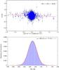 |
Fig. 2 NGC 1514: regression detection of a magnetic field on the second night, using uncontaminated stellar lines only. Methods R1 and RM yield a mean longitudinal magnetic field of ⟨Bz⟩ = −252 ± 85 G (top) and ⟨Bz⟩ = −252 ± 77 G (bottom), respectively. In the bottom panel, and the following figures of this kind, the histogram plot has a bin size of 5 G, and the (red) curve represents a Gaussian with the same mean value and standard deviation as the histogram data. |
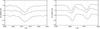 |
Fig. 3 IC 418: normalized Stokes I spectra of the central star in the spectral regions around the He ii line at λ 5411.5 Å (left) and the C iv lines λ 5801.3 and 5812.0 Å (right) obtained on three different nights. The spectra are shifted in vertical direction by 0.1 units for clarity, with the epoch increasing from bottom to top (the ordinate is correct for the lowermost spectrum). |
IC 418:
the central star of this young, elliptical planetary nebula was analyzed extensively (see, e.g., Mendez at al. 1988, 1992; Kudritzki et al. 1997; 2006; Pauldrach et al. 2004; Morisset & Georgiev 2009). The nebula is listed as a source of diffuse X-ray emission in Table 1 of Kastner et al. (2012). A more detailed recent analysis of the X-ray properties of IC 418 is listed in Ruiz et al. (2013). The projected rotational velocity of the central star was recently determined from a Fourier transform analysis of photospheric lines by Prinja et al. (2012), who found v sini = 56 km s-1.
Spectropolarimetric observations of the central star were carried out on three different nights. A significant spectral variability is detected in the He ii lines at λ 4541 and 5412 Å and in the C iv lines near λ 5800 Å. Note that these lines appear not to be blended with nebular emission lines (see also Fig. 1 of Mendez et al. 1988). In Fig. 3, we present as an example the variability of the He ii line at λ 5412 Å and of the C iv line profiles near λ 5800 Å.
A mean longitudinal magnetic field of negative polarity was detected at the 3σ level of significance on the second night when using the entire spectrum: ⟨Bz⟩ = −181 ± 54 G (method R1) and ⟨Bz⟩ = −177 ± 54 G (method RM), as shown in Fig. 4. The results obtained from both methods are essentially identical. However, when using the uncontaminated stellar lines only, the formal error increases to σB ≈ 100 G, and we are left with a 2σ signal in this case. It is noteworthy that all measurements for this object fall in the narrow range 175 ± 30 G. Nevertheless, adopting 100 G as the valid error estimate, the magnetic field detection in IC 418 must be considered as marginal and we infer a conservative 3σ upper limit for the mean longitudinal magnetic field of | ⟨Bz⟩ | ≲ 300 G.
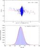 |
Fig. 4 IC 418: regression detection with method R1 of a ⟨Bz⟩ = −181 ± 54 G mean longitudinal magnetic field on the second night, using all lines (top). The corresponding ⟨Bz⟩ distribution obtained from method RM (bottom) deviates from a Gaussian (red curve) and indicates ⟨Bz⟩ = −177 ± 54 G. |
NGC 2346:
the optical spectrum of the central star of this bipolar PN is largely dominated by a companion of spectral type A5 V (e.g., De Marco 2009). The inspection of the Stokes I spectra obtained on three different nights indicates a very low spectral variability, as in the case of NGC 1514. Higher resolution spectra would be needed to establish a possible low-amplitude variability of the A-type stellar spectrum.
None of our spectropolarimetric measurements indicates the presence of a magnetic field signal. We conclude that the mean longitudinal magnetic field of the A-type companion, | ⟨Bz⟩ |, does not exceed 300 G.
According to Kastner et al. (2012), neither the central star (wind) nor the central cavity of the PN shows detectable X-ray emission.
NGC 2392:
the spectrum of the central star of this round/ elliptical PN was analyzed extensively (see, e.g., Mendez at al. 1988, 1992; Kudritzki et al. 1997; 2006; Pauldrach et al. 2004). According to Kastner et al. (2012), the central cavity of the nebula is a source of diffuse X-ray emission and, in addition, harbors a hard X-ray point source. A more detailed recent analysis of the X-ray properties of NGC 2392 is presented by Ruiz et al. (2013). Possibly, the central star has a late-type (dM) companion (Ciardullo et al. 1999).
No significant line profile variability is detected, neither in the Stokes I nor in the Stokes V spectra. Similarly, no significant magnetic field signal was detected on either observing night. Typical 1σ errors are ≈80 G when the entire spectrum is used, and ≈150 G when only the clean stellar lines are considered for the magnetic field measurement. A conservative 3σ upper limit for the mean longitudinal magnetic field of the central star of NGC 2392 is therefore | ⟨Bz⟩ | ≲ 450 G.
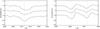 |
Fig. 5 Hen 2-108: normalized Stokes I spectra of the central star of the round planetary nebula in the spectral regions around the He ii line at λ 5411.5 Å (left) and the C iv doublet at λ 5801.3 and 5812.0 Å (right) obtained on three different nights. The spectra are shifted in vertical direction by 0.1 units for clarity, with the epoch increasing from bottom to top. |
Hen 2-36:
the optical spectrum of the central star of this bipolar PN is largely dominated by a companion of spectral type A. Spectral variability is very weak in both Stokes I and Stokes V spectra. Our measurements on two different observing nights show no evidence for the presence of a magnetic field in the central star of Hen 2-36, neither with method R1 nor with method RM, and irrespective of the considered spectral range. With typical errors of σB ≈ 100 G, we estimate a 3σ upper limit of | ⟨Bz⟩ | ≲ 300 G.
LSS 1362:
using spectropolarimetric data obtained with FORS 1, Jordan et al. (2005) reported the detection of a magnetic field of the order of several kG. Leone et al. (2011; 2014) reobserved the central star with FORS 2 but, similar to the case of NGC 1360, the authors could not confirm the presence of a magnetic field within an uncertainty of ~290 G. Likewise, Jordan et al. (2012) reanalyzed their own data and concluded that no magnetic field is detectable in this star. As with NGC 1360, our observations with FORS 2 on two different nights, with an uncertainty of about 300 G, do not indicate the presence of a magnetic field, in full agreement with these two recent works. A conservative 3σ upper limit for the mean longitudinal field of this central star is estimated to be | ⟨Bz⟩ | ≲ 800 G.
NGC 3132:
the optical spectrum of the central star of this elliptical PN is largely dominated by a companion of spectral type A2 IV-V (e.g., De Marco 2009). The inspection of the Stokes I spectra obtained on two different nights indicates a very low spectral variability, as in the other targets with A-type companions.
No significant (≳3σ for both sets of lines) mean longitudinal magnetic field was measured on either night, even though the error estimates of both methods (R1 and RM) are less than 100 G. The estimated 3σ upper limit for the mean longitudinal magnetic field of the A star companion is therefore relatively low, | ⟨Bz⟩ | ≲ 270 G.
No X-ray detection is reported for NGC 3132 by Kastner et al. (2012), neither from the planetary nebula nor from its central star.
Hen 2-108:
the spectrum of the central star of this round PN appears very similar to that of IC 418 (cf. Fig. 1, and Fig. 1 of Mendez et al. 1988). According to Tylenda et al. (1993), the central star of Hen 2-108 is a weak emission line star. Such stars have normal chemical composition, but show narrow lines from the λ 4650 N iii–C iii–C iv blend and the C iv λ 5806 doublet; C iii λ 5696 is absent or weak, while He ii λ 4686 emission is often seen. These lines are also seen in some massive O-type stars, low-mass X-ray binaries, and cataclysmic variables. Further analyses of the central star can be found in Mendez et al. (1988; 1992) and Pauldrach et al. (2004). No information is available concerning the X-ray emission of this PN.
The Stokes I spectra show some variability, as demonstrated in Fig. 5, where we display the variable stellar line profiles of He ii λ 5412 Å and the C iv lines near λ 5800 Å. However, we do not detect any mean longitudinal magnetic field at a significance level of 3σ on any of the three nights, irrespective of the adopted method and set of lines. Accepting the larger error estimates derived with the restricted wavelength set star, we obtain a conservative 3σ upper limit for the mean longitudinal field of this central star of | ⟨Bz⟩ | ≲ 700 G.
Hen 2-113:
the central star of this bipolar PN is H-deficient, classified as a Wolf-Rayet star of type [WC11] (Mendez & Niemela 1977; Tylenda et al. 1993). Hen 2-113 was not yet observed by Chandra, and no other information is available concerning the X-ray emission of this PN.
The target Hen 2-113, with a rich emission line spectrum, shows a variable slope of the continuum in Stokes V spectra obtained at different epochs. Such variable continuum slopes were previously detected in our measurements of a few Herbig Ae stars with complex circumstellar environment, a few WR stars, and in the magnetic Of?p star HD 148937, which is surrounded by the circumstellar nebula NGC 6164-65 that expands with a projected velocity of about 30 km s-1 (Leitherer & Chavarria 1987). The Stokes V spectra for Hen 2-113 were rectified before the magnetic field measurements were made.
A weak, but significant mean longitudinal magnetic field of negative polarity was detected with both method R1 and RM on the first observing night: ⟨Bz⟩ = −58 ± 18 G and ⟨Bz⟩ = −58 ± 24 G, respectively, when using the entire spectrum (wavelength set all), and ⟨Bz⟩ = −78 ± 25 G and ⟨Bz⟩ = −80 ± 26 G, respectively, when using the clean stellar lines only (wavelength set star). The latter detection is illustrated in the top panel of Fig. 6. Note that the formal error of the linear regression is particularly small in this case, mainly because the spread of the data points in x is large (cf. Eq. (B.4)) due to the presence of sharp emission lines (large dI/ dλ). As before, methods R1 and RM provide essentially the same error estimates, suggesting that the detection is solid.
In the case of Hen 2-113, we have derived another independent error estimate based on an experiment with simulated data (see Appendix C). This experiment shows that, under somewhat idealized conditions, our analysis method is expected to have a typical 1σ error of about 35 G, given the spectral resolution and signal-to-noise ratio of the present observations. This error estimate is somewhat larger than those reported above from methods R1 and RM. We speculate that this mismatch may be related to the fact that the number of lines in the synthetic spectrum is lower than in the observed spectrum. Nevertheless, the numerical experiment with synthetic spectra indicates that the errors obtained from the actual measurements in the range σB = 18 to 30 G are not unrealistic, and that the 3σ detection limit of our present measurements of Hen 2-113 is as low as | ⟨Bz⟩ | ≈ 120 G.
Hen 2-131:
according to Tylenda et al. (1993) the central star is a weak emission line star. No information is available concerning the X-ray emission of this elliptical planetary nebula.
The Stokes I spectra appear to be variable. In Fig. 7 we present as an example the C iii λ 4650.2 line profile variability detected in the Stokes I spectra obtained on both observing nights.
Relying on method R1, and using the entire spectrum, a weak mean longitudinal magnetic field was detected on both observing nights at a formal significance level of ≳3σ: ⟨Bz⟩ = −92 ± 29 G and ⟨Bz⟩ = −120 ± 32 G, on the first and second night, respectively. The latter detection is illustrated in Fig. 8 (top). Relying instead on method RM, we obtain very similar magnetic field strengths, but slightly larger error bars: ⟨Bz⟩ = −90 ± 41 G and ⟨Bz⟩ = −119 ± 50 G (Fig. 8, bottom). Similar results are derived when using the clean stellar lines only, again indicating a mean longitudinal magnetic field of ≈−100 G, but only with a significance of 2σ. Hen 2-131 may thus be a marginal detection.
The 3σ upper limit for the mean longitudinal field of this central star is as low as | ⟨Bz⟩ | ≲ 150 G.
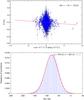 |
Fig. 6 Hen 2-113: regression detection of a ⟨Bz⟩ = −78 ± 25 G mean longitudinal magnetic field on the first night with method R1, using uncontaminated stellar lines only (top), and corresponding (slightly non-Gaussian) distribution of ⟨Bz⟩ obtained from method RM (bottom). |
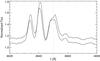 |
Fig. 7 Hen 2-131: normalized Stokes I spectra of the central star in the spectral region around the C iii feature at λ 4650.2 Å, obtained on two different nights. The spectrum of the second night is shifted upward in vertical direction by 0.1 units for clarity. |
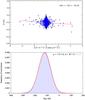 |
Fig. 8 Hen 2-131: regression detection of a ⟨Bz⟩ = −120 ± 32 G mean longitudinal magnetic field with method R1, using the entire spectrum (top), and corresponding distribution of ⟨Bz⟩ derived from method RM (bottom). |
4. Discussion
4.1. Significance of our magnetic field measurements
Most of the stars of our sample were not studied at the achieved accuracy before, and the present study allows us to put further constraints on the strength of the magnetic fields in central stars of planetary nebulae. In Fig. 9 we present a synopsis of the results of our magnetic field measurements based on the entire spectrum (top) and on clean stellar lines only (bottom).
The achievable measurement accuracy is limited by the comparatively low number of useful spectral lines for the magnetic field diagnostics in the central stars of planetary nebulae. In addition, since no linear polarization measurements exist for our sample stars, it is difficult to assess how our detections are affected by crosstalk. It is therefore challenging to provide reliable estimates for ⟨Bz⟩.
In addition to the formal errors from the linear regression (method R1, Appendix B.1), we have alternatively considered an independent error estimate obtained from a bootstrapping analysis (method RM, Appendix B.2). As may be seen from Fig. 9, the errors from method RM turn out to be surprisingly similar to those from method R1. This close agreement suggests that our error estimates can be considered realistic.
If we require that a detection is only valid if it is found with both method R1 and method RM when using the wavelength set star (clean stellar lines only), then we count two 3σ detections, namely NGC 1514 (second night) and Hen 2-113 (first night), and two cases where our measurements indicate a magnetic field at the 2σ significance level, namely IC 418 (second night) and Hen 2-131 (first night). IC 418 is, in fact, a 3σ detection with wavelength set all. For the two emission line objects Hen 2-113 and Hen 2-131, the formal error is remarkably small, in the case of Hen 2-113 even smaller than the theoretical estimate derived from numerical experiments with synthetic spectra (Appendix C), and hence these formal detections must be considered with some caution.
In all cases, the magnetic field is detected only during one out of two useful observing nights, which, in view of the expected rotation periods of only a few days, might be attributed to rotational modulation by large-scale magnetic structures.
In summary, we cannot claim a clear positive detection of a magnetic field in any of the PN central stars of our sample. What we can do, though, is to estimate individual upper limits of | ⟨Bz⟩ |, as set by the quality of our measurements and the sensitivity of our analysis method (see Table 3, Col. 9). In the following, we investigate whether such upper limits are sufficient to rule out the PN magnetic shaping scenario.
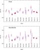 |
Fig. 9 Summary of our magnetic field measurements for the 12 targets of our sample, using wavelength set all (entire spectrum, top) and wavelength set star (clean stellar lines only, bottom) as listed in Table 2. Open symbols indicate non-detections, small and large filled dots (red) stand for 2σ and 3σ detections, respectively, with method R1, while (blue) stars mark 2σ (4 rays) and 3σ (8 rays) detections with method RM. Error bars refer to 1σ errors from method R1 (red) and RM (blue), respectively. |
Physical parameters of the central stars of the PNe observed in the present program (excluding those whose spectra are outshone by an A-type companion).
4.2. The magnetized stellar wind
If large-scale (dipole-like) magnetic fields are present at the surface of a central star, they are carried along with the fast stellar wind and are wound up due to stellar rotation. At large distances from the star, the field is essentially toroidal (i.e. has only an azimuthal component). The impact of the magnetic field on the shaping of the shocked wind and the inner nebula is described by the magnetization parameter σM, the ratio of magnetic to kinetic energy density of the magnetized stellar wind (see, e.g., Chevalier & Luo 1994): 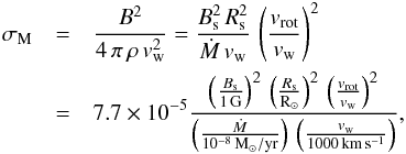 (3)where Bs is the magnetic field at the stellar surface, Rs the stellar radius, and Ṁ and vw the mass loss rate and the terminal velocity of the central star’s fast wind. Theoretical considerations show that significant deviation from spherical nebular expansion requires a minimum magnetization of the stellar wind given by σM ≳ 10-4 (Chevalier & Luo 1994). While the wind is essentially unaffected by the magnetic field at such low values of σM, the magnetic pressure becomes significant inside the hot bubble of shocked gas, thus allowing for magnetic shaping of the nebula (see Sect. 4.3).
The condition σM ≳ 10-4 can be expressed as 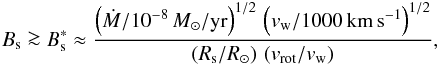 (4)where
  is in units of Gauss.
We compiled the relevant physical parameters of our program stars in Table 3 (except for the four objects whose spectra are dominated by an A-type companion), allowing us to estimate according to Eq. (4), assuming vrot ≈ v sin i, or vrot ≈ 10 km s-1 where no measurement of v sin i is available. For most of the central stars of our sample, turns out to be weaker than 100 G (see Table 3). Note that for the central stars of IC 418 and NGC 2392, is particularly low because of the high rotational velocity and the low wind speed, respectively.
Assuming that any potential large-scale magnetic field at the surface of the central stars would be dipole-like, we make the statistical approximation Bs ≈ 3 ⟨Bz⟩. The upper limit of Bs derived from out measurements, | 3 ⟨Bz⟩ |, is listed individually for each target in Table 3 (Col. 9).
We find that, except for two of our targets (NGC 246 and LSS 1362), the upper limit for ⟨Bz⟩ that excludes magnetic shaping lies at least a factor of 10 below the upper limit provided by our measurements. For most of our targets, we therefore cannot rule out the presence of a stellar surface magnetic field that is strong enough for shaping the present fast wind of the central stars.
We have to keep in mind, however, that the shaping of the PN must have occurred during a preceeding period of time, starting in the early stages of post-AGB evolution. We are therefore interested to know whether the magnetic field was strong enough to influence the stellar wind when the nebula was just about to form. For this purpose, we extrapolate Bs backward in time, starting at the current value, and assuming that (i) the stellar luminosity is constant,  = const.; (ii) the angular momentum of the star is conserved, vrotRs = const.; (iii) the fast wind velocity scales with the escape velocity,
  = const.; (iv) Ṁ = const.; and (v) the total magnetic flux is conserved,
  = const., implying that σM increases strongly during the time evolution as
  .
.
To ensure that the magnetization parameter σM exceeds the critical value of 10-4 already at an earlier time, t = t0, the magnetic field strength at the current time, t = t1, must fulfill the condition 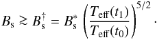 (5)In Table 3, we also provide the value of for the assumption Teff(t0) = 20 kK. We see that clearly exceeds the upper limit for the measured stellar field strength, Bs ≈ 3 ⟨Bz⟩, in the case of NGC 246 and LSS 1362, indicating that magnetic shaping is not expected to play any role for these two round/elliptical objects. On the other hand, we find that the upper limit for Bs estimated from our magnetic field measurements is still about a factor of 5 to 10 higher than for the five PNe IC 418, NGC 2392, Hen 2-108, Hen 2-113, and Hen 2-131. For these objects, our measurements do not rule out the possibility that their nebulae have been subject to magnetic shaping since early on in their post-AGB evolution when Teff ≈ 20 kK, or even since shortly after the end of the AGB evolution (see below). The situation in less clear for NGC 1360 where is intermediate between the two extremes mentioned above.
The estimation of the magnetization parameter at even earlier times, near the tip of the AGB (t = tAGB, Teff ≈ 5 kK), is more uncertain because the above assumption of constant mass loss rate is no longer valid below Teff ≈ 20 kK (t<t0). Assuming instead that Ṁ decreases by a factor of 100 between t = tAGB and t = t0, while at the same time vw increases by a factor of 100, we find that, roughly, σM(tAGB) /σM(t0) ≈ 0.1, in agreement with the numbers quoted by García-Segura et al. (1999) based on Reid at al. (1979). We conclude that the slow but massive AGB wind is probably unaffected by magnetic shaping as long as , which is the case for most of our targets. For only two targets, IC 418, and NGC 2392, our measurements do not even rule out a marginal magnetic influence on the very early post-AGB wind.
4.3. Magnetic shaping of the hot bubble
The free wind of the central star is bounded by a strong reverse shock at radius R1 where the kinetic energy of the wind is thermalized. The shocked wind fills the so-called hot bubble, bounded by the contact discontinuity at outer radius R2. The strength of the magnetic field in the immediate pre-shock region, Bp, may be estimated from the stellar surface magnetic field, Bs, as Bp ~ Bs × vrot/vw × Rs/R1 (e.g., Chevalier & Luo 1994), where vrot and vw are the (equatorial) rotation velocity of the central star and the outflow velocity of its fast wind, while Rs and R1 is the radius of the central star and the inner radius of the hot bubble, respectively. Assuming R1 = 0.01 pc, we evaluated the ratio Bp/Bs for the central stars of our target list. The ratio lies in the range 1.7 × 10⁻⁹ to 3.5 × 10⁻⁷. We thus conclude that the strength of magnetic fields in the pre-shock region cannot exceed a few hundred μG. Such fields are too weak to influence the structure of the strong wind shock, however, according to the Chevalier & Luo (1994) model, the magnetic field builds up downstream as a consequence of the compressive flow inside the hot bubble.
The structure of the magnetized hot bubble is illustrated in Fig. 1 of Chevalier (1992) for the quasi-spherical case, assuming σM = 0.001, which is readily applicable to the shocked wind bubbles of PNe. Across the shock, B jumps from the pre-shock value Bp to a post-shock value of BX(R1) ≈ 16 × Bp. Because of the negative velocity gradient inside the hot bubble, the magnetic flux density increases outwards and rises to BX(R2) ≈ 320 × Bp at the outer edge of the hot bubble, assuming that R2 ≈ 5 × R1.
For sufficiently large σM, the magnetic field has a direct dynamical effect on the expansion of the hot bubble. Figure 1 of Chevalier (1992) shows that the magnetic pressure,  , can even exceed the thermal gas pressure, nekT, in the outer parts of large (old) bubbles. At the same time, the magnetic tension gives rise to a non-spherical expansion by reducing the driving force in the equatorial direction, thus leading to an elongated shape in the polar direction. This mechanism is at the heart of the magnetic shaping scenario.
According to the model assumptions made above in Sect. 4.2, the hot bubble of older nebulae are expected to harbor stronger magnetic fields than younger nebulae. For constant R1, we find that Bp increases as  . Since Teff typically increases by a factor of 10 during the post-AGB evolution, Bp would increase roughly by a factor of 1000. Taking into account that at the same time the central cavity expands by roughly a factor of 5 (see, e.g., Fig. 5 of Schönberner et al. 2005), we estimate that Bp is about 200 times larger in old compared to young PNe.
4.4. X-ray emission
According to the order of magnitude estimates given in Sect. 4.3, we may assume, as an upper limit, that the magnetic field varies in the X-ray emitting hot bubble between a few mG near the inner shock up to 100 mG strength near the outer contact discontinuity. Weak magnetic fields of this order of magnitude can easily suppress thermal conduction in the direction perpendicular to their field lines. According to Spitzer (1962), the factor by which the thermal conductivity is reduced in this direction with respect to the conductivity along the field lines (or the field-free case) can be expressed for a pure hydrogen plasma as 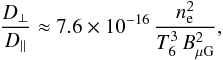 (6)where ne is the electron density in [cm-3], T6 the electron temperature in [106 K], and BμG the magnetic flux density in units of [10-6 G] (see also Balbus 1986). In the X-ray emitting cavity (ne ≈ 10, T6 ≳ 10, BμG ≳ 1) we obtain D⊥/D∥ ≲ 10-13, indicating that any thermal conduction perpendicular to the magnetic field lines is expected to be very effectively suppressed, even for field strengths that are many orders of magnitude below 1μG.
If the magnetic field has a purely toroidal orientation in the X-ray emitting central cavity, thermal conduction in the radial direction should be completely suppressed, even if the field is much weaker than those deduced in our present study. As a consequence, the luminosity of the diffuse X-ray emission should be significantly lower, and the characteristic X-ray temperature should be significantly higher than what is typically found in X-ray observations (see, e.g., Steffen et al. 2008). This dilemma may indicate that the nebular field geometry is different from purely toroidal. Alternatively, other physical mechanisms, such as turbulent mixing due to hydrodynamic instabilities at the contact discontinuity (e.g., Stute & Sahai 2006; Toala & Arthur 2014), may provide an efficient channel for radial heat exchange.
4.5. Central star magnetic field and nebular morphology
Two out of the three bipolar nebulae of our sample harbor a central star with an A-type binary companion (NGC 2346 and Hen 2-36). In these cases, the magnetic field measurement of the central stars proper is impossible due to contamination of their spectrum by the A-type companion. For the central star of the remaining bipolar PN, Hen 2-113, our magnetic field measurements provide marginal support for a magnetic origin of the bipolar nebular structure.
For the central star of the elliptical PN LSS 1362, our analysis showed that magnetic shaping is expected to be unlikely and is at best restricted to the present evolutionary stage. This might indicate that the elliptical shape of LSS 1362 has a non-magnetic background, but the constraints are weak. For the remaining six elliptical PNe, the magnetic shaping hypothesis cannot be constrained by our magnetic field estimates.
The only case where we can rule out significant magnetic shaping is NGC 246. Since this PN is indeed round, there is no reason here to invoke a non-magnetic shaping mechanism. No constraints can be derived for the other round PN, Hen 2-108.
In view of the poor statistics, it is clearly impossible to establish any firm empirical relation between the strength of the central star’s magnetic field and the morphological type of the associated planetary nebula. Given the rather low measurement accuracy, we also cannot find any clear inconsistencies that would invalidate the magnetic shaping hypothesis.
4.6. Central star magnetic field and X-ray emission
According to Sect. 4.4, both weak and strong magnetic fields suppress thermal conduction with essentially the same efficiency. From this perspective, we would not expect any correlation between the strength of the stellar magnetic field and the luminosity in diffuse X-rays. However, the thermal structure and density profile of the hot bubble can be significantly altered by the presence of sufficiently strong magnetic fields (cf. Sect. 4.3). Obviously, an empirical verification of a possible relation between stellar magnetic field strength and diffuse X-ray emission is impossible with our sample: only two of the elliptical nebulae show diffuse X-ray emission (IC 418 and NGC 2392) and in both cases only a (rather high) upper limit for the stellar magnetic field could be deduced.
On the other hand, the same two objects suggest that the presence of a central point source of hard X-ray emission is not related to the strength of the stellar magnetic field either. Our measurements indicate that the stellar magnetic field is unlikely to be significantly stronger in NGC 2392 than in IC 418, and yet NGC 2392 harbors an X-ray point source while IC 418 does not, which seems difficult to reconcile with the idea of a magnetic origin of the hard X-ray emission.
5. Conclusions
We have analyzed spectropolarimetric observations of 12 central stars of planetary nebulae carried out at the European Southern Observatory with FORS 2 mounted on the 8 m Antu telescope of the VLT. We find marginal evidence for weak mean longitudinal magnetic fields of about 200 G in the central star of the young elliptical nebula IC 418, and for even weaker magnetic fields of about 100 G in the emission-line spectra of the Wolf-Rayet type central star Hen 2-113 and the weak emission line star Hen 2-131. In general, however, we can only estimate upper limits for the mean longitudinal magnetic fields | ⟨Bz⟩ | in the range 120 to 800 G. We conclude that strong magnetic fields exceeding 1 kG are not widespread among PNe central stars.
Some of the observed central stars, including IC 418 and Hen 2-131, show a significant night-to-night spectrum variability of the stellar line profiles, which may be attributed to rotational modulation due to magnetic features or inhomogeneities in the stellar wind. Follow-up monitoring of these targets may be worthwhile to confirm the rotational/magnetic variability and to determine the related timescales.
Interestingly, the hypothesis that planetary nebulae are shaped by magnetic fields is not ruled out by our measurements. Theoretical order of magnitude estimates suggest that even weak magnetic fields well below the detection limit of our measurements are sufficient to contribute to the shaping of the surrounding nebulae throughout their evolution. We have to conclude that, at the present accuracy, the available measurements of central star magnetic fields can neither support nor rule out the magnetic shaping hypothesis for most of our targets. We can only infer for NGC 246 and LSS 1362 that magnetic shaping is not playing any significant role.
The only clear 3σ detection of a 250 G mean longitudinal field is achieved for the A-type companion of the central star of NGC 1514. Even though the mass loss of an A-type star is negligible compared to that of the true central star, the magnetic field of the A-type companion might interact with the wind of the central star. Whether or not such interaction would play any role in shaping the surrounding planetary nebula is unclear. In any case, we can assume that both stars formed and evolved in a common environment. The presence of a magnetic field in the companion of the central star is of great interest in the context of understanding the origin of magnetic fields in A-type stars, since only a few magnetic Ap stars are known to belong to close binary systems.
Acknowledgments
C.S. was supported by funds of DFG (project SCHO394/ 29-1) and Land Brandenburg (SAW funds from WGL), and also by funds of PTDESY-05A12BA1. We thank Martin Wendt for fruitful discussions of statistical methods, and the referee, John Landstreet, for constructive criticism that led to significant improvement of this paper.
References
- Bagnulo, S., Landstreet, J. D., Fossati, L., & Kochukhov, O. 2012, A&A, 538, A129 [NASA ADS] [CrossRef] [EDP Sciences] [Google Scholar]
- Balbus, S. A. 1986, ApJ, 304, 787 [NASA ADS] [CrossRef] [Google Scholar]
- Balick, B., & Frank, A. 2002, ARA&A, 40, 439 [NASA ADS] [CrossRef] [Google Scholar]
- Blackman, E. G. 2009, in IAU Symp. 259, eds. K. G. Strassmeier, & A. G. Kosovichev, J. E. Beckman, 35 [Google Scholar]
- Bond, H. E., & Ciardullo, R. 1999, PASP, 111, 217 [NASA ADS] [CrossRef] [Google Scholar]
- Chevalier, R. A. 1992, ApJ, 397, L39 [NASA ADS] [CrossRef] [Google Scholar]
- Chevalier, R. A., & Luo, D. 1994, ApJ, 421, 225 [NASA ADS] [CrossRef] [Google Scholar]
- Ciardullo, R., Bond, H. E., Sipior, M. S., et al. 1999, AJ, 118, 488 [NASA ADS] [CrossRef] [Google Scholar]
- Corradi, R. L. M., & Schwarz, H. E. 1995, A&A, 293, 871 [NASA ADS] [Google Scholar]
- De Marco, O. 2009, PASP, 121, 316 [NASA ADS] [CrossRef] [Google Scholar]
- De Marco, O., & Crowther, P. A. 1998, MNRAS, 296, 419 [NASA ADS] [CrossRef] [Google Scholar]
- Douchin, D., De, M. O., Jacoby, G. H., et al. 2012, in SF2A-2012: Proc. of the Annual meeting of the French Society of Astronomy and Astrophysics, eds. S. Boissier, P. de Laverny, N. Nardetto, R. Samadi, D. Valls-Gabaud, & H. Wozniak, 325 [Google Scholar]
- Drilling, J. S. 1983, ApJ, 270, L13 [NASA ADS] [CrossRef] [Google Scholar]
- García-Díaz, M. T., López, J. A., García-Segura, G., et al. 2008, ApJ, 676, 402 [NASA ADS] [CrossRef] [Google Scholar]
- García-Segura, G., Langer, N., Różyczka, M., & Franco, J. 1999, ApJ, 517, 767 [NASA ADS] [CrossRef] [Google Scholar]
- Gräfener, G., Koesterke, L., & Hamann, W.-R. 2002, A&A, 387, 244 [NASA ADS] [CrossRef] [EDP Sciences] [Google Scholar]
- Hamann, W.-R., & Gräfener, G. 2003, A&A, 410, 993 [NASA ADS] [CrossRef] [EDP Sciences] [Google Scholar]
- Heap, S. R. 1977, ApJ, 215, 609 [NASA ADS] [CrossRef] [Google Scholar]
- Herald, J. E., & Bianchi, L. 2011, MNRAS, 417, 2440 [NASA ADS] [CrossRef] [Google Scholar]
- Hoogerwerf, R., Szentgyorgyi, A., Raymond, J., et al. 2007, ApJ, 670, 442 [NASA ADS] [CrossRef] [Google Scholar]
- Hubrig, S., Kurtz, D. W., Bagnulo, S., et al. 2004a, A&A, 415, 661 [NASA ADS] [CrossRef] [EDP Sciences] [Google Scholar]
- Hubrig, S., Szeifert, T., Schöller, M., et al. 2004b, A&A, 415, 685 [NASA ADS] [CrossRef] [EDP Sciences] [Google Scholar]
- Hubrig, S., Schöller, M., & Kholtygin, A. F. 2014, MNRAS, 440, 1779 [NASA ADS] [CrossRef] [Google Scholar]
- Jordan, S., Werner, K., & O’Toole, S. J. 2005, A&A, 432, 273 [NASA ADS] [CrossRef] [EDP Sciences] [Google Scholar]
- Jordan, S., Bagnulo, S., Werner, K., & O’Toole, S. J. 2012, A&A, 542, A64 [NASA ADS] [CrossRef] [EDP Sciences] [Google Scholar]
- Kastner, J. H., Montez, Jr., R., Balick, B., et al. 2012, AJ, 144, 58 [NASA ADS] [CrossRef] [EDP Sciences] [Google Scholar]
- Koesterke, L., Dreizler, S., & Rauch, T. 1998, A&A, 330, 1041 [NASA ADS] [Google Scholar]
- Kudritzki, R.P., Mendez, R. H., Puls, J., & McCarthy, J. K. 1997, Planetary Nebulae, IAU Symp., 180, 64 [NASA ADS] [Google Scholar]
- Kudritzki, R. P., Urbaneja, M. A., & Puls, J. 2006, Planetary Nebulae in our Galaxy and Beyond, IAU Proc., 234, 119 [Google Scholar]
- Lagadec, E., Chesneau, O., Matsuura, M., et al. 2006, A&A, 448, 203 [NASA ADS] [CrossRef] [EDP Sciences] [Google Scholar]
- Leitherer, C., & Chavarria-K., C. 1987, A&A, 175, 208 [NASA ADS] [Google Scholar]
- Leone, F., Martínez González, M. J., Corradi, R. L. M., et al. 2011, ApJ, 731, L33 [NASA ADS] [CrossRef] [Google Scholar]
- Leone, F., Corradi, R. L. M., Martínez González, M. J., Asensio Ramos, A., & Manso Sainz, R. 2014, A&A, 563, A43 [NASA ADS] [CrossRef] [EDP Sciences] [Google Scholar]
- Marten, H., & Schönberner, D. 1991, A&A, 248, 590 [Google Scholar]
- Mellema, G. 1994, A&A, 290, 915 [NASA ADS] [Google Scholar]
- Mellema, G. 1995, MNRAS, 277, 173 [NASA ADS] [Google Scholar]
- Mellema, G. 1997, A&A, 321, L29 [NASA ADS] [Google Scholar]
- Mendez, R. H., & Niemela, V. S. 1977, MNRAS, 178, 409 [Google Scholar]
- Mendez, R. H., Kudritzki, R. P., Herrero, A., Husfeld, D., & Groth, H. G. 1988, A&A, 190, 113 [NASA ADS] [Google Scholar]
- Mendez, R. H., Kudritzki, R. P., & Herrero, A. 1992, A&A, 260, 329 [NASA ADS] [Google Scholar]
- Morisset, C., & Georgiev, L. 2009, A&A, 507, 1517 [NASA ADS] [CrossRef] [EDP Sciences] [Google Scholar]
- Pauldrach, A. W. A., Hoffmann, T. L., & Méndez, R. H. 2004, A&A, 419, 1111 [NASA ADS] [CrossRef] [EDP Sciences] [Google Scholar]
- Perinotto, M., Schönberner, D., Steffen, M., & Calonaci, C. 2004, A&A, 414, 993 [NASA ADS] [CrossRef] [EDP Sciences] [Google Scholar]
- Phillips, J. P. 2003, MNRAS, 344, 501 [NASA ADS] [CrossRef] [Google Scholar]
- Press W. H., Teukolsky S. A., Vetterling W. T., & Flannery B. P. 2007, 3rd edn. (Cambridge: University Press), 780 [Google Scholar]
- Prinja, R. K., Massa, D. L., Urbaneja, M. A., & Kudritzki, R.-P. 2012, MNRAS, 422, 3142 [NASA ADS] [CrossRef] [Google Scholar]
- Rauch, T., Koeper, S., Dreizler, S., et al. 2003, IAU Symp. 215, eds. A. Maeder, & P. R. J. Eenens, ASP, 573 [Google Scholar]
- Reid, M. J., Moran, J. M., Leach, R. W., et al. 1979, ApJ, 227, L89 [NASA ADS] [CrossRef] [Google Scholar]
- Rivinius, T., Szeifert, T., Barrera, L., et al. 2010, MNRAS, 405, L46 [NASA ADS] [CrossRef] [Google Scholar]
- Ruiz, N., Chu, Y. H., Gruendl, R. A., et al. 2013, ApJ, 767, 35 [NASA ADS] [CrossRef] [Google Scholar]
- Schönberner, D., Jacob, R., & Steffen, M. 2005, A&A, 441, 573 [NASA ADS] [CrossRef] [EDP Sciences] [Google Scholar]
- Soker, N. 2006, PASP, 118, 260 [NASA ADS] [CrossRef] [Google Scholar]
- Spitzer, L. 1962, Physics of Fully Ionized Gases, 2nd edn. (New York: Interscience) [Google Scholar]
- Steffen, M., & Schönberner, D. 2006, Planetary Nebulae in our Galaxy and Beyond, IAU Symp., 234, 285 [NASA ADS] [CrossRef] [Google Scholar]
- Steffen, M., Schönberner, D., & Warmuth, A. 2008, A&A, 489, 173 [NASA ADS] [CrossRef] [EDP Sciences] [Google Scholar]
- Stute, M., & Sahai, R. 2006, ApJ, 651, 882 [NASA ADS] [CrossRef] [Google Scholar]
- Toala, J. A., & Arthur, S. J. 2014, MNRAS, 443, 3486 [NASA ADS] [CrossRef] [Google Scholar]
- Traulsen, I., Hoffmann, A. I. D., Rauch, T., et al. 2005, 14th European Workshop on White Dwarfs, ASP Conf. Ser., 334, 325 [NASA ADS] [Google Scholar]
- Tylenda, R., Acker, A., & Stenholm, B. 1993, A&AS, 102, 595 [NASA ADS] [Google Scholar]
- Villaver, E., Manchado, A., & García-Segura, G. 2002, ApJ, 581, 1204 [NASA ADS] [CrossRef] [Google Scholar]
- Werner, K., & Herwig, F. 2006, PASP, 118, 183 [NASA ADS] [CrossRef] [Google Scholar]
Appendix A: Selected wavelength regions
Wavelength region all:
comprises the entire spectral range, but excludes the nebular [O iii] emission lines near 5000 Å and pixels affected by instrumental artifacts, as identified in the null spectra and removed by 3σ clipping. For each object, the spectra shown in Fig. A.1 are plotted over the useful spectral range defined in this way (referred to as wavelength set all in this work).
Wavelength region star:
is obtained from wavelength region all by excluding additional spectral windows that contain nebular emission lines. The latter could be identified in the original CCD frames in traces located above and below the spectrum of the central star. The spectral regions excluded in this procedure are indicted as horizontal bars 0.2 units below the respective stellar continuum of each object in Fig. A.1.
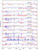 |
Fig. A.1 Normalized FORS 2 Stokes I spectra of the 12 central stars in our sample, displayed with a vertical offset of 1 unit between adjacent spectra. For each object, the displayed spectra (blue) define wavelength set all (entire spectrum), gaps indicating the excluded regions, while wavelength set star (clean stellar lines only) is obtained by excluding the regions marked by the (red) horizontal bars 0.2 units below the respective stellar continuum. |
Appendix B: Deriving ⟨Bz⟩ and σB from linear regression
The mean longitudinal magnetic field ⟨Bz⟩ is derived from the fundamental relation 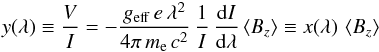 (B.1)(cf. Eq. (2) and related text for the definition of the different symbols). For the present analysis, we use the original wavelength scale provided by our pipeline (Δλ = 0.75 Å), avoiding interpolation to finer wavelength steps.
Appendix B.1: Method R1
Given the original dataset {xi(λ),yi(λ)}i = 1,N, where N is the total number of considered spectral bins, and assuming that relation (B.1) is valid both for absorption and emission lines, with geff ≈ 1.2, we compute ⟨Bz⟩ from linear regression (e.g., Press et al. 2007) as: 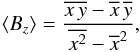 (B.2)where we have defined
 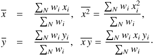 (B.3)The weight of each pixel is given by the square of the signal-to-noise ratio of Stokes V,
  . Considering the propagation of errors, assuming that the errors in x are negligible, we obtain the formal 1 σ uncertainty of ⟨Bz⟩ as
 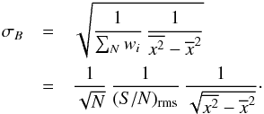 (B.4)As a sanity check, we also compute the quantity
 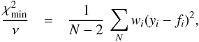 (B.5)where fi is the value obtained from the best fitting straight line,
 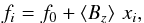 (B.6)with
 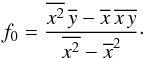 (B.7)Whenever
  , σB is multiplied by the factor
  to obtain the final error estimate of ⟨Bz⟩. In general, this factor is ≲1, and never exceeds 1.07 for the applications considered in this paper.
Appendix B.2: Method RM
In this Monte-Carlo type approach, we generate M = 106 statistical variations of the original dataset {xi(λ),yi(λ)}i = 1,N by bootstrapping (e.g., Rivinius et al. 2010). Each of the M artificial datasets comprises N data points, obtained by randomly drawing N times a data point from the original sample, assigning the same probability of being drawn to all data points. For each of these M generated datasets, we derive the value ⟨Bz⟩m using Eq. (B.2), taking the weights wi of the individual data points into account. The expectation value of ⟨Bz⟩ is given by the mean of the distribution, 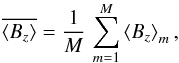 (B.8)and the 1σ error is estimated from the standard deviation of the distribution, even if the latter is not necessarily Gaussian:
  (B.9)In this scheme, outliers in the original dataset will automatically translate into an increased error estimate, even if the formal error (
 ) assigned to such data points is small.
Appendix C: Error of ⟨Bz⟩ from simulated data
Yet another independent estimate of the error margin of our magnetic field measurements is obtained from the following test based on simulated data. Among our targets, we select the [WC]-type central star Hen2-113. With the Potsdam Wolf-Rayet (PoWR) model atmosphere code (Gräfener et al. 2002; Hamann & Gräfener 2003) we calculate a synthetic spectrum that is similar to the observed spectrum of this star. We restrict the normalized synthetic spectrum to the observed wavelength range (4000–6000 Å), convolve it with a Gaussian of 3 Å according to the spectral resolution of FORS 2, and bin the data to the pixel size of 0.66 Å.
Then we add to the simulated spectrum artificial noise as a Gaussian distribution with a standard deviation equal to SN-1. The signal-to-noise ratio, SN, is set to 920. This corresponds to the quality of our Hen2-113 observations after all spectra from one night that belong to the same polarization channel have been coadded.
Two such simulated spectra with independent statistical noise are now taken to mimic the ordinary and the extra-ordinary polarization channel, respectively. These data are analyzed for their Zeeman shift in the same way as the real observations. The result is a “measured” field strength ⟨Bz⟩. The whole procedure is now repeated 1001 times with the same simulated data, but independent artificial noise. The distribution of the obtained field strength ⟨Bz⟩ is plotted as a histogram in Fig. C.1. The obtained ⟨Bz⟩ values scatter around zero with a mean deviation of 35 Gauss.
Summarizing, this test was based on the following assumptions: (1) the line spectrum is similar to our simulated, normalized spectrum for Hen2-113; (2) the observed spectra have a S/N of 920 per pixel in the ordinary as well as in the extra-ordinary channel; (3) statistical noise is the only source of errors; (4) both emission and absorption lines are included in the analysis and “feel” the same Zeeman splitting. Under these assumptions, the value obtained for ⟨Bz⟩ with FORS 2 via our method of analysis has a theoretical 1σ error of ≈35 Gauss. Note that this error is independent of the magnetic field strength assumed in modeling the simulated Stokes V spectrum (here ⟨Bz⟩ = 0).
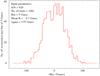 |
Fig. C.1 Distribution of 1001 ⟨Bz⟩ measurements on simulated data for Hen2-113 with input field ⟨Bz⟩ = 0 and artificial noise corresponding to S/N = 920 per pixel in each channel. As the results show, the method has in this case a 1σ error of 35 Gauss. |
This exercise suggests that the small formal 1σ error obtained from the actual measurements of Hen2-113 with methods R1 and RM in the range σB = 18 to 30 G is not unrealistic, though it may be somewhat underestimated. Note, however, that a number of lines seen in the observation are missing in the synthetic spectrum.
All Tables
List of PNe central stars observed in the framework of our program, ordered by increasing RA.
Physical parameters of the central stars of the PNe observed in the present program (excluding those whose spectra are outshone by an A-type companion).
All Figures
|
Fig. 1 Normalized FORS 2 Stokes I spectra of the 12 central stars in our sample, displayed with a vertical offset of 1 unit between adjacent spectra. The strongest spectral lines are identified. The forbidden [O iii] nebular emission lines close to 5000 Å are marked in green. They may appear in absorption (e.g., NGC 2392) due to imperfect background subtraction. |
| In the text | |
|
Fig. 2 NGC 1514: regression detection of a magnetic field on the second night, using uncontaminated stellar lines only. Methods R1 and RM yield a mean longitudinal magnetic field of ⟨Bz⟩ = −252 ± 85 G (top) and ⟨Bz⟩ = −252 ± 77 G (bottom), respectively. In the bottom panel, and the following figures of this kind, the histogram plot has a bin size of 5 G, and the (red) curve represents a Gaussian with the same mean value and standard deviation as the histogram data. |
| In the text | |
|
Fig. 3 IC 418: normalized Stokes I spectra of the central star in the spectral regions around the He ii line at λ 5411.5 Å (left) and the C iv lines λ 5801.3 and 5812.0 Å (right) obtained on three different nights. The spectra are shifted in vertical direction by 0.1 units for clarity, with the epoch increasing from bottom to top (the ordinate is correct for the lowermost spectrum). |
| In the text | |
|
Fig. 4 IC 418: regression detection with method R1 of a ⟨Bz⟩ = −181 ± 54 G mean longitudinal magnetic field on the second night, using all lines (top). The corresponding ⟨Bz⟩ distribution obtained from method RM (bottom) deviates from a Gaussian (red curve) and indicates ⟨Bz⟩ = −177 ± 54 G. |
| In the text | |
|
Fig. 5 Hen 2-108: normalized Stokes I spectra of the central star of the round planetary nebula in the spectral regions around the He ii line at λ 5411.5 Å (left) and the C iv doublet at λ 5801.3 and 5812.0 Å (right) obtained on three different nights. The spectra are shifted in vertical direction by 0.1 units for clarity, with the epoch increasing from bottom to top. |
| In the text | |
|
Fig. 6 Hen 2-113: regression detection of a ⟨Bz⟩ = −78 ± 25 G mean longitudinal magnetic field on the first night with method R1, using uncontaminated stellar lines only (top), and corresponding (slightly non-Gaussian) distribution of ⟨Bz⟩ obtained from method RM (bottom). |
| In the text | |
|
Fig. 7 Hen 2-131: normalized Stokes I spectra of the central star in the spectral region around the C iii feature at λ 4650.2 Å, obtained on two different nights. The spectrum of the second night is shifted upward in vertical direction by 0.1 units for clarity. |
| In the text | |
|
Fig. 8 Hen 2-131: regression detection of a ⟨Bz⟩ = −120 ± 32 G mean longitudinal magnetic field with method R1, using the entire spectrum (top), and corresponding distribution of ⟨Bz⟩ derived from method RM (bottom). |
| In the text | |
|
Fig. 9 Summary of our magnetic field measurements for the 12 targets of our sample, using wavelength set all (entire spectrum, top) and wavelength set star (clean stellar lines only, bottom) as listed in Table 2. Open symbols indicate non-detections, small and large filled dots (red) stand for 2σ and 3σ detections, respectively, with method R1, while (blue) stars mark 2σ (4 rays) and 3σ (8 rays) detections with method RM. Error bars refer to 1σ errors from method R1 (red) and RM (blue), respectively. |
| In the text | |
|
Fig. A.1 Normalized FORS 2 Stokes I spectra of the 12 central stars in our sample, displayed with a vertical offset of 1 unit between adjacent spectra. For each object, the displayed spectra (blue) define wavelength set all (entire spectrum), gaps indicating the excluded regions, while wavelength set star (clean stellar lines only) is obtained by excluding the regions marked by the (red) horizontal bars 0.2 units below the respective stellar continuum. |
| In the text | |
|
Fig. C.1 Distribution of 1001 ⟨Bz⟩ measurements on simulated data for Hen2-113 with input field ⟨Bz⟩ = 0 and artificial noise corresponding to S/N = 920 per pixel in each channel. As the results show, the method has in this case a 1σ error of 35 Gauss. |
| In the text | |
Current usage metrics show cumulative count of Article Views (full-text article views including HTML views, PDF and ePub downloads, according to the available data) and Abstracts Views on Vision4Press platform.
Data correspond to usage on the plateform after 2015. The current usage metrics is available 48-96 hours after online publication and is updated daily on week days.
Initial download of the metrics may take a while.