| Issue |
A&A
Volume 570, October 2014
|
|
|---|---|---|
| Article Number | A25 | |
| Number of page(s) | 16 | |
| Section | Stellar structure and evolution | |
| DOI | https://doi.org/10.1051/0004-6361/201423730 | |
| Published online | 09 October 2014 | |
Binary evolution using the theory of osculating orbits
I. Conservative Algol evolution⋆
1 Institut d’Astronomie et d’Astrophysique (IAA), Université Libre de Bruxelles (ULB), CP226, boulevard du Triomphe, 1050 Brussels, Belgium
e-mail: This email address is being protected from spambots. You need JavaScript enabled to view it.
2 ESO Vitacura, avenue Alonso de Córdova 3107, Vitacura, Casilla 19001, Santiago de Chile, Chile
Received: 28 February 2014
Accepted: 20 August 2014
Abstract
Context. Studies of conservative mass transfer in interacting binary systems widely assume that orbital angular momentum is conserved. However, this only holds under physically unrealistic assumptions.
Aims. Our aim is to calculate the evolution of Algol binaries within the framework of the osculating orbital theory, which considers the perturbing forces acting on the orbit of each star arising from mass exchange via Roche lobe overflow. The scheme is compared to results calculated from a “classical” prescription.
Methods. Using our stellar binary evolution code BINSTAR, we calculate the orbital evolution of Algol binaries undergoing case A and case B mass transfer, by applying the osculating scheme. The velocities of the ejected and accreted material are evaluated by solving the restricted three-body equations of motion, within the ballistic approximation. This allows us to determine the change of linear momentum of each star, and the gravitational force applied by the mass transfer stream. Torques applied on the stellar spins by tides and mass transfer are also considered.
Results. Using the osculating formalism gives shorter post-mass transfer orbital periods typically by a factor of 4 compared to the classical scheme, owing to the gravitational force applied onto the stars by the mass transfer stream. Additionally, during the rapid phase of mass exchange, the donor star is spun down on a timescale shorter than the tidal synchronization timescale, leading to sub-synchronous rotation. Consequently, between 15 and 20 per cent of the material leaving the inner-Lagrangian point is accreted back onto the donor (so-called “self-accretion”), further enhancing orbital shrinkage. Self-accretion, and the sink of orbital angular momentum which mass transfer provides, may potentially lead to more contact binaries. Even though Algols are mainly considered, the osculating prescription is applicable to all types of interacting binaries, including those with eccentric orbits.
Key words: binaries: general / stars: evolution / stars: rotation / stars: mass-loss / celestial mechanics
Appendices are available in electronic form at http://www.aanda.org
© ESO, 2014
1. Introduction
Roche lobe overflow (RLOF) gives rise to a wide variety of phenomena, with implications for many areas of astrophysics. For instance, accretion onto a massive white dwarf may lead to Type Ia supernovae (Hoyle & Fowler 1960; Wang & Han 2012, for a review), or X-ray emission from accreting neutron stars and black holes (e.g. Zeldovich & Guseynov 1966). Additionally, RLOF is a viable formation channel for blue stragglers (McCrea 1964; Geller & Mathieu 2011; Leigh et al. 2013), sub-dwarf B stars (Mengel et al. 1976; Han et al. 2002; Chen et al. 2013), and for interacting compact binaries via the common envelope phase, which is triggered by dynamically unstable RLOF from a giant or asymptotic giant branch star (Paczynski 1976; Webbink 2008).
The exchange of mass and angular momentum during RLOF causes the orbital separation to change, dictating the subsequent fate of the binary system. For a primary (i.e. the initially more massive) star of mass M1 and a secondary star of mass M2, the rate of change of the semi-major axis, ȧ, is determined from the rates of change of the orbital angular momentum,  , the primary mass, Ṁ1, the secondary mass, Ṁ2, and of the eccentricity, ė, according to
 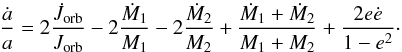 (1)For conservative mass transfer within circular orbits (e = 0), it is assumed that mass and orbital angular momentum are conserved, i.e. Ṁ2 = −Ṁ1, and
  (e.g. Paczyński 1971). Here, mass transfer from the more massive primary to the less massive secondary (q = M1/M2> 1) leads to orbital shrinkage (ȧ< 0), while the reverse occurs for q< 1 (see, e.g. Pringle & Wade 1985). However, even if the mass remains in the system, orbital angular momentum may not be conserved (
 ) because of the exchange of angular momentum between the orbit and the stellar spins via tidal torques and mass transfer (Gokhale et al. 2007; Deschamps et al. 2013).
In the 60s, several works from Piotrowski (1964), Kruszewski (1964b) and Hadjidemetriou (1969a,b) evaluated the gravitational force between the material leaving the inner-Lagrangian, ℒ1, point (the matter stream) and each star. As a particle travels, it generates a time-varying torque on the stars, allowing for angular momentum to be exchanged between the transferred material and the orbit. Subsequently, Luk’yanov (2008) demonstrated that orbital angular momentum is conserved only if the stars are point masses, if the gravitational force between the matter stream and the stars is neglected and if the velocity of the ejected (accreted) material is equal in magnitude but in the opposite direction to the orbital velocity of the mass loser (gainer; see Appendix B). In reality, the velocity of the accreted particle is determined by the initial ejection velocity, which in turn depends on the thermal sound speed in the primary’s atmosphere and its rotation rate (Kruszewski 1964a; Flannery 1975).
It is widely assumed that tides enforce the synchronous rotation of the primary with the orbit during RLOF. However, there is observational evidence for super- and sub-synchronously rotating stars in circular binaries (e.g. Habets & Zwaan 1989; Andersen et al. 1990; Meibom et al. 2006; Yakut et al. 2007). Furthermore, Pratt & Strittmatter (1976) and Savonije (1978) argued that if the ejected material removes angular momentum faster than tides can act to synchronize the rotation, the primary star will rotate sub-synchronously and its Roche lobe radius will be affected (e.g. Limber 1963; Sepinsky et al. 2007a).
A sub-synchronously rotating primary may cause the ejected material to be accreted back onto the primary (henceforth termed “self-accretion”), which causes the orbit to shrink even when q< 1 (Sepinsky et al. 2010). Super-synchronous rotation, on the other hand, may have the opposite effect (Kruszewski 1964b; Piotrowski 1964, 1967).
In this investigation, we apply the scheme of Hadjidemetriou (1969a,b), who derived the equations of motion of a binary system using the theory of osculating orbital elements. His scheme accounts for the transfer of linear momentum between the stars, and perturbations to the orbit due to the gravitational attraction between the stars and the mass transfer stream. Using our binary stellar evolution code BINSTAR, we calculate the resulting evolution of Algol binaries for a range of initial periods and masses. Currently, we assume that none of the exchanged mass leaves the system. Torques applied onto each star by tides and mass transfer are also included.
The paper is organized as follows. In Sect. 2 we introduce the formalism of Hadjidemetriou (1969a,b). Our results are presented in Sect. 3, and discussed in Sect. 4. We summarise and conclude our investigations in Sect. 5.
2. Computational method
BINSTAR is an extension of the single-star evolution code STAREVOL. Details on the stellar input physics can be found in Siess (2010), and references therein, while the binary input physics is described in Siess et al. (2013) and Deschamps et al. (2013). In this section we present our new implementation of the osculating scheme.
2.1. Variation of the orbital parameters
Consider a binary system with an eccentricity e. The stars orbit about their common centre of mass  (see Fig. 1) with an orbital angular speed, ω, and orbital period Porb.
Material is ejected from the primary star at a rate Ṁ1 with a velocity V1 relative to the primary’s mass centre, given by  (2)where W1 is the absolute velocity of the ejected material, and v1 is the orbital velocity of the primary’s mass centre. Similarly, the velocity of the accreted material V2 with respect to the secondary’s mass centre is
 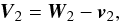 (3)where W2 is the absolute velocity of the accreted material, and v2 is the secondary’s orbital velocity. Ejection occurs from the ℒ1 point, located at a distance rℒ1 from the primary’s centre. The Roche radius Rℒ1 and rℒ1, are calculated as in Davis et al. (2013), using the formalism described by Sepinsky et al. (2007a), that accounts for the donor’s rotation.
The impact site is located at racc with respect to the secondary’s centre of mass. The distance racc is either the secondary’s radius, R2, for direct impact accretion or the accretion disc radius. The latter is estimated from the distance of closest approach of the accretion stream to the secondary, rmin, and is given by  (4)(Lubow & Shu 1975; Ulrich & Burger 1976), where rmin is determined from our ballistic calculations (see Sect. 2.3). The vector racc forms an angle
  (5)with the line joining the two stars, êr (Fig. 1).
 |
Fig. 1 Schematic of a binary system, consisting of a primary star of mass M1, and a secondary of mass M2 orbiting with an angular speed ω, where the centre of mass of the binary system is located at |


In the theory of osculating elements, the rate of change of the semi-major axis, ȧ, and of the eccentricity, ė, can be expressed as (see, e.g. Sterne 1960) ![Mathematical equation: \begin{equation} \dot{a}=\frac{P_{\mathrm{orb}}}{\pi(1-e^{2})^{\frac{1}{2}}}\left[\mathcal{S}e\sin\nu+\mathcal{T}(1+e\cos\nu)\right]\label{eq:adot_osc} \end{equation}](/articles/aa/full_html/2014/10/aa23730-14/aa23730-14-eq48.png) (6)and
(6)and ![Mathematical equation: \begin{equation} \dot{e}=\frac{P_{\mathrm{orb}}(1-e^{2})^{\frac{1}{2}}}{2\pi a}\left\{ \mathcal{S}\sin\nu+\mathcal{T}\left[\frac{2\cos\nu+e(1+\cos^{2}\nu)}{1+e\cos\nu}\right]\right\}, \label{eq:edot_osc} \end{equation}](/articles/aa/full_html/2014/10/aa23730-14/aa23730-14-eq49.png) (7)where
(7)where  and
and  are the perturbing forces per unit mass, acting along êr, and perpendicular to that line (along êt), respectively, and ν is the true anomaly.
To account for the fact that the primary’s sub-synchronous rotation may cause a fraction αself of ejected matter to be self-accreted, we decompose and into two contributions; that resulting from accretion onto the secondary, and that arising from self-accretion. If  and
and  are the mass transfer rates onto the primary and towards the secondary, respectively, then
  (8)The mass accretion rate onto the secondary is
  , where β is the accretion efficiency (β = 1 for conservative mass transfer). The corresponding perturbing forces,
  and
and  , are respectively
 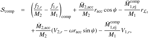 (9)and
 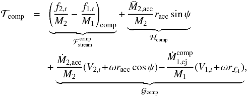 (10)(Hadjidemetriou 1969b; Sepinsky et al. 2007b). The subscripts “r” and “t” refer to the radial and transverse components (i.e. along êr and êt) of the vector quantities, respectively. In Eqs. (9) and (10), terms proportional to fi are the gravitational forces per unit mass acting on the ith star due to the mass transfer stream (see Sect. 2.4), and terms proportional to Ṁi are associated with the change of linear momentum for the ith star, while terms proportional to
  represent the acceleration of the mass centre of the ith star arising from asymmetric mass loss or gain. In Eq. (10),
  ,
,  and ℋcomp correspond respectively to the gravitational force acting on the secondary by the mass transfer stream, the linear momentum transferred to the secondary and the acceleration of its mass centre, all with respect to the primary (see Sect. 3).
The self-accretion rate back onto the primary is  . The associated perturbing forces,
  and
and  , are found by considering the total acceleration experienced by the primary resulting from the ejection and re-capture of material (see Appendix A), giving
 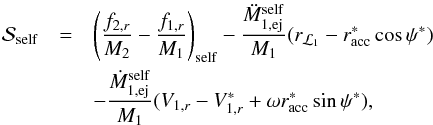 (11)and
 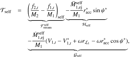 (12)where the asterisks indicate quantities calculated at self-accretion. Here,
  is similar to but now for the self-accreted material, while
  and ℋself correspond respectively to the net momentum transferred to the primary by the ejected and self-accreted material, and the acceleration of its centre of mass. The radius
  is determined from the ballistic calculations, and corresponds to the location of the particle where the Roche potential is equal to the potential at the ℒ1-point. Using Eqs. (9) to (12), the total perturbing forces are
  and
and  .
.
For circular orbits, ȧ is only a function of . For infinitesimal changes of a and e over one orbital period, the term in braces in Eq. (7) averages to zero over one orbit, so ė = 0 (Hadjidemetriou 1969b). Therefore, in the remainder of Sect. 2, we will just describe the quantities pertinent to the calculation of .
The total angular momentum of the binary system, J, is the sum of the spin angular momenta of each star, J1,2, the orbital angular momentum, Jorb, and the angular momentum carried by the mass that is not attached to the stars (i.e. the mass in the wind and in the mass transfer stream), JMT, i.e.  (13)The rate of change of the orbital angular momentum, , is then determined by taking the time derivative of Eq. (13), and solving for , giving
 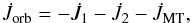 (14)where
 ![Mathematical equation: \begin{eqnarray} \dot{J}_{\mathrm{MT}} & = & \underbrace{-J_{\mathrm{orb}}\left[\frac{\dot{M}_{1,\mathrm{ej}}^{\mathrm{comp}}}{M}\left(\frac{1}{q}-\beta{q}\right)\right]-m a\mathcal{T}}_{\dot{J}_{\mathrm{RLOF}}}\nonumber \\ & & \underbrace{-J_{\mathrm{orb}}\left(\frac{\dot{M}_{1,\mathrm{loss}}}{M}\frac{1}{q}+\frac{\dot{M}_{2,\mathrm{loss}}}{M}q \right)}_{\dot{J}_{\mathrm{lost}}} \label{Jdot_stream} \end{eqnarray}](/articles/aa/full_html/2014/10/aa23730-14/aa23730-14-eq92.png) (15)for circular orbits (see Appendix B). Here, m = M1M2/ (M1 + M2) is the reduced mass, Ṁ1,2,loss< 0 is the systemic mass loss rate from each star (either via winds and/or non-conservative evolution),
(15)for circular orbits (see Appendix B). Here, m = M1M2/ (M1 + M2) is the reduced mass, Ṁ1,2,loss< 0 is the systemic mass loss rate from each star (either via winds and/or non-conservative evolution),  is the torque resulting from the material transferred between the stars, and
  is the torque generated by the material leaving the system (and thus associated with Ṁ1,2,loss). The expression for is identical to that of Bonačić Marinović et al. (2008), which considers that the escaping material carries the specific orbital angular momentum of the star.
For brevity, we term our formalism the osculating scheme. If the stars are point masses, and the gravitational attraction exerted by the accretion stream is neglected, as is usually assumed, then for conservative mass transfer  in Eq. (15) and we recover the classical formulation1.
2.2. Stellar torques
The torques acting on the ith star can be decomposed into the tidal torque  , and the torque arising from mass ejection or accretion,
  , to give
  (16)For stars with radiative envelopes, we apply the prescription for dynamical tides described by Zahn (1989). For convective stars, we use the formalism of Zahn (1977) describing equilibrium tides (see Siess et al. 2013, for further details). For
  we have
  (17)(Piotrowski 1964; Flannery 1975) where Ui,t and Ui,r are the tangential and radial components of the ejection or accretion velocity with respect to a frame of reference co-rotating with the binary, ri is the distance from the ith star’s mass centre to the mass ejection/accretion point (i.e. rℒ1 or racc), φ is the angle between the ejection/accretion point and the line joining the two stars, and Ṁi is the mass loss/accretion rate. From Eq. (17), the torque applied onto the primary because of mass ejection is
  (18)where we have used the fact that φ = 0. The torque arising from self-accretion is
 ![Mathematical equation: \begin{equation} \dot{J}_{\dot{M}_{1}}^{\mathrm{self}}=\dot{M}_{1,\mathrm{acc}}^{\mathrm{self}}\left[\omega (r_{\mathrm{acc}}^{*})^{2}+U^{*}_{1,t}\,r^{*}_{\mathrm{acc}}\cos\phi^{*}-U^{*}_{1,r}\,r^{*}_{\mathrm{acc}}\sin\phi^{*}\right], \label{Jdot_self} \end{equation}](/articles/aa/full_html/2014/10/aa23730-14/aa23730-14-eq110.png) (19)while the torque applied onto the secondary is
(19)while the torque applied onto the secondary is  (20)As shown by Packet (1981), accretion may rapidly spin up the secondary to its critical angular velocity
  . Deschamps et al. (2013) argued that super-critical rotation can be avoided either by the interaction between the secondary and an accretion disc, or magnetic braking (wind braking and disc-locking). For simplicity, we mimic these mechanisms by forcing the secondary’s spin to remain below
  . This translates into an effective torque on the gainer given by
 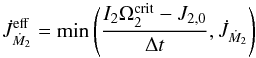 (21)where Δt is the evolutionary time step, which is constrained using the nuclear burning timescales, changes in the stars’ structures, the rates of change of the orbital parameters and the mass transfer rate (see Siess et al. 2013, for further details). Also, I2 is the secondary’s moment of inertia and J2,0 is the secondary’s angular momentum at the previous time step. For simplicity, we assume that each star rotates as a solid body, since the treatment of differential rotation is beyond the scope of this investigation (but see Sect. 4).
2.3. Ejection and accretion velocities
The components of V1 and V2 along êt, i.e. V1,t and V2,t, respectively are given by (Hadjidemetriou 1969b) 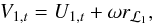 (22)and
 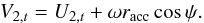 (23)For particles ejected from the ℒ1 point, we set U1,r to the sound speed, cs, at the primary’s photosphere, and U1,t is calculated from
 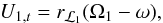 (24)where Ω1 is the spin angular velocity of the primary. We evaluate ψ,U2,r and U2,t by solving the restricted three-body equations of motion (e.g. Hadjidemetriou 1969a; Flannery 1975).
2.4. Perturbing forces from the accretion stream
We discretize the mass transfer stream as a succession of individual particles of mass δmi. The force exerted onto the jth star by the ith particle is 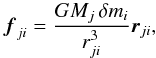 (25)where rji is the distance between the ith particle and star j. In the transverse direction, we have for the primary
 ![Mathematical equation: \begin{equation} r_{1i}=\left\{ [x_{i}-(1-\mu)a]^{2}+y_{i}^{2}\right\} ^{\frac{1}{2}} \end{equation}](/articles/aa/full_html/2014/10/aa23730-14/aa23730-14-eq134.png) (26)and for the secondary
(26)and for the secondary ![Mathematical equation: \begin{equation} r_{2i}=\left[(x_{i}-\mu a)^{2}+y_{i}^{2}\right]^{\frac{1}{2}} \end{equation}](/articles/aa/full_html/2014/10/aa23730-14/aa23730-14-eq135.png) (27)where μ ≡ M1/ (M1 + M2) and (xi,yi) are the coordinates of particle i in the co-rotating frame. Summing Eq. (25) over all stream particles, and taking the difference between the gravitational force (per unit mass) acting on the secondary and on the primary star gives
(27)where μ ≡ M1/ (M1 + M2) and (xi,yi) are the coordinates of particle i in the co-rotating frame. Summing Eq. (25) over all stream particles, and taking the difference between the gravitational force (per unit mass) acting on the secondary and on the primary star gives 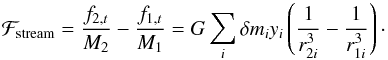 (28)During a time-step δt of the ballistic calculation, the mass contained in the stream that falls towards the secondary is given by
 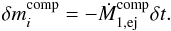 (29)Inserting Eq. (29) into Eq. (28), then in the limit δt → 0, writes as
 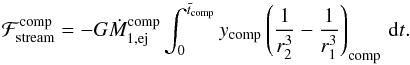 (30)Similarly for the stream falling back onto the primary, we have
 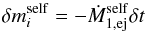 (31)giving
 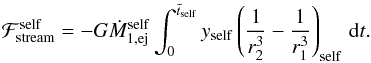 (32)In Eqs. (30) and (32),
  is the particle’s travel time between the ℒ1 point and the point of impact, and r1, r2, and y describe the position of the particle at time t, given by our integration of the ballistic trajectories. The subscripts “comp” and “self” indicate quantities pertaining to material falling onto the secondary and onto the primary, respectively.
2.5. Treatment of the mass transfer stream
The finite width of the matter stream that is ejected from the ℒ1-point is accounted for when calculating the quantities found in Eqs. (10) and (12) as described below. For a primary with an effective temperature Teff,1, mean molecular weight at the photosphere μph,1, the surface area,  , of the stream at the ℒ1 point is
 ![Mathematical equation: \begin{equation} \mathcal{A}=\frac{2\pi\mathcal{R}T_{\mathrm{eff,1}}}{\mu_{\mathrm{ph,1}}}\frac{a^{3}q}{GM_{1}}\left\{g(q)[g(q)-f-qf]\right\}^{-1/2}, \label{Q_area} \end{equation}](/articles/aa/full_html/2014/10/aa23730-14/aa23730-14-eq152.png) (33)(Davis et al. 2013) where ℛ is the ideal gas constant. In Eq. (33),
(33)(Davis et al. 2013) where ℛ is the ideal gas constant. In Eq. (33), ![Mathematical equation: \begin{equation} g(q)=\frac{q}{(r_{\mathcal{L}_{1}}/a)^{3}}+\frac{1}{[1-(r_{\mathcal{L}_{1}}/a)]^{3}}, \label{g_q} \end{equation}](/articles/aa/full_html/2014/10/aa23730-14/aa23730-14-eq154.png) (34)(Kolb & Ritter 1990) and
(34)(Kolb & Ritter 1990) and  (35)corrects for any effects arising from the primary’s rotation.
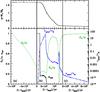 |
Fig. 2 Evolution in time (since the start of mass transfer at tRLOF = 9.62034 × 10⁷ yr) of the primary’s spin angular velocity in units of the orbital velocity, Ω1/ω (dotted green curve, left axis), for the 5 + 3 M⊙ system, initial period Pi = 7 d, using the osculating formalism. Panel a): as the primary evolves off the main sequence up to the onset of mass transfer; panel b): during the self-accretion phase; panel c): during the slow mass transfer phase. Panel b) also shows the fraction of ejected material that falls back onto the primary, αself (solid black curve, left axis), and the ratio of the tidal synchronization timescale to the mass transfer timescale, τsync/τṀ (dashed blue curve, right axis). Note the change in scales along the x-axis in each panel. The top panels indicate the evolution of q = M1/M2, and the open red square indicates where q = 1. |
We then calculate the ballistic trajectory of N particles, which are ejected at evenly spaced intervals, Δℓ, along the width of the ℒ1-point,  . To account for the Gaussian density distribution of the particles at the ℒ1 nozzle (see, e.g. Lubow & Shu 1975; Edwards & Pringle 1987; Raymer 2012) we weight each trajectory using
  (36)where
  is the normalised distance along the finite width of the stream (the ℒ1-point is located at
  ), σ is the standard deviation and η is a normalisation constant set by the requirement that
  . We use σ = 0.4 so that the density at
  and
and  is equal to the donor’s photospheric density, and use N = 128 particles. We checked that increasing N any further or slightly varying σ has negligible impact on the calculations.
Since we are dealing with more than one particle landing on each star, we calculate the average stream properties as follows. Let 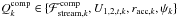 be some quantity related to the kth particle that is ejected from
  , which is subsequently accreted by the companion. Then the mean value of this quantity for a given model is calculated using
  (37)where Ncomp is the number of particles landing on the companion. A similar expression for the particles landing on the donor is used, where we replace “comp” with “self”. Hence, we replace
  , U1,2,t,
  ,
,  and ψ(∗) in Eqs. (10) and (12) with the corresponding mean values, as determined by Eq. (37). Finally, the fraction of particles landing back on the donor star is
  (38)where Nself is the number of particles undergoing self-accretion (N = Nself + Ncomp).
 |
Fig. 3 Left: evolution for the 5 + 3 M⊙ binary system with Pi = 7 d of |


2.6. The binary models
To analyse the impact of this new formalism on the evolution of Algols, we consider two systems. The first configuration is a 5 + 3 M⊙ binary, with an initial period Pi = 7 days, undergoing case B mass transfer (during shell H-burning). Our second system is a 6 + 4 M⊙ binary, Pi = 2.5 days, which commences mass exchange during core H-burning (case A). We assume a solar composition (Z = 0.02), and apply moderate convective core overshooting, with αov = Λ /Hp = 0.2, where Λ is the mixing length and Hp is the pressure scale height. The initial spin periods of each star are set to the initial orbital periods at the start of the simulation (i.e. f = 1 in Eq. (35)) and the orbits are circular.
3. Results
Section 3.1 presents our osculating calculations for the case B system, which are compared to calculations determined from the classical scheme (Sect. 3.1.1), followed by case BB (shell He-burning) mass transfer in Sect. 3.1.2. Calculations for the case A model are given in Sect. 3.2.
3.1. 5 + 3 M⊙, Pi = 7 days
3.1.1. Case B mass transfer
As the primary evolves off the main sequence, its radius and moment of inertia increase on a much shorter timescale (τR = R/Ṙ ≈ 108 yr) than tides can maintain synchronization ( yr) and Ω1 declines (Fig. 2a). Therefore, mass transfer starts while the primary star is rotating significantly sub-synchronously, and this has two important consequences. First, the Roche radius calculated using the Sepinsky et al. (2007a) formalism is 7 per cent larger than the Eggleton (1983) prescription. Consequently, the primary must evolve further along the sub-giant branch before it can start transferring mass. Secondly, at the onset of RLOF, all the material ejected by the primary star is initially self-accreted (αself = 1, panel b, solid black curve). This process induces a positive torque onto the primary (Eq. (19)), increasing Ω1 (dotted green curve) and thus U1,t, causing material to progressively flow onto the companion (αself< 1). In parallel, mass ejected through the ℒ1-point applies a negative torque onto the primary (Eq. (18)). Since, initially, more material is falling onto the primary than onto the companion, the net effect is an acceleration of the primary’s rotation rate, i.e.
  , and a reduction in the amount of self-accreted material. As Ω1 increases,
  drops until eventually the net torque applied onto the primary via the ejection and self-accretion process is zero, i.e.
  . This situation is characterized by a plateau in αself ≈ 0.2. Throughout the self-accretion process, the mass loss timescale τṀ = M1/ | Ṁ1 | <τsync, so tides are unable to enforce synchronous rotation (dashed, blue curve).
For circular orbits, Eq. (6) reduces to  (39)and so the sign of ȧ depends on the signs of and . To understand the evolution of the separation, we show in Fig. 3 the various contributions entering the expression for
  , i.e. the gravitational force applied onto the secondary (primary) by the ejected particle
  , and the linear momentum transferred to the companion (donor),
  , all with respect to the donor. Throughout mass transfer, the terms ℋself and ℋcomp, corresponding to the acceleration of the donor’s or companion’s mass centre, are negligible because
  , and for this reason it is not displayed in Fig. 3. At the start of mass transfer, the contribution to partially comes from (Fig. 3a, left panels, red short-dashed curves), which is negative for two reasons. Firstly, the particles are located at ycomp< 0 and secondly they are typically situated in the vicinity of the secondary i.e. 1 /r2> 1 /r1 (see Eq. (30)).
The term (green, long-dashed curves) is small for q> 1, but increases as q declines. Indeed, as mass transfer proceeds, the primary’s Roche lobe radius and therefore rℒ1 shrink, and so the ℒ1 point moves further away from the companion’s surface. A particle’s travel time thus rises and it can accelerate to a larger impact velocity (V2,t). Even though also depends on V1,t + ωrℒ1, its magnitude is about a factor of 10 smaller than the | V2,t + ωracccosψ | term.
During self-accretion, is dictated by (Fig. 3b). We find that V1,t ≈ − 1 × 107 cm s-1 and  cm s-1, which, for small ψ∗, gives
  (Eq. (12)). Similarly to ,
  because yself< 0 and, owing to the large value of rℒ1 for q> 1, the particle is closer to the secondary than to the primary.
Hence, self-accretion enhances the rate of shrinkage of both the orbital separation (Fig. 3c) and the primary’s Roche radius. This faster contraction of Rℒ1 increases the overfilling factor resulting in a mass transfer rate that is a factor of ~1.6 higher than in the classical scheme. In response to this higher mass loss rate, the primary’s radiative layers further contract and it attains a lower surface luminosity on the Hertzsprung-Russel (HR) diagram compared to the classical calculation (Fig. 4a).
To quantify the impact of self-accretion, we re-ran a simulation by setting  , as indicated by the short-dashed green curve in Fig. 4d. Differences in the mass transfer rate and the evolution along the HR diagram are negligible. However, the post-mass transfer orbital period (about 21 d) is slightly longer than when self-accretion is included (17 d); a relative difference of about 20 per cent.
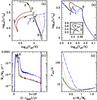 |
Fig. 4 Evolution of the 5 + 3 M⊙ system, Pi = 7 d, calculated using the osculating (solid black curves) and the classical (dotted red curves) prescriptions. The short-dashed green and the long-dashed blue curves also use the osculating scheme, but |
As mass transfer proceeds, τsync decreases as a result of the deepening of the primary’s surface convection zone in response to mass loss (Webbink 1977a). Eventually, τsync<τṀ (Fig. 2b), and tides can re-synchronize the primary. Moreover, as the primary’s mass declines, it exerts a smaller gravitational attraction onto the ejected particle, and evermore material falls onto the secondary star, as indicated by the decrease in αself.
Once q ≲ 1, self-accretion shuts off and soon after (when q ≃ 0.9) becomes positive, allowing the orbit to expand. The rise in is because of the aforementioned growth of the term, resulting from the higher impact velocity (V2,t). Eventually, the primary restores thermal equilibrium, Ṁ1 declines (Fig. 4c) and the evolution enters the slow phase (around q ≈ 0.16), where mass transfer occurs on the nuclear timescale of the hydrogen-burning shell (Paczyński 1971). The calculated mass transfer rates for the classical and osculating models are virtually identical, since the shell-burning properties in both cases are the same2. Also note that throughout the slow phase, τsync ≪ τṀ and so tides can enforce synchronous rotation of the primary (Fig. 2c).
By the end of the simulations, the difference in the periods is significant with 17 days for the osculating scheme compared to 71 days for the classical model. The primary’s radius is correspondingly smaller, since it keeps track of its Roche lobe, which is a function of a. This explains why, for a given luminosity, the osculating model gives a hotter primary than in the classical case (Fig. 4a).
The shorter orbital period predicted by the osculating scheme is caused by the negative contribution. Indeed, neglecting this term gives  , yielding the longest post-mass transfer orbital periods out of all our calculations (Fig. 4d, long-dashed blue curve). In this case, the Roche filling primary has a larger radius and a lower effective temperature, causing a substantial surface convection zone to develop (radial extent of about 60 R⊙). This enhances the mass transfer rate because convective layers expand upon mass loss, causing the star to over-fill its Roche lobe further.
When He ignites in the primary, mass transfer terminates and the final masses are virtually identical between the classical and osculating schemes (M1 ≈ 0.87 M⊙, M2 ≈ 7.3 M⊙).
Both the osculating and classical formalisms predict similar evolutionary tracks of the secondary on the HR diagram (Fig. 4b). Once mass transfer enters the slow phase, the secondary relaxes towards thermal equilibrium, establishing a new effective temperature and luminosity along the main sequence which is appropriate for its new mass.
3.1.2. Case BB mass transfer
Once mass transfer has stopped, the structure of the primary consists of a convective He-burning core of 0.27 M⊙, surrounded by a radiative envelope of ~ 0.60 M⊙. The H-burning shell is located at mass coordinate Mr ≈ 0.73 M⊙, and has a mass of about 0.06 M⊙. When He ignites in the core, the primary contracts within its Roche lobe on a timescale much shorter than τsync leading to super-synchronous rotation (Fig. 5, left panel, solid green curve). The star accelerates up to approximately 3 per cent of the critical velocity when Ω1/ω ≈ 12. These calculations therefore predict the presence of rapidly rotating core-He burning stars in detached binaries. To the best of our knowledge, there are no available observations of such systems in this evolutionary phase.
At about 2.72 × 10⁷ yr since the start of case B mass transfer, the activation of shell-He burning produces a rapid expansion of the primary. As the star fills more of its Roche lobe (R1/Rℒ,1, dashed cyan curve) the tidal forces strengthen and within ~ 1.5 × 10⁶ yr, the primary is re-synchronized. The ensuing case BB (Fig. 5, shaded region) is characterized by a constant mass exchange rate of about 10-7M⊙ yr-1, and an expansion of the orbit because q< 1. Synchronous rotation is maintained during the entire phase of mass transfer, so no self-accretion occurs. In both schemes, mass transfer lasts for about 3 × 10⁵ yr.
Mass transfer ceases as a result of re-ignition of the H-burning shell, which causes the primary’s radius to shrink. At this point, the binary consists of a 0.8 M⊙ CO star, undergoing H-shell burning in the surface layers, and a 7.2 M⊙ main sequence companion. The final orbital periods are approximately 80 days and 19 days for the classical and osculating calculations, respectively.
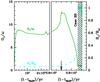 |
Fig. 5 Similar to Fig. 2, but now during core He burning (left panel), and shell He-burning (right panel), the onset of which is indicated by the arrow. The dashed cyan curve shows R1/Rℒ,1 (right axis), and the shaded region marks case BB mass transfer. |
To calculate the subsequent evolution of this system is beyond the scope of the investigation. Nonetheless, we can infer its fate based on the binary parameters. Eventually, the secondary star will evolve off the main sequence, fill its own Roche lobe and transfer mass back to the CO primary star. For the osculating scheme, we estimate that the secondary will fill its Roche lobe with a radius of about 34 R⊙ as it is crossing the sub-giant branch, and for the classical scheme, when the star approaches the base of the giant branch with a radius of ~ 60 R⊙. Because of the high mass ratio M2/M1 ≈ 8, which lies well above the critical value of between 1.2 and 1.3 for dynamically unstable mass transfer (Webbink 2008), we therefore expect this system to enter common envelope evolution.
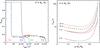 |
Fig. 6 a) Evolution of αself as a function of time, tself, since the start of self-accretion for a 5 + 3 M⊙ system, with an initial orbital period, Pi of 3 d (dotted red curve), 7 d (solid black), 10 d (green short dashed) and 13 d (blue long-dashed). b) Evolution of the orbital period, Porb, as a function of q = M1/M2, for different initial orbital periods: 3 d (dot-dashed); 7 d (solid); 10 d (short-dashed) and 13 d (dotted). Black curves refer to classical calculations, and the red lines to the osculating scheme. |
3.1.3. Effect of changing the initial orbital period
Figure 6a shows that αself levels off to between 0.15 and 0.2 for the considered values of Pi. In addition, the duration of the self-accretion phase progressively decreases, from 5.2 × 10⁴ to 2.6 × 10⁴ yr when the initial period, Pi, rises from 7 to 13 d. By increasing Pi, the primary evolves further along the sub-giant branch before mass transfer starts, and can develop a deeper convection zone. When RLOF occurs, tides are more efficient at re-synchronizing the primary, and self-accretion is stopped earlier.
For Pi between 7 and 13 days, αself ≈ 1 at the start of mass transfer. By contrast, for Pi = 3 d, αself rises from zero to a constant value of approximately 0.2. In this case, the primary is still very close to its main sequence location in the HR diagram, and it is initially not rotating sufficiently slowly to trigger self-accretion. Only once enough angular momentum has been removed from the primary does self-accretion occur.
The final primary masses are between 0.85 and 0.88 M⊙ and the secondary masses between 7.15 and 7.12 M⊙, irrespective of whether the classical or the osculating scheme is used. However, the osculating scheme systematically yields shorter post-mass transfer orbital periods, by a factor of about 4 (Fig. 6b), and for the model with Pi = 3 d, it gives rise to a contact system, in contrast to the classical scheme.
3.2. 6 + 4 M⊙, Pi = 2.5 d
Since the initial period is shorter for this model, tides are able to establish synchronous rotation by the time the primary fills its Roche lobe (Fig. 7a). Therefore, all ejected mass is initially accreted onto the companion (αself = 0) and only once mass ejection has removed a sufficient amount of angular momentum from the primary does self-accretion occur, with αself ≈ 0.15.
As we remarked, self-accretion enhances the orbital contraction because of the negative contribution from (right panel, Fig. 3b). In contrast to the case B model, this process continues after the mass ratio has reversed and only ceases when q ≈ 0.6. The reason for this difference stems from the time delay associated with the appearance of a surface convection zone, which reinforces the tidal interaction and accelerates the primary’s rotation velocity back to synchronous rotation. This persisting self-accretion episode maintains for a longer period of time and the orbit contracts until q ≈ 0.8 (Fig. 3c). Also note that  when q< 1 because the ejected material is typically located in the vicinity of the primary (1 /r1> 1 /r2 in Eq. (32)), owing to the close proximity of the ℒ1-point to the primary. The positive value for , on the other hand, is because the primary’s sub-synchronous rotation deflects the particles such that they have ycomp> 0.
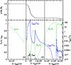 |
Fig. 7 Similar to Fig. 2, but now for the 6 + 4 M⊙ system, Pi = 2.5 days. Here, tRLOF = 6.12305 × 10⁷ yr. |
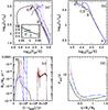 |
Fig. 8 Similar to Fig. 4 but for the 6 + 4 M⊙, Pi = 2.5 d system. A: start of case A mass transfer; B: q = 1; C: end of core H-burning; D: start of shell H-burning; E: end of case A mass transfer (H-shell burning ceases). |
At t ≈ tRLOF + 1 × 10⁶ yr (q ≈ 0.3), the convection zone recedes and τsync rises again (Fig. 7b). Subsequent mass ejection brings the primary back into sub-synchronous rotation, triggering a second self-accretion episode, with about 10 per cent of the ejected material falling back onto the star. This second self-accretion event is absent in the case B model because of the higher sound speed (U1,r) for the primary. The impact of this second occurrence on the orbital evolution, however, is negligible. This is because and  are respectively a factor of about 10 and 6 smaller than the values for the first self-accretion episode. Neglecting (short-dashed green curve, Fig. 8d) shows that the relative difference between the post-mass transfer orbital periods with and without self-accretion is about 15 per cent.
As the mass transfer rate decelerates, τsync/τṀ correspondingly declines, Ω1 increases back towards synchronous rotation and self-accretion shuts off. Eventually, hydrogen is exhausted in the core, the primary shrinks within its Roche lobe, and mass transfer is terminated (giving rise to the hook feature around log 10(L/L⊙) ≃ 2.5 in Fig. 8a). Mass exchange resumes once the primary re-expands because of H-shell ignition. Since now τsync/τṀ ≪ 1, synchronous rotation is maintained throughout the subsequent mass transfer episode which starts at t = tRLOF + 5 × 10⁶ yr (Fig. 7c).
Upon He-core ignition, the final mass of the osculating primary is marginally less massive (≈ 0.9 M⊙) than in the classical models (1.0 M⊙), the total system mass being held constant. As with the case B model, however, the osculating scheme gives a final orbital period which is a factor of 5.5 smaller (≈6 d) than the classical scheme (≈33 d, Fig. 8d).
As for the case B model, is responsible for the shorter post-mass transfer orbital period. The long-dashed blue curve in Fig. 8 presents the evolution if the ℱstream terms are neglected. When q> 1, the orbital separation slightly increases (Fig. 8d) because of the dominant, positive contribution from the ωracccosψ term in Eq. (10). The expansion of the orbit reduces the amount that the primary star over-fills its Roche lobe, giving a correspondingly smaller mass loss rate peaking at about 2 × 10⁻⁷M⊙ yr-1 (Fig. 8c). For a given t − tRLOF, the primary is therefore more massive than found by the other models, and its core-hydrogen burning timescale is, in turn, shorter. By consequence, both shell-hydrogen burning and core-helium burning commence sooner in the binary’s evolution and so the duration of mass transfer is shorter.
Eventually, the secondary will fill its Roche lobe as it evolves off the main sequence, before He-core burning has ceased in the primary. This second mass transfer episode starts when the secondary’s radius is 17 R⊙ for the osculating scheme and 53 R⊙ for the classical model. As for the case B system, we expect common envelope evolution to follow because of the extreme mass ratio.
4. Discussion
4.1. Consequences of the osculating scheme on the orbital evolution
Our simulations show that the osculating scheme yields a significantly shorter post-mass transfer orbital period than the classical formalism. Alternatively expressed, to obtain an Algol with a given orbital period, the osculating prescription requires a longer initial period. Consequently, the progenitor primary may fill its Roche lobe once it has already developed a deep surface convection zone near the base of the giant branch. Tout & Eggleton (1988a) suggested this was the case for a number of observed Algols, for example TW Dra and AR Mon. Mass transfer would therefore proceed on the dynamical – rather than the thermal – timescale, possibly causing common envelope evolution. They proposed, however, that such a fate can be avoided if the primary loses sufficient mass via an enhanced stellar wind (companion-reinforced attrition process; Tout & Eggleton 1988b) to reduce the mass ratio close to unity, before RLOF starts.
We currently consider conservative evolution, which may be a reasonable assumption during the slow mass transfer phase. van Rensbergen et al. (2008) suggested that non-conservative mass transfer in Algols is triggered by a hotspot located at the secondary’s surface, or at the edge of an accretion disc. They further found that this mechanism typically operates during the rapid mass transfer phase, and becomes quiescent within the slow regime. Other suggested mechanisms – albeit poorly studied – include mass escaping through the outer Lagrangian ℒ3 point (Sytov et al. 2007) or by bipolar jets (Ak et al. 2007). The removal of orbital angular momentum via systemic mass losses was also invoked by De Greve et al. (1985) and De Greve & Linnell (1994) to explain the observed orbital periods of TV Cas, β Lyrae and SV Cen. For TV Cas, for example, the authors estimated that 80 per cent of the transferred mass is ejected from the system, removing about 40 per cent of the progenitor’s orbital angular momentum. However, given the effect of ℱstream on the orbital evolution, we argue that a fraction of the estimated orbital angular momentum loss can be attributed to the gravitational interaction between the stars and the mass transfer stream. Therefore, the amount of orbital angular momentum carried by the expelled mass may be lower than quoted by De Greve et al. (1985). We will consider the impact of non-conservative evolution in a future investigation.
Our simulations indicate that, contrarily to what is usually assumed, the primary does not always rotate synchronously throughout mass exchange. As shown in Figs. 2 and 7, the primary is rotating significantly sub-synchronously during the rapid phase. Only once the mass transfer rate decelerates and convection develops in the surface layers, are tides effective enough to re-synchronize the primary.
Unfortunately, published spin rates of the primary during the rapid phase are, to the best of our knowledge, not available, but this is likely a result of the short duration of this phase (between about 105 to 106 years in our models). Existing studies of rapid mass transfer systems, such as UX Mon (Sudar et al. 2011), assume that the primary is synchronous, based upon the expectations that tides are always efficient enough to maintain synchronism, although this has never been proven observationally. On the other hand, evidence for synchronous primaries where the mass ratio has reversed are relatively abundant, such as the eclipsing δ Scuti star KIC 10661783 (Lehmann et al. 2013), TX Uma (Glazunova et al. 2011), KZ Pav (Sürgit et al. 2010) and RX Cas (Andersen et al. 1989).
4.2. Contact evolution
The enhanced orbital contraction that self-accretion generates, combined with expanding radiative secondaries in response to mass accretion (e.g. Neo et al. 1977), could lead to more contact systems. The situation may be particularly severe for case A systems when self-accretion operates even after the mass ratio has reversed. Indeed, even though the classical scheme predicts orbital expansion when q< 1, self-accretion still causes the orbit to contract down to q ≃ 0.8 in our case A simulation. However, contact may be avoided if, for a given initial period, the mass ratio is initially close to unity. In this configuration, the mass ratio is reversed sooner, limiting the orbital shrinkage.
The spin-up of the secondary, as it accretes angular momentum from the transferred material (Packet 1981), may also lead to a contact binary. Sepinsky et al. (2007a) demonstrated that the Roche lobe radius of a super-synchronously rotating star will be smaller than the value determined using the standard Eggleton (1983) formula. So, if we also consider the impact of the secondary’s rotation on its Roche radius (as should be done), we indeed find that all our models enter a contact configuration during the rapid phase. However, magnetic braking may prevent significant spin-up of the secondary (Dervişoǧlu et al. 2010; Deschamps et al. 2013) although, in light of the expanding radiative secondary, these mechanisms may only delay the onset of contact.
Contact evolution requires detailed modelling of energy transport between the stars within their common envelope (e.g. Webbink 1977b; Stȩpień 2009), which is beyond the scope of the present paper. Nonetheless, observations of the contact systems with early spectral-type stars, such as LY Aur (Zhao et al. 2014), V382 Cyg and TU Mus (Qian et al. 2007) indicate that their evolution is similar to that of a semi-detached Algol, but much shorter-lived. The authors suggest that the contact configuration was most likely triggered during a rapid case A mass transfer phase, and that the observed period increase is caused by mass transfer from the less massive to the more massive star. They also expect that the increasing orbital separation will break the contact configuration, giving a semi-detached Algol, suggesting that not all contact systems necessarily merge.
Further complications arise from the fact that the rotation rate of each star is different. The concept of the Roche model, which assumes that both stars rotate synchronously with the orbit, is therefore incorrect. As outlined by Vanbeveren (1977), asynchronous rotation of both components gives Roche lobes that do not necessarily coincide at a common inner-Lagrangian point. This situation may greatly complicate the mass flow structure between the stars, possibly leading to non-conservative evolution. We appeal to smooth particle hydrodynamical (SPH) simulations to investigate this in further detail.
4.3. Physical considerations
4.3.1. Stellar rotation
By adopting the solid-body approximation, we assume that torques will spin up or spin down each star as a whole. However, it is more likely that only the outer-most layers will be affected, thereby triggering differential rotation. Subsequently, angular momentum is re-distributed within the stellar interior via meridional circulation and shear instabilities (see Maeder 2009, for a review).
Song et al. (2013) studied the affect of angular momentum transport within a differentially rotating 15 M⊙ primary, with a 10 M⊙ companion as the primary evolved from the ZAMS until the onset of RLOF. They found that meridional circulation always counteracts the impact of tides; spinning up the surface layers when tides spin them down and vice versa, increasing the time for the star to rotate synchronously with the orbit. Consequently, some of their models commence RLOF before the primary is synchronised. In addition, differential rotation significantly enhances nitrogen abundances at the stellar surface.
We can speculate that significant differential rotation will occur while our donors become sub-synchronous, with meridional circulation initially opposing the spin-down triggered by rapid mass loss, and then the subsequent tidal forces which act to re-synchronise the donor. In turn, this may affect both the duration of the self-accretion phase and the value of αself.
4.3.2. Tides
Tassoul (1987, 1988) proposed an alternative theory that invokes large-scale hydrodynamical flows as a means to dissipate kinetic energy, which are more efficient than the dynamical tide model described by Zahn (1977). Indeed, the synchronization and circularisation timescales between the two approaches vary by up to three orders of magnitude (Khaliullin & Khaliullina 2010).
We can speculate on the impact of Tassoul’s formalism on our calculations as follows. If τsync is 1000 times shorter, then for our case B system τsync<τR, i.e. tides keep the donor in synchronous rotation by the time RLOF starts. Additionally, for both the case A and case B models, an inspection of Figs. 2 and 7 shows that we would have τsync<τṀ. Hence, even during the fast phase, mass loss would not be sufficiently rapid to spin down the donor star to sub-synchronous rates and, in turn, self-accretion would not be triggered. In this case, the orbital evolution will correspond to the short-dashed green curves given in Figs. 4 and 8, where we neglected the term. Therefore, using Tassoul’s formalism will not significantly affect our results, namely that our osculating scheme still yields much shorter orbital periods.
However, the hydrodynamical model has since been criticised on theoretical grounds by Rieutord (1992) and Rieutord & Zahn (1997; but see Tassoul & Tassoul 1997, for a counter-argument), while observations attempting to constrain the mechanism underpinning tidal interactions are inconclusive. On the one hand, Claret et al. (1995) and Claret & Cunha (1997) found that both the Zahn and Tassoul formalisms can adequately account for the observed eccentricities and rotational velocities of early-type eclipsing binaries. On the other hand, using an updated sample of such binaries, Khaliullin & Khaliullina (2007, 2010) found that Tassoul’s theory is in contradiction with observations, which are better reproduced by Zahn’s formalism. However, Meibom & Mathieu (2005) derived, for stellar populations with a range of ages, the tidal circularization period (i.e. the orbital period at which the binary orbit circularises at the age of the population). Their results indicated that, at a given age, the observed circularisation period is larger than the predicted value from the dynamical tide model, suggesting that it is too inefficient. Clearly, more observational and theoretical work is required in this area.
4.3.3. Self-accretion
The phenomenon of self-accretion has also been found in the studies of Kruszewski (1964a) and Sepinsky et al. (2010), who use the same ballistic approach, which assumes that no collisions between particles occur. Clearly, this is not realistic, as there are indeed multiple collisions along the trajectory.
Nonetheless, our results are in qualitative agreement with the SPH calculations of Belvedere et al. (1993), who find that below some critical rotational velocity, the entire stream is deflected towards the primary. For larger spin rates, material falls onto both components. However, their study focused on the impact of asynchronous rotation on disc formation around the secondary, and they did not quantify self-accretion. We hope our work will motivate future SPH studies in this area.
5. Summary and conclusions
We use our stellar binary evolution code BINSTAR to calculate the evolution of Algol systems using the theory of osculating orbital elements. By calculating the ballistic trajectories of ejected particles from the mass losing star (the donor), we determine the change of linear momentum of each star, and the gravitational perturbation applied to the stars by the mass transfer stream. As a consequence of the latter, the osculating formalism predicts signicantly shorter post-mass transfer orbital periods, typically by a factor of 4, than the widely applied classical scheme.
Also contrary to widely held belief, the donor star does not remain in synchronous rotation with the orbital motion throughout mass exchange. The initially rapid mass ejection spins down the donor on a shorter timescale than the tidal synchronization timescale, enforcing sub-synchronous rotation and causing about 15 to 20 per cent of the ejected material to fall back onto the donor during these episodes of self-accretion. Self-accretion, combined with the sink of orbital angular momentum that mass transfer provides, may lead to the formation of more contact binary systems.
While we have mainly focused on conservative Algol evolution, the osculating prescription clearly applies to all varieties of interacting binaries. In the future, we will apply our osculating formalism to investigate the evolution of eccentric systems.
Online material
Appendix A: The perturbing forces  and
and 
Consider a primary star of mass M1. At time t = t0, it has an orbital velocity v1 = v0, and an orbital angular velocity ω. At a later time t = t′, a particle is ejected from the primary at the inner-Lagrangian point, located at a distance rℒ1 from the primary’s mass centre (see Fig. A.1), and so the primary’s mass becomes  , where
  . The particle’s absolute velocity is
  . As a result, the centre of mass is shifted by
 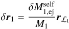 (A.1)with respect to its unperturbed location, and its new orbital velocity is
  . During a time interval δt, the change in the primary’s orbital velocity is (see Hadjidemetriou 1969b; Sepinsky et al. 2007b, for further details)
  (A.2)where Q1 is the primary’s momentum, primed quantities indicate values at time t′, and Vej = Wej − v1 is the relative velocity of the ejected material with respect to the primary’s mass centre.
At self-accretion, the primary accretes the particle of mass  . Just before self-accretion occurs at time t = t′′, the momentum of the primary and ejected particle,
  , is
, is  (A.3)where Wacc is the absolute velocity of the self-accreted particle. The orbital velocity,
  , is the sum of the non-perturbed orbital velocity at time t′′,
  , and the perturbation to the velocity because of the original ejection episode, so
 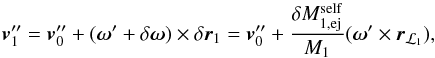 (A.4)
(A.4)
 |
Fig. A.1 Illustration of the self-accretion process. At time t = t0, the donor star moves along its orbital path (solid black curve), with an orbital velocity v0 (cyan arrow). At t′, a particle of mass |

where we have used Eq. (A.1) and ignored terms larger than first-order. Inserting Eq. (A.4) into Eq. (A.3) gives  (A.5)The particle is self-accreted at time t′′′, at a location
  with respect to the primary’s mass centre. This shifts the mass centre by an amount
  (A.6)and the primary’s momentum is now
  (A.7)The new orbital velocity,
  , is the sum of the unperturbed orbital velocity,
  , and the perturbations to the velocity arising from the ejection and self-accretion processes, i.e.
 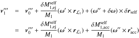 (A.8)where we have used Eq. (A.6), and once again ignored terms higher than first-order. Inserting Eq. (A.8) into Eq. (A.7) yields
  (A.9)Taking the difference between Eqs. (A.9) and (A.5), dividing the result by δt and using the fact that
  yields
 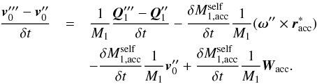 (A.10)Following Sepinsky et al. (2007b), the absolute acceleration of the primary’s mass centre is the sum of Eq. (A.10), the relative acceleration of the primary’s mass centre,
  , and the Coriolis acceleration,
  to give
 ![Mathematical equation: \appendix \setcounter{section}{1} \begin{eqnarray} \frac{\vec{v}_{1}^{\prime\prime\prime}-\vec{v}_{1}^{\prime\prime}}{\delta t}& = & \frac{1}{M_{1}}\frac{\vec{Q}_{1}^{\prime\prime\prime}-\vec{Q}_{1}^{\prime\prime}}{\delta t}+\frac{\delta M_{1,\mathrm{acc}}^{\mathrm{self}}}{\delta t}\frac{1}{M_{1}}[(\vec{\omega}^{\prime\prime}\times \vec{r}_{\mathrm{acc}}^{*})+\vec{V}_{\mathrm{acc}}]\nonumber \\ & & +\frac{1}{M_{1}}\frac{\delta M_{1,\mathrm{acc}}^{\mathrm{self}}}{(\delta t)^{2}}, \label{dV_self} \end{eqnarray}](/articles/aa/full_html/2014/10/aa23730-14/aa23730-14-eq332.png) (A.11)where
(A.11)where  is the relative velocity of the self-accreted particle with respect to the primary’s mass centre.
Summing Eqs. (A.11) and (A.2) gives the acceleration of the primary’s mass centre from both the ejection and self-accretion process. In the limit δt → 0, and remembering that  , then the acceleration of the primary’s mass centre is
 ![Mathematical equation: \appendix \setcounter{section}{1} \begin{eqnarray} \frac{\mathrm{d}^{2}\vec{R}_{1}}{\mathrm{d}t^{2}}& = &\frac{\vec{F}_{1}}{M_{1}}+\frac{\dot{M}_{1,\mathrm{ej}}^{\mathrm{self}}}{M_{1}}\left[(\vec{V}_{\mathrm{ej}}-\vec{V}_{\mathrm{acc}})+(\vec{\omega}^{\prime}\times \vec{r}_{\mathcal{L}_{1}}-\vec{\omega}^{\prime\prime}\times \vec{r}_{\mathrm{acc}}^{*})\right]\nonumber \\ & & +\frac{\ddot{M}_{1,\mathrm{ej}}^{\mathrm{self}}}{M_{1}}(\vec{r}_{\mathcal{L}_{1}}-\vec{r}_{\mathrm{acc}}^{*}), \label{dR1_dt} \end{eqnarray}](/articles/aa/full_html/2014/10/aa23730-14/aa23730-14-eq335.png) (A.12)where R1 is the position vector of the primary with respect to an inertial reference frame, and F1 is the sum of all external forces acting on the primary, which writes as
(A.12)where R1 is the position vector of the primary with respect to an inertial reference frame, and F1 is the sum of all external forces acting on the primary, which writes as  (A.13)where r = R2 − R1, R2 is the position vector of the secondary, and f1 is the force acting on the primary via the matter stream. Since the secondary is not accreting, its equation of motion is
 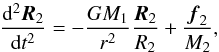 (A.14)where f2 is the force acting on the secondary by the accretion stream. Subtracting Eq. (A.12) from Eq. (A.14) gives the equation of motion of the secondary with respect to the primary, which is
 ![Mathematical equation: \appendix \setcounter{section}{1} \begin{eqnarray} \frac{\mathrm{d}^{2}\vec{r}}{\mathrm{d}t^{2}} & = & -\frac{G(M_1+M_{2})}{r^{3}}\vec{r}+\frac{\vec{f}_{2}}{M_{2}}-\frac{\vec{f}_{1}}{M_{1}}-\frac{\dot{M}_{1,\mathrm{ej}}^{\mathrm{self}}}{M_{1}}\Big[(\vec{V}_{\mathrm{ej}}-\vec{V}_{\mathrm{acc}}) \nonumber \\ & & +\left(\vec{\omega}^{\prime}\times \vec{r}_{\mathcal{L}_{1}}-\vec{\omega}^{\prime\prime}\times \vec{r}_{\mathrm{acc}}^{*}\right)\Big]-\frac{\ddot{M}_{1,\mathrm{ej}}^{\mathrm{self}}}{M_{1}}(\vec{r}_{\mathcal{L}_{1}}-\vec{r}_{\mathrm{acc}}^{*}), \label{dr2_dt2} \end{eqnarray}](/articles/aa/full_html/2014/10/aa23730-14/aa23730-14-eq344.png) (A.15)which takes the form
(A.15)which takes the form 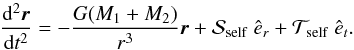 (A.16)Here, êr is a unit vector pointing along r, and êt is a unit vector perpendicular to êr in the direction of the orbital motion. Taking the dot product of Eq. (A.16) with êr and êt respectively, yields
 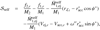 (A.17)and
 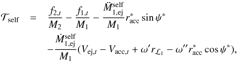 (A.18)which are the same as Eqs. (11) and (12), noting that ω′ = ω′′ = ω for circular orbits. The quantity ψ∗ is the angle between êr and the impact site, and the subscripts “r” and “t” indicate components along êr and êt respectively.
Appendix B: Torque arising from mass transfer, 
Consider a primary star of mass M1, and a secondary of mass M2, separated by a distance r. They respectively orbit the common centre of mass with an orbital velocity v1 and v2. The velocity of the secondary with respect to the primary is v = v2 − v1, and the orbital angular momentum is given by ![Mathematical equation: \appendix \setcounter{section}{2} \begin{equation} J_{\mathrm{orb}}=m\left[GMa\left(1-e^{2}\right)\right]^{1/2}=mrv_{t}, \label{J_orb} \end{equation}](/articles/aa/full_html/2014/10/aa23730-14/aa23730-14-eq352.png) (B.1)where e is the eccentricity, m = M1M2/M is the reduced mass, M = M1 + M2, and vt is the orbital velocity along êt, given by
(B.1)where e is the eccentricity, m = M1M2/M is the reduced mass, M = M1 + M2, and vt is the orbital velocity along êt, given by ![Mathematical equation: \appendix \setcounter{section}{2} \begin{equation} v_{t}=\left[\frac{GM}{a(1-e^{2})}\right]^{1/2}(1+e\cos\nu) \label{vt} \end{equation}](/articles/aa/full_html/2014/10/aa23730-14/aa23730-14-eq356.png) (B.2)and ν is the true anomaly. Taking the time derivative of the last equality in Eq. (B.1) and noting that ṙ = 0 for an osculating orbit (see, e.g. Bonačić Marinović et al. 2008), yields
(B.2)and ν is the true anomaly. Taking the time derivative of the last equality in Eq. (B.1) and noting that ṙ = 0 for an osculating orbit (see, e.g. Bonačić Marinović et al. 2008), yields 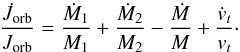 (B.3)Similarly to Eq. (A.16), the equation of motion of a binary acted on by perturbing forces and reads
 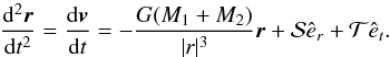 (B.4)Taking the dot product of Eq. (B.4) with êt gives
  (B.5)Inserting Eqs. (B.5) and (B.2) into Eq. (B.3), and using the first equality in Eq. (B.1), gives the torque applied onto the orbit from mass transfer,
 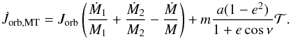 (B.6)The net change of the primary’s mass is the sum of mass transferred to the companion via RLOF,
  , and mass ejected by the wind, Ṁ1,loss< 0, i.e.
 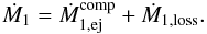 (B.7)Similarly, for the secondary
 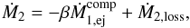 (B.8)where the first term on the right hand side gives the accretion rate and Ṁ2,loss includes the mass ejected from the system during non-conservative mass transfer. Substituting Eqs. (B.7) and (B.8) into Eq. (B.6) gives
 ![Mathematical equation: \appendix \setcounter{section}{2} \begin{eqnarray} \dot{J}_{\mathrm{orb,MT}} & = & \underbrace{J_{\mathrm{orb}}\left[\frac{\dot{M}_{1,\mathrm{ej}}^{\mathrm{comp}}}{M}\left(\frac{1}{q}-\beta{q}\right)\right]+m \frac{a(1-e^{2})}{1+e\cos\nu}\mathcal{T}}_{\dot{J}_{\mathrm{orb,RLOF}}}\nonumber \\ & & +\underbrace{J_{\mathrm{orb}}\left(\frac{\dot{M}_{1,\mathrm{loss}}}{M}\frac{1}{q}+\frac{\dot{M}_{2,\mathrm{loss}}}{M}q\right)}_{\dot{J}_{\mathrm{orb,lost}}} \label{J_orb_3} \end{eqnarray}](/articles/aa/full_html/2014/10/aa23730-14/aa23730-14-eq367.png) (B.9)where q = M1/M2,
(B.9)where q = M1/M2,  is the torque acting on the orbit as a consequence of RLOF, while
  is the torque applied by the material leaving the system. The corresponding torque applied onto the transferred mass is just
 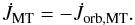 (B.10)Using Eqs. (B.9) and (B.10) with e = 0 gives Eq. (15).
Next, we demonstrate the consistency of Eq. (B.9) by showing that in the classical formalism for conservative mass transfer  . If all material is transferred to the secondary (αself = 0, β = 1), if the stars are treated as point masses (rℒ1 = 0, racc = 0), and if we neglect the gravitational attraction by the accretion stream (f1 = 0, f2 = 0), Eq. (10) reduces to
 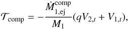 (B.11)where
  for conservative mass transfer. Sepinsky et al. (2007b) and Luk’yanov (2008) demonstrated that, if the
orbital angular momentum is conserved, in a circular orbit V1,t and V2,t are related by 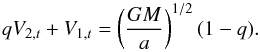 (B.12)Substituting Eq. (B.12) into Eq. (B.11), and that result into Eq. (B.6) gives for a circular orbit
 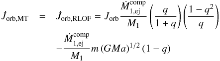 (B.13)where we have used M1/M = q/ (1 + q). Using Eq. (B.1), Eq. (B.13) reduces to zero, as required.
The spike just before mass transfer terminates is due to the ignition of core Helium burning.
Acknowledgments
P.J.D. acknowledges financial support from the FNRS Research Fellowship – Chargé de Recherche. L.S. is a FNRS Research Associate. We thank the anonymous referee whose constructive comments helped to improve the quality of the manuscript.
References
- Ak, H., Chadima, P., Harmanec, P., et al. 2007, A&A, 463, 233 [NASA ADS] [CrossRef] [EDP Sciences] [Google Scholar]
- Andersen, J., Pavlovski, K., & Piirola, V. 1989, A&A, 215, 272 [NASA ADS] [Google Scholar]
- Andersen, J., Nordstrom, B., & Clausen, J. V. 1990, A&A, 228, 365 [NASA ADS] [Google Scholar]
- Belvedere, G., Lanzafame, G., & Molteni, D. 1993, A&A, 280, 525 [NASA ADS] [Google Scholar]
- Bonačić Marinović, A. A., Glebbeek, E., & Pols, O. R. 2008, A&A, 480, 797 [NASA ADS] [CrossRef] [EDP Sciences] [Google Scholar]
- Chen, X., Han, Z., Deca, J., & Podsiadlowski, P. 2013, MNRAS, accepted [arXiv:1306.3281] [Google Scholar]
- Claret, A., & Cunha, N. C. S. 1997, A&A, 318, 187 [NASA ADS] [Google Scholar]
- Claret, A., Gimenez, A., & Cunha, N. C. S. 1995, A&A, 299, 724 [NASA ADS] [Google Scholar]
- Davis, P. J., Siess, L., & Deschamps, R. 2013, A&A, 556, A4 [NASA ADS] [CrossRef] [EDP Sciences] [Google Scholar]
- De Greve, J. P., & Linnell, A. P. 1994, A&A, 291, 786 [NASA ADS] [Google Scholar]
- De Greve, J. P., Packet, W., & de Landtsheer, A. C. 1985, A&A, 142, 367 [NASA ADS] [Google Scholar]
- Dervişoǧlu, A., Tout, C. A., & Ibanoǧlu, C. 2010, MNRAS, 406, 1071 [NASA ADS] [Google Scholar]
- Deschamps, R., Siess, L., Davis, P. J., & Jorissen, A. 2013, A&A, 557, A40 [NASA ADS] [CrossRef] [EDP Sciences] [Google Scholar]
- Edwards, D. A., & Pringle, J. E. 1987, MNRAS, 229, 383 [NASA ADS] [CrossRef] [Google Scholar]
- Eggleton, P. P. 1983, ApJ, 268, 368 [NASA ADS] [CrossRef] [Google Scholar]
- Flannery, B. P. 1975, MNRAS, 170, 325 [NASA ADS] [CrossRef] [Google Scholar]
- Geller, A. M., & Mathieu, R. D. 2011, Nature, 478, 356 [NASA ADS] [CrossRef] [PubMed] [Google Scholar]
- Glazunova, L. V., Mkrtichian, D. E., & Rostopchin, S. I. 2011, MNRAS, 415, 2238 [NASA ADS] [CrossRef] [Google Scholar]
- Gokhale, V., Peng, X. M., & Frank, J. 2007, ApJ, 655, 1010 [NASA ADS] [CrossRef] [Google Scholar]
- Habets, G. M. H. J., & Zwaan, C. 1989, A&A, 211, 56 [NASA ADS] [Google Scholar]
- Hadjidemetriou, J. D. 1969a, Ap&SS, 3, 330 [NASA ADS] [CrossRef] [Google Scholar]
- Hadjidemetriou, J. D. 1969b, Ap&SS, 3, 31 [NASA ADS] [CrossRef] [Google Scholar]
- Han, Z., Podsiadlowski, P., Maxted, P. F. L., Marsh, T. R., & Ivanova, N. 2002, MNRAS, 336, 449 [NASA ADS] [CrossRef] [Google Scholar]
- Hoyle, F., & Fowler, W. A. 1960, ApJ, 132, 565 [NASA ADS] [CrossRef] [EDP Sciences] [Google Scholar]
- Khaliullin, K. F., & Khaliullina, A. I. 2007, MNRAS, 382, 356 [NASA ADS] [CrossRef] [Google Scholar]
- Khaliullin, K. F., & Khaliullina, A. I. 2010, MNRAS, 401, 257 [NASA ADS] [CrossRef] [Google Scholar]
- Kolb, U., & Ritter, H. 1990, A&A, 236, 385 [NASA ADS] [Google Scholar]
- Kruszewski, A. 1964a, Acta Astron., 14, 231 [NASA ADS] [Google Scholar]
- Kruszewski, A. 1964b, Acta Astron., 14, 241 [NASA ADS] [Google Scholar]
- Lehmann, H., Southworth, J., Tkachenko, A., & Pavlovski, K. 2013, A&A, 557, A79 [NASA ADS] [CrossRef] [EDP Sciences] [Google Scholar]
- Leigh, N., Knigge, C., Sills, A., et al. 2013, MNRAS, 428, 897 [NASA ADS] [CrossRef] [Google Scholar]
- Limber, D. N. 1963, ApJ, 138, 1112 [NASA ADS] [CrossRef] [Google Scholar]
- Lubow, S. H., & Shu, F. H. 1975, ApJ, 198, 383 [NASA ADS] [CrossRef] [Google Scholar]
- Luk’yanov, L. G. 2008, Astron. Rep., 52, 680 [NASA ADS] [CrossRef] [Google Scholar]
- Maeder, A. 2009, Physics, Formation and Evolution of Rotating Stars (Berlin, Heidelberg: Springer) [Google Scholar]
- McCrea, W. H. 1964, MNRAS, 128, 147 [NASA ADS] [CrossRef] [Google Scholar]
- Meibom, S., & Mathieu, R. D. 2005, ApJ, 620, 970 [NASA ADS] [CrossRef] [Google Scholar]
- Meibom, S., Mathieu, R. D., & Stassun, K. G. 2006, ApJ, 653, 621 [NASA ADS] [CrossRef] [Google Scholar]
- Mengel, J. G., Norris, J., & Gross, P. G. 1976, ApJ, 204, 488 [NASA ADS] [CrossRef] [Google Scholar]
- Neo, S., Miyaji, S., Nomoto, K., & Sugimoto, D. 1977, PASJ, 29, 249 [NASA ADS] [Google Scholar]
- Packet, W. 1981, A&A, 102, 17 [NASA ADS] [Google Scholar]
- Paczyński, B. 1971, ARA&A, 9, 183 [NASA ADS] [CrossRef] [Google Scholar]
- Paczynski, B. 1976, in Structure and Evolution of Close Binary Systems, eds. P. Eggleton, S. Mitton, & J. Whelan, IAU Symp., 73, 75 [Google Scholar]
- Piotrowski, S. L. 1964, Acta Astron., 14, 251 [NASA ADS] [Google Scholar]
- Piotrowski, S. L. 1967, Sov. Astron., 11, 191 [NASA ADS] [Google Scholar]
- Pratt, J. P., & Strittmatter, P. A. 1976, ApJ, 204, L29 [NASA ADS] [CrossRef] [Google Scholar]
- Pringle, J. E., & Wade, R. A. 1985, Interacting binary stars (Cambridge University Press) [Google Scholar]
- Qian, S.-B., Yuan, J.-Z., Liu, L., et al. 2007, MNRAS, 380, 1599 [NASA ADS] [CrossRef] [Google Scholar]
- Raymer, E. 2012, MNRAS, 427, 1702 [NASA ADS] [CrossRef] [Google Scholar]
- Rieutord, M. 1992, A&A, 259, 581 [Google Scholar]
- Rieutord, M., & Zahn, J.-P. 1997, ApJ, 474, 760 [NASA ADS] [CrossRef] [Google Scholar]
- Savonije, G. J. 1978, A&A, 62, 317 [NASA ADS] [Google Scholar]
- Sepinsky, J. F., Willems, B., & Kalogera, V. 2007a, ApJ, 660, 1624 [NASA ADS] [CrossRef] [Google Scholar]
- Sepinsky, J. F., Willems, B., Kalogera, V., & Rasio, F. A. 2007b, ApJ, 667, 1170 [NASA ADS] [CrossRef] [Google Scholar]
- Sepinsky, J. F., Willems, B., Kalogera, V., & Rasio, F. A. 2010, ApJ, 724, 546 [NASA ADS] [CrossRef] [Google Scholar]
- Siess, L. 2010, A&A, 512, A10 [NASA ADS] [CrossRef] [EDP Sciences] [Google Scholar]
- Siess, L., Izzard, R. G., Davis, P. J., & Deschamps, R. 2013, A&A, 550, A100 [NASA ADS] [CrossRef] [EDP Sciences] [Google Scholar]
- Song, H. F., Maeder, A., Meynet, G., et al. 2013, A&A, 556, A100 [NASA ADS] [CrossRef] [EDP Sciences] [Google Scholar]
- Stȩpień, K. 2009, MNRAS, 397, 857 [NASA ADS] [CrossRef] [Google Scholar]
- Sterne, T. E. 1960, An introduction to celestial mechanics (New York: Interscience Publication) [Google Scholar]
- Sudar, D., Harmanec, P., Lehmann, H., et al. 2011, A&A, 528, A146 [NASA ADS] [CrossRef] [EDP Sciences] [Google Scholar]
- Sürgit, D., Erdem, A., & Budding, E. 2010, MNRAS, 407, 497 [NASA ADS] [CrossRef] [Google Scholar]
- Sytov, A. Y., Kaigorodov, P. V., Bisikalo, D. V., Kuznetsov, O. A., & Boyarchuk, A. A. 2007, Astron. Rep., 51, 836 [Google Scholar]
- Tassoul, J.-L. 1987, ApJ, 322, 856 [NASA ADS] [CrossRef] [Google Scholar]
- Tassoul, J.-L. 1988, ApJ, 324, L71 [NASA ADS] [CrossRef] [Google Scholar]
- Tassoul, M., & Tassoul, J.-L. 1997, ApJ, 481, 363 [NASA ADS] [CrossRef] [Google Scholar]
- Tout, C. A., & Eggleton, P. P. 1988a, ApJ, 334, 357 [NASA ADS] [CrossRef] [Google Scholar]
- Tout, C. A., & Eggleton, P. P. 1988b, MNRAS, 231, 823 [NASA ADS] [CrossRef] [Google Scholar]
- Ulrich, R. K., & Burger, H. L. 1976, ApJ, 206, 509 [NASA ADS] [CrossRef] [Google Scholar]
- van Rensbergen, W., De Greve, J. P., De Loore, C., & Mennekens, N. 2008, A&A, 487, 1129 [NASA ADS] [CrossRef] [EDP Sciences] [Google Scholar]
- Vanbeveren, D. 1977, A&A, 54, 877 [NASA ADS] [Google Scholar]
- Wang, B., & Han, Z. 2012, New A Rev., 56, 122 [Google Scholar]
- Webbink, R. F. 1977a, ApJ, 211, 486 [NASA ADS] [CrossRef] [Google Scholar]
- Webbink, R. F. 1977b, ApJ, 215, 851 [NASA ADS] [CrossRef] [Google Scholar]
- Webbink, R. F. 2008, in Astrophys. Space Sci. Lib. 352, eds. E. F. Milone, D. A. Leahy, & D. W. Hobill, 233 [Google Scholar]
- Yakut, K., Aerts, C., & Morel, T. 2007, A&A, 467, 647 [NASA ADS] [CrossRef] [EDP Sciences] [Google Scholar]
- Zahn, J.-P. 1977, A&A, 57, 383 [NASA ADS] [Google Scholar]
- Zahn, J.-P. 1989, A&A, 220, 112 [NASA ADS] [Google Scholar]
- Zeldovich, Y. B., & Guseynov, O. H. 1966, ApJ, 144, 840 [NASA ADS] [CrossRef] [Google Scholar]
- Zhao, E., Qian, S., Li, L., et al. 2014, New Astron., 26, 112 [NASA ADS] [CrossRef] [Google Scholar]
All Figures
|
Fig. 1 Schematic of a binary system, consisting of a primary star of mass M1, and a secondary of mass M2 orbiting with an angular speed ω, where the centre of mass of the binary system is located at |
| In the text | |
|
Fig. 2 Evolution in time (since the start of mass transfer at tRLOF = 9.62034 × 10⁷ yr) of the primary’s spin angular velocity in units of the orbital velocity, Ω1/ω (dotted green curve, left axis), for the 5 + 3 M⊙ system, initial period Pi = 7 d, using the osculating formalism. Panel a): as the primary evolves off the main sequence up to the onset of mass transfer; panel b): during the self-accretion phase; panel c): during the slow mass transfer phase. Panel b) also shows the fraction of ejected material that falls back onto the primary, αself (solid black curve, left axis), and the ratio of the tidal synchronization timescale to the mass transfer timescale, τsync/τṀ (dashed blue curve, right axis). Note the change in scales along the x-axis in each panel. The top panels indicate the evolution of q = M1/M2, and the open red square indicates where q = 1. |
| In the text | |
|
Fig. 3 Left: evolution for the 5 + 3 M⊙ binary system with Pi = 7 d of |
| In the text | |
|
Fig. 4 Evolution of the 5 + 3 M⊙ system, Pi = 7 d, calculated using the osculating (solid black curves) and the classical (dotted red curves) prescriptions. The short-dashed green and the long-dashed blue curves also use the osculating scheme, but |
| In the text | |
|
Fig. 5 Similar to Fig. 2, but now during core He burning (left panel), and shell He-burning (right panel), the onset of which is indicated by the arrow. The dashed cyan curve shows R1/Rℒ,1 (right axis), and the shaded region marks case BB mass transfer. |
| In the text | |
|
Fig. 6 a) Evolution of αself as a function of time, tself, since the start of self-accretion for a 5 + 3 M⊙ system, with an initial orbital period, Pi of 3 d (dotted red curve), 7 d (solid black), 10 d (green short dashed) and 13 d (blue long-dashed). b) Evolution of the orbital period, Porb, as a function of q = M1/M2, for different initial orbital periods: 3 d (dot-dashed); 7 d (solid); 10 d (short-dashed) and 13 d (dotted). Black curves refer to classical calculations, and the red lines to the osculating scheme. |
| In the text | |
|
Fig. 7 Similar to Fig. 2, but now for the 6 + 4 M⊙ system, Pi = 2.5 days. Here, tRLOF = 6.12305 × 10⁷ yr. |
| In the text | |
|
Fig. 8 Similar to Fig. 4 but for the 6 + 4 M⊙, Pi = 2.5 d system. A: start of case A mass transfer; B: q = 1; C: end of core H-burning; D: start of shell H-burning; E: end of case A mass transfer (H-shell burning ceases). |
| In the text | |
|
Fig. A.1 Illustration of the self-accretion process. At time t = t0, the donor star moves along its orbital path (solid black curve), with an orbital velocity v0 (cyan arrow). At t′, a particle of mass |
| In the text | |
Current usage metrics show cumulative count of Article Views (full-text article views including HTML views, PDF and ePub downloads, according to the available data) and Abstracts Views on Vision4Press platform.
Data correspond to usage on the plateform after 2015. The current usage metrics is available 48-96 hours after online publication and is updated daily on week days.
Initial download of the metrics may take a while.