| Issue |
A&A
Volume 569, September 2014
|
|
|---|---|---|
| Article Number | A1 | |
| Number of page(s) | 18 | |
| Section | Extragalactic astronomy | |
| DOI | https://doi.org/10.1051/0004-6361/201424198 | |
| Published online | 08 September 2014 | |
CALIFA: a diameter-selected sample for an integral field spectroscopy galaxy survey⋆
1
Leibniz-Institut für Astrophysik Potsdam (AIP),
An der Sternwarte 16,
14482
Potsdam,
Germany
e-mail:
This email address is being protected from spambots. You need JavaScript enabled to view it.
2
European Southern Observatory, Karl-Schwarzschild-Str. 2, 85748
Garching b. München,
Germany
3
Instituto de Astrofísica de Andalucía (CSIC),
Glorieta de la Astronomía, s/n,
18008
Granada,
Spain
4
Centro Astronómico Hispano Alemán, Calar Alto, (CSIC-MPG), C/Jesús
Durbán Remón 2-2, 04004
Almería,
Spain
5
Instituto de Astrofísica de Canarias, C/Vía Láctea S/N, 38200
La Laguna, Tenerife,
Spain
6
Dept. Astrofísica, Universidad de La Laguna,
C/ Astrofísico Francisco Sánchez, 38205 La Laguna, Tenerife,
Spain
7
Departamento de Astrofísica y CC. de la Atmósfera, Universidad
Complutense de Madrid, Madrid
28040,
Spain
8
Department of Theoretical Physics and Astrophysics, Faculty of
Science, Masaryk University, Kotlárská 2, 611
37
Brno, Czech
Republic
9
Max-Planck Institute for Astronomy, Königstuhl 17, 69117
Heidelberg,
Germany
10
Instituto de Cosmologia, Relatividade e Astrofísica – ICRA, Centro Brasileiro de
Pesquisas Físicas, Rua Dr. Xavier Sigaud 150, CEP 22290-180, Rio de Janeiro, RJ, Brazil
11
School of Physics and Astronomy, University of St
Andrews, North
Haugh, St Andrews,
KY16 9SS,
UK
12
Zentrum für Astronomie der Universität Heidelberg, Astronomisches Recheninstitut,
Mönchhofstr.
12–14, 69120
Heidelberg,
Germany
13 Instituto de Astronomía, Universidad Nacional Autonóma de
Mexico, A.P. 70-264, 04510, Mexico, D.F.
14
Kapteyn Astronomical Institute, Rijksuniversiteit Groningen, Postbus 800,
9700 AV
Groningen, The
Netherlands
15
INAF – Osservatorio Astrofisico di Arcetri, Largo Enrico Fermi
5, 50125
Firenze,
Italy
16
University of Vienna, Türkenschanzstr. 17, 1180
Vienna,
Austria
17
Institute of Astronomy, School of Physics, University of
Sydney, Sydney
NSW
2006,
Australia
18
Laboratoire d’Astrophysique de Marseille - LAM, Université
d’Aix-Marseille & CNRS, UMR 7326, 38 rue F. Joliot-Curie, 13388
Marseille Cedex 13,
France
19
Departamento de Física, Universidade Federal de Santa
Catarina, PO Box 476,
88040-900
Florianópolis, SC, Brazil
20
Laboratoire GEPI, Observatoire de Paris, CNRS-UMR
8111, Univ. Paris Diderot, 5 place
Jules Janssen, 92195
Meudon,
France
21
Millennium Institute of Astrophysics, Universidad de
Chile, Casilla
36- D Santiago,
Chile
22
Departamento de Astronomía, Universidad de Chile,
Casilla 36-D, Santiago, Chile
23
Dark Cosmology Center, Niels Bohr Institute, University of
Copenhagen, Juliane Maries Vej
30, 2100
Copenhagen,
Denmark
24
Astronomical Institute, Academy of Sciences of the Czech
Republic, Boční II
1401/1a, 141 00
Prague, Czech
Republic
25
Instituto Nacional de Astrofísica, Óptica y Electrónica, Luis E. Erro 1,
72840
Tonantzintla, Puebla, Mexico
26
Departamento de Fisica Teorica, Universidad Autonoma de
Madrid, Madrid
28049, Madrid,
Spain
27 Department of Physics, Royal Military College of Canada, PO
Box 17000, Station Forces, Kingston, Ontario, Canada K7K 7B4
Received: 13 May 2014
Accepted: 27 June 2014
Abstract
We describe and discuss the selection procedure and statistical properties of the galaxy sample used by the Calar Alto Legacy Integral Field Area (CALIFA) survey, a public legacy survey of 600 galaxies using integral field spectroscopy. The CALIFA “mother sample” was selected from the Sloan Digital Sky Survey (SDSS) DR7 photometric catalogue to include all galaxies with an r-band isophotal major axis between 45′′ and 79.2′′ and with a redshift 0.005 < z < 0.03. The mother sample contains 939 objects, 600 of which will be observed in the course of the CALIFA survey. The selection of targets for observations is based solely on visibility and thus keeps the statistical properties of the mother sample. By comparison with a large set of SDSS galaxies, we find that the CALIFA sample is representative of galaxies over a luminosity range of −19 > Mr > −23.1 and over a stellar mass range between 109.7 and 1011.4 M⊙. In particular, within these ranges, the diameter selection does not lead to any significant bias against – or in favour of – intrinsically large or small galaxies. Only below luminosities of Mr = −19 (or stellar masses <109.7 M⊙) is there a prevalence of galaxies with larger isophotal sizes, especially of nearly edge-on late-type galaxies, but such galaxies form <10% of the full sample. We estimate volume-corrected distribution functions in luminosities and sizes and show that these are statistically fully compatible with estimates from the full SDSS when accounting for large-scale structure. For full characterization of the sample, we also present a number of value-added quantities determined for the galaxies in the CALIFA sample. These include consistent multi-band photometry based on growth curve analyses; stellar masses; distances and quantities derived from these; morphological classifications; and an overview of available multi-wavelength photometric measurements. We also explore different ways of characterizing the environments of CALIFA galaxies, finding that the sample covers environmental conditions from the field to genuine clusters. We finally consider the expected incidence of active galactic nuclei among CALIFA galaxies given the existing pre-CALIFA data, finding that the final observed CALIFA sample will contain approximately 30 Sey2 galaxies.
Key words: surveys
Based on observations collected at the Centro Astronómico Hispano Alemán (CAHA) at Calar Alto, operated jointly by the Max Planck Institute for Astronomy and the Instituto de Astrofísica de Andalucía (CSIC). Publically released data products from CALIFA are made available on the webpage http://www.caha.es/CALIFA
© ESO, 2014
1. Introduction
Spectroscopic surveys of galaxies are designed to helping understanding galaxy evolution by characterization of the properties of their targets. The two main physical properties of galaxies that are thought to drive galaxy evolution are galaxy mass and environment. All other processes that are very important for galaxies, such as active galactic nuclei (AGN), merging, gas accretion, and secular evolution, should ultimately be consequences of these two characteristics, albeit with significant scatter. The dynamical time scales of large structures in the Universe are longer than a Hubble time and much longer than internal processes in galaxies, and therefore environmental effects do not have the time to average out. Surveys of large samples of galaxies are therefore needed to provide enough statistics in the presence of this scatter.
In this paper we describe and discuss the target selection procedure for the Calar Alto Legacy Integral Field Area (CALIFA) survey (Sánchez et al. 2012a) and the resulting properties of the sample. CALIFA uses integral field spectroscopy (IFS) to derive the spatial distributions of galaxy properties in two dimensions. The survey focusses on typical galaxies in the local Universe over a broad range of luminosities and types (yet avoiding dwarfs). For a more extensive description of the science case, we refer to Sánchez et al. (2012a).
Surveys are based on samples, which are constructed to represent populations. The ideal sample is volume-complete, i.e. it contains all galaxies within a given survey volume. In practice this is impossible to achieve (we still do not even know all galaxies in the Local Group) and can only, if at all, be approached by imposing substantial limits on the range of galaxy properties. For example, the ATLAS3D survey (Cappellari et al. 2011) has been restricted to morphologically pre-classified early-type galaxies with MK < −18.5 and thus managed to target an approximately volume-limited sample at distances <20 Mpc. This would not have been possible for a more general survey, that includes later morphological types for which redshift-independent distance estimates are less complete. Any more general galaxy survey therefore needs to make selections based on some simple and accessible observational quantity, such as flux within a given filter band or a sufficiently precise definition of apparent size. While size selection of galaxies was very common in the days of visual scans of photographic atlases (Nilson 1973; Davies 1990; de Vaucouleurs et al. 1991), the advent of digital imaging has shifted the focus towards favouring flux-limited surveys of galaxies (e.g. Eisenstein et al. 2001; Strauss et al. 2002; Davis et al. 2003; Le Fèvre et al. 2005). It is nevertheless useful to keep in mind that both selection methods (fluxes and sizes) are very similar in many aspects and that, in particular, the statistical methods of inferring population properties from observed samples are the same (see de Jong & van der Kruit 1994).
In this context it is useful to remind the reader that the consequences of “selection effects” may be entirely benign. Selection effect means that the statistical properties of a sample differ from those of the underlying population. However, selection effects can be corrected for in many cases, or taken into account by explicitly limiting the range where the sample is supposed to be representative. A bias arises only if the sample is devoid of certain types of objects that should be present, but are not in the sample, or if objects are underrepresented so an appropriate correction is not possible. The purpose of this paper is to understand the selection effects on the CALIFA mother sample in order to avoid biases.
The instrument used for CALIFA is the Potsdam Multi-Aperture Spectrophotometer (PMAS, Roth et al. 2005) mounted on the 3.5 m telescope of the Calar Alto observatory, and employing the PPak wide-field integral field unit (IFU, Kelz et al. 2006) to sample a field of view (FoV) of ~1 arcmin2. The PPak IFU was designed and custom-built for the DiskMass Survey, which studies a size-selected sample of nearly face-on spiral galaxies based on isophotal diameters and signal-to-noise considerations (Verheijen et al. 2004; Bershady et al. 2010). One of the major design drivers for the CALIFA sample selection was to take advantage of PPaK’s large FoV and cover a large sample of galaxies of all types over their full optical extents.
However, observing a large sample of low-redshift galaxies with IFS in a homogeneous way is a challenge, because of the huge variations in the apparent sizes of galaxies. Any galaxy sample primarily defined by a selection cut on either apparent fluxes or intrinsic luminosities (or stellar masses) will invariably lead to a predominance of galaxies with small apparent sizes which significantly underfill the PPak IFU. For CALIFA we have chosen to follow a conceptually very simple approach, namely to directly select on angular isophotal sizes matched to the PMAS/PPak instrumental FoV. We decided to use isophotal sizes rather than Petrosian radii or some other size measure related to enclosed flux, because each isophote can be directly translated into an (approximately) constant minimal signal-to-noise (S/N) in the spectral continuum, as demonstrated by Sánchez et al. (2012a, specifically Sect. 6.5).
CALIFA is conceived as a public legacy survey. The first set of data for 100 galaxies has already been released (DR1, Husemann et al. 2013), and further data releases will follow. The present paper serves two purposes, both directed at present and future users of the CALIFA database. Firstly, we want to present the full information available about the CALIFA sample in a single place. And secondly, we wish to provide the users with an understanding of the usefulness and limitations of the sample to represent the galaxy population in the local Universe. Throughout this paper we use a cosmology defined by H0 = 70 km s-1/Mpc and ΩΛ = 0.7 and a flat Universe.
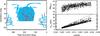 |
Fig. 1 Left panel: the footprint on the sky of our search in the DR7 CAS (light blue) and the distribution of the 939 galaxies constituting the CALIFA mother sample (red circles). Right panels: redshifts vs. absolute magnitudes Mr,GC (top) and r-band linear isophotal sizes (bottom) for the galaxies in the sample. The dotted lines in the lower panel are the selection limits. |
2. The CALIFA mother sample
In order to maintain flexibility in scheduling, the pool of galaxies available for observations in the CALIFA survey is somewhat larger than the expected number of total observations. This pool – henceforth called the CALIFA “mother sample” (MS) – is defined by the selection criteria detailed below. Galaxies are drawn from this pool for observation according to visibility alone, which should be close to random selection. At any given time, the set of actually observed CALIFA galaxies will therefore be a random subset of the MS. In the following we always refer to this MS when speaking about CALIFA galaxies, unless explicitly stated otherwise.
2.1. Selection of the mother sample
There were five main steps in the selection of the MS:
-
1.
Size selection: the MS was selected from the SDSS DR7(Abazajian et al. 2009). InCALIFA we are interested in nearby, bright galaxies. The SDSSspectroscopic sample suffers from incompleteness for objectsbrighter than an apparent magnitude of 14.5in r. We therefore started with the PhotoObjAll catalogue of DR7 and selected objects that have 45′′ < isoAr < 79.2′′. Here isoAr is the isophote major axis at 25 mag per square arcsecond in the r band1.
-
2.
Quality assurance cuts: we additionally applied cuts to avoid photometry problems as follows: a cut in Galactic latitude to exclude the Galactic plane: b > 20° or b < −20°; a selection on a number of flags (NOPETRO = 0, MANYPETRO = 0, TOO_FEW_GOOD_DETECTIONS = 0) to exclude obvious problems in the detections; a flux limit of petroMagr < 20 to exclude very faint objects. This yielded a sample of 1495 objects.
-
3.
Redshifts: we then downloaded properties for all 1495 objects from SIMBAD2. We used the “cz” redshifts when none were available from SDSS. For wavelength coverage reasons we restricted to redshift range to 0.005 < z < 0.03. This discarded objects that were actually stars, but also those that had neither SIMBAD nor SDSS redshift.
-
4.
Visibility: finally, to reduce problems due to differential atmospheric refraction, it is best to keep the airmass X < 1.5. The further limitation of hour angle to −2 h < HA < 2 h (to cope with PMAS flexure problems) then limits the declination to δ > 7 deg. Due to the sparsity of galaxies in the SDSS Southern area, this limit was only applied in the main SDSS area, i.e. for Right Ascension 5 h < α < 20 h.
-
5.
Final adjustments: of the nearly final sample of 942 objects, five were eliminated based on visual inspection (e.g. because they were part of a much larger galaxy that was shredded by the SDSS pipeline). Two objects were added later on by hand. One is NGC 4676B, the second system of the Mice galaxies. This object was added because the other object in the pair falls in our MS. This gave us the opportunity to study a merger system and to relate its properties to the larger sample. Also, it would in principle fit our size criteria, if it had been treated properly by the SDSS pipeline. The other object, NGC 5947, was observed due to a glitch with the database on the very first observing night. It however has properties very similar to objects in our main sample, so we left it in. To obtain a sample with the exact statistical properties described here, one would thus have to discard NGC 4676B and NGC 5947.
Within our final sky area there are only 18 objects which would have passed all our quality and size cuts but still have no redshift (942 have redshifts). Those objects are not part of the sample. This means that we are missing less than 2% of our sample, even if all of these were at the right redshift. In the more likely case that their redshift distribution is similar to that of those galaxies with redshifts, we are missing 1.2% of our sample.
The final CALIFA MS that we describe in this paper thus contains 939 objects. The final observed sample will be a random sub-selection of the MS in all physical galaxy properties. Sub-selection happens according to visibility only. The sky and redshift distribution of the MS is shown in Fig. 1. Note that absolute magnitudes in Fig. 1 are based on the analysis presented later in Sect. 6.3, which includes growth curve photometry of the CALIFA MS galaxies, hence the notation Mr,GC. These absolute magnitudes have been corrected for foreground (Galactic) reddening, but not for internal attenuation. Absolute magnitudes based on SDSS Petrosian magnitudes and redshifts only will be used on the following as well for purposes of comparison to a bigger SDSS sample. For these we use the notation Mr,p.
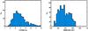 |
Fig. 2 Left: histogram of radial coverages of the CALIFA galaxies, i.e. the ratio between the radius of the Field of View of PPak and petroR50r. This figure does not give the actual spectroscopic coverage, which may be smaller due to S/N issues. Right: histogram of spatial scales with which the CALIFA galaxies are observed. A fibre diameter is 2.7′′, whereas the typical fibre-to-fibre distance is 3′′. The final spatial resolution of CALIFA will depend on future optimizations of the cubing code, but will be approximately 3′′. |
2.2. Distances, spatial coverage of the IFU and linear scale
Distances for the MS have been obtained from NED and Hyperleda (Paturel et al. 2003). From NED we retrieved the distances as corrected for Virgo, Shapley and Great Attractor infall, (Mould et al. 2000, in which H0 = 71 km s-1 Mpc-1, which is so close to our fiducial value that we do not correct for the difference). We also retrieved redshift independent distances from NED. Hyperleda makes available distance moduli which are corrected for Virgo-centric infall and we also derived distances from pure Hubble flow for comparison. Unfortunately, redshift independent distances do not exist for all our galaxies. Also, they are inhomogeneous, sometimes significantly so. We therefore use them as a benchmark only. The best correlation with redshift independent distances was found for the NED-infall-corrected ones, which are available for all galaxies. We therefore adopted those as our fiducial distances.
CALIFA was designed to cover “galaxies over their entire optical extent” and it is useful to verify how much this is the case. Figure 2 therefore shows the histogram of radial coverage in units of the SDSS pipeline quantity petroR50r, called r50 hereafter. Clearly, the overwhelming majority of our galaxies (97%) are covered to more than 2 × r503. In most cases we indeed obtain useful data out to these large radii. The real depth of CALIFA data is described in detail in Sánchez et al. (2012a) and Husemann et al. (2013). On average over the MS, the PPak IFU covers 1.4 times the isophotal diameter determined from the SDSS imaging, with the maximum and minimum values being 1.64 and 0.94, as per selection.
Another useful number is the average spatial scale of the CALIFA data, also shown in Fig. 2. The mean physical scale of one PPak fibre for the CALIFA MS is 1 kpc. The actual spatial resolution in the final data cubes delivered by CALIFA depends on the cube reconstruction software, which is still being optimized at the time of writing of this paper. Due to the three point dither pattern, we expect the final spatial resolution to be better than 1 kpc in the mean and better than 1.9 kpc for all galaxies in the CALIFA sample. CALIFA objects can thus not only be resolved in their different galaxy components (nucleus, bulge, disc, spiral arms), but due to the average distance between H II regions, even single H II complexes can be identified and studied (Sánchez et al. 2012b). Note that the redshift dependence of the size cuts in physical units and the intrinsic change of spatial resolution with redshift introduces a mass dependence of the spatial resolution as measured in kpc. This effect is approximately a factor of two between the highest and lowest redshift limits, but may still be important for some science applications.
2.3. Multi-wavelength data available for the CALIFA sample
We have cross-correlated the positions of CALIFA galaxies with those in a variety of available databases covering many wavelength ranges. Table 1 indicates the number of CALIFA galaxies which have a match in each survey. Whether consistent integrated fluxes are available (yet) is another question. We derived optical fluxes for CALIFA galaxies from a growth curve analysis in Sect. 6.1. To obtain matched integrated fluxes from the other surveys by growth curve analysis would be prohibitive and not necessarily useful, due to the different depth and background characteristics. We therefore suggest to resort to either using catalogues that represent “total fluxes” as derived by these surveys, or to determine own fluxes based on the apertures defined by the isophotal position angle, axis ratio and half-light major axis derived by the growth curve analysis.
The photometry used in Sect. 6.3 was derived from the following resources:
-
2MASS photometry: the CALIFA MS table was cross-matchedwith the 2MASS All-Sky Extended SourceCatalog (XSC) catalogue (Jarrettet al. 2000),providing J, H, Ks photometry in Vega magnitudes. These were converted to AB magnitudes using offsets of 0.91, 1.39, 1.85, respectively (Blanton et al. 2005a). The CALIFA galaxy coordinates were used to find extended 2MASS source entries within 20′′. For some galaxies the 2MASS coordinates can be significantly offset from the galaxy center by more than 10′′. Such cases were deemed unreliable and were not used in the final match.
-
GALEX photometry: the CALIFA MS table was cross-matched with the GALEX GR6 database (using the GALEXView tool) for all GALEX “tiles” that have their centers within 0.55 degrees of a CALIFA galaxy. The magnitudes were determined from a growth curve analysis and should therefore be equivalent to the optical magnitudes. The photometry was computed following the recipes in Gil de Paz et al. (2007). The total number of galaxies observed is 663 and the total number of galaxies where we have useful photometry is 655. There are no FUV data for 52 of the 655 galaxies, either because the exposure time in the FUV is not sufficient, or because the galaxy is extremely red. More details on the UV photometry will be contained in a forthcoming paper (Catalán-Torrecilla, in prep.).
3. How CALIFA compares to the general galaxy population
Available ancillary data.
The CALIFA survey was launched with the intention to characterize typical galaxies over a wide range of properties. This is in contrast to the samples of the SAURON project (de Zeeuw et al. 2002) and the ATLAS3D survey (Cappellari et al. 2011), which are focussed on early-type galaxies. Although some focussed projects using IFS on late type galaxies also exist (Ganda et al. 2006; Bershady et al. 2010), no existing survey using IFS has attempted to observe a sample of galaxies covering all types of galaxies.
We already demonstrated in Sánchez et al. (2012a) that the CALIFA MS covers the full area occupied by galaxies in the colour–magnitude diagram. In the following we address the issue of representation in a more rigorous way. We investigate which selection effects might be affecting the CALIFA sample, and we estimate the limits of representativity, outside of which the survey will not constrain the properties of galaxies in general.
3.1. Comparison data
The current state of the art for low-redshift galaxy surveys is set by the spectroscopic part of the SDSS (Strauss et al. 2002), which has enabled extensive investigations of galaxy properties in the nearby Universe. It is therefore natural to compare the statistical properties of the CALIFA MS with those of much bigger and well-groomed SDSS galaxy samples. Note that since CALIFA is based entirely on the SDSS photometric database, any fundamental limitations in those data (such as the well-known bias against very low surface brightness galaxies) will translate directly into corresponding selection effects for CALIFA. We do not discuss such effects further, but refer the interested reader to Kniazev et al. (2004).
Our comparison sample of galaxies extracted from the SDSS DR7 spectroscopic database is flux-limited to petroMagr < 17.7 and covers a geometric footprint in the sky of 8033 deg2, very similar to (but slightly less than) the CALIFA footprint. We considered only galaxies with well-measured SDSS redshifts between z = 0.003 and z = 0.1; there are some 260 000 galaxies matching this selection. For brevity, we denominate this set as “the SDSS sample” henceforth. For some of the tests presented below we further limited the outer redshift cut to the same value as for CALIFA, z < 0.03, which reduced the sample to 26 900 galaxies; this we call “the low-z SDSS subsample”. All relevant pipeline quantities such as apparent magnitudes, angular size estimates etc. are by construction consistent with those in the CALIFA tables, enabling direct comparisons. Note however that most of the SDSS galaxies are not only much fainter than the galaxies in CALIFA but also much smaller (in angular sizes), typically subtending no more than a few arcsec in the sky. This may lead to subtle systematic differences in some of the photometric quantities, due to the way the SDSS pipeline treats extended objects of different sizes, which ultimately limit the accuracy of this comparison.
3.2. Limits of the CALIFA selection
We first investigate the question that users of public data from the CALIFA survey might find most relevant: What are the ranges in absolute magnitudes, stellar masses, and linear sizes (half-light radii) over which CALIFA provides a representative sample? How sudden or gradual is the transition when moving away from this range? And in particular, are there domains where CALIFA has a complicated selection function, for example where only the most compact or the most extended galaxies are included in the sample?
Under the assumption that the SDSS sample is a fair representation of galaxies in the local Universe, these questions can be empirically addressed by applying the CALIFA size selection criteria to SDSS galaxies. When doing this it is important to realize that whether or not a galaxy is in CALIFA depends only on its linear isophotal size Diso and on its redshift. While most SDSS galaxies have angular sizes much too small for CALIFA, many of them have Diso values that at some other (generally lower) redshift would make them accessible to the CALIFA criteria. Only galaxies with Diso smaller than the smallest possible size Diso,min = 4.7 kpc – corresponding to isoAr = 45′′ at z = 0.005 – would not make it into CALIFA at any redshift. Equally, the maximum possible linear size of any CALIFA galaxy corresponds to  at z = 0.03, or Diso,max = 46 kpc.
In Fig. 3 we plot absolute magnitudes Mr,p against linear sizes Diso for both the SDSS and the CALIFA samples. For consistency between both samples, absolute magnitudes in this figure have been derived from the apparent Petrosian r band magnitude as given by the SDSS photometric pipeline and distances have been calculated directly from the observed redshift (i.e. neglecting any corrections for peculiar velocities of the galaxies). All SDSS galaxies within the two vertical dashed lines, i.e. within the range 4.7 kpc < Diso < 46 kpc, could and would be selected by CALIFA if located at a suitable redshift. For magnitudes −19 ≳ Mr,p ≳ −23, essentially all SDSS galaxies are within this domain, irrespective of their actual sizes. We quantify this by marginalizing over Diso and computing the fraction of SDSS galaxies within the CALIFA “accessible range”; this is shown in Fig. 4 (with Poissonian error bars representing the number of SDSS galaxies in each bin). The fraction is above 95% for the range 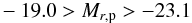 (1)and falls rapidly outside of that range. Notice that even the huge z < 0.1 SDSS sample contains only relatively few galaxies at Mr,p < −23, so that the error bars are correspondingly large.
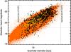 |
Fig. 3 Selection limits of CALIFA: absolute magnitudes Mr,p are plotted against linear isophotal sizes of galaxies in the CALIFA MS (black points), compared to the same for galaxies in SDSS (orange). The two vertical dashed lines delineate the range of galaxies accessible to CALIFA; all galaxies within this range would be selected by CALIFA if located at a suitable redshift. The horizontal lines represent the limits inside which for a certain luminosity bin the fraction of SDSS galaxies within the CALIFA “accessible range” is above 95%. |
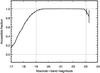 |
Fig. 4 Fraction of SDSS galaxies within the CALIFA accessible range of Diso, as a function of absolute magnitude. Error bars are Poissonian. The two vertical lines bracket the range where the fraction is >95%. |
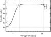 |
Fig. 5 As Fig. 4, but showing the fraction as a function of half-light radius (i.e. SDSS pipeline r50). The two vertical lines again bracket the range where the fraction is >95%. |
Since Diso is also correlated with half-light radius, we can perform the same exercise to determine the completeness with respect to that quantity. In Fig. 5 we show the marginalised fraction of SDSS galaxies within the CALIFA accessible range of Diso, now as a function of r50. The “accessible fraction” is again higher than 95% for the interval  (2)We finally also estimated the corresponding limits in stellar masses, anticipating the results from Sect. 6. We find that the fraction is above 95% for the range
  (3)Only outside of these “completeness limits” does the CALIFA selection function depend on galaxy size in a non-trivial way, in the sense that low-luminosity galaxies can get into CALIFA only if they have a large value of Diso (see also Sect. 5), and very high-luminosity galaxies may be captured in CALIFA only if they are abnormally small. However, less than 10% of all galaxies in the CALIFA MS are located in these “outside” regions of parameter space, most of them forming the low-luminosity and low-mass tail of the sample. For statistical purposes they should be left out of consideration.
Of course, only very few of the SDSS galaxies actually made it into the CALIFA sample; most are at too high redshifts and appear therefore as too small. But as long as the isophotal size distribution function is the same everywhere, this selection can be accurately quantified in terms of the formal survey volumes for CALIFA and SDSS, which we discuss in the next subsection. We thus conclude that for the given range in luminosities and masses, the apparent diameter selection does not introduce any size bias.
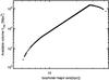 |
Fig. 6 Available survey volume for all galaxies in the CALIFA MS, as a function of linear isophotal size as derived from the observed redshift. |
4. Volume corrections and galaxy number density distributions
4.1. CALIFA survey volume
The CALIFA footprint on the sky subtends ΩC = 8700 deg2, see also Fig. 1. Together with the sample redshift range of 0.005 <z < 0.03, this converts into a formal comoving volume of ~1.7 × 10⁶ Mpc3 (adopting the cosmological parameters specified in Sect. 1). This, however, is not the actually available volume for the galaxies in the survey: Because of the narrow range in permitted angular sizes (less than a factor of 2), any galaxy of given linear size is included in the CALIFA selection only over an object-dependent range in redshifts (see Fig. 1).
The available volume per galaxy can be computed with the Vmax method by Schmidt (1968), the application of which is straightforward for a diameter-limited sample (e.g., de Jong & van der Kruit 1994). For CALIFA we assumed that the ratio between apparent and linear isophotal size of a galaxy depends only on its angular diameter distance (i.e. we neglected cosmological surface brightness dimming, and any “K correction in size”). We furthermore assumed pure Hubble flow distances, which should be a good approximation for most objects in the sample but may introduce distance errors of up to ~20% for the lowest redshift galaxies. We then computed, for each galaxy in turn, the minimum and maximum redshifts for which an object of the same linear size Diso would still be captured by the CALIFA selection criteria. The available volume Vmax follows directly from these object-specific redshift limits and the survey solid angle. It is easy to see that Vmax depends only on the value of Diso of a galaxy. Figure 6 shows the variation of Vmax with Diso for the CALIFA MS. The maximum volume of 1.5 × 10⁶ Mpc3 is reached for big galaxies located somewhat below the outer redshift boundary, while smaller (and therefore less luminous but more numerous) galaxies have much lower Vmax values.
These numbers are applicable to the full MS. At any given time, only a fraction fgal < 1 of all galaxies in that sample will have IFU data. Assuming that the observed objects constitute a random subset of the MS, this reduction can be condensed into an “effective solid angle” Ωeff = f × ΩC, and thus the value of Ω computed for the mother sample simply has to be corrected by the same factor fgal, which again translates into correcting downwards the Vmax values of each galaxy downwards by the same factor.
Before turning to apply these volume corrections to the CALIFA sample we have to take another effect into account, namely variations in the galaxy number density due to large-scale structure. These variations are significant even when averaging over ~106 Mpc3. We obtained a quantitative estimate of the magnitude of the effect on the CALIFA survey volume by the following procedure: We subdivided the SDSS comparison sample into redshift bins of Δz = 0.002 and counted the number of galaxies per bin. We then calculated, in each bin, the total number of galaxies expected from the Schechter fit to the “local cosmic mean” luminosity function by Blanton et al. (2003), taking into account the apparent magnitude limit of the SDSS spectroscopic sample and “evolving” the luminosity function from z = 0.1 to the mean redshift of each bin. The ratio of these two numbers provides an estimate for the redshift-dependent deviation of the number density of galaxies from the cosmic mean, averaged over scales corresponding to Δz = 0.002 and the SDSS DR7 footprint. The result is displayed in Fig. 7, showing that the variations amount to more than a factor of 2 between minimum and maximum redshift, for the CALIFA redshift range of z < 0.03. We note that a conceptually similar plot was already shown by Blanton et al. (2005b) only for the much smaller DR2 footprint and using infall-corrected redshift distances rather than plain redshifts.
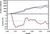 |
Fig. 7 Top: observed (black) and predicted (blue) number of SDSS galaxies with magnitudes r < 17.7 per Δz = 0.002 redshift bin. Bottom: ratio of these two numbers, as a function of redshift. |
We can now use these ratios to apply redshift-dependent correction factors to the galaxy number density. Doing so however implies a number of simplifying assumptions: (1) We neglect the differences in footprints between SDSS-DR7 (spectroscopic sample) and CALIFA. (2) We consider only variations as a function of redshift and neglect transverse effects. (3) We assume that the shape of the LF is always the same, only the normalization varies. Applying the correction is simple: If at the redshift z of galaxy X the relative under- or overdensity is δ(z), we give galaxy X a weight 1/δ. Mathematically this is equivalent to combining the inverse volume Vmax and the density factor δ into a single volume weight  and then use
  for all volume corrections. We demonstrate the relevance of this correction in the next subsection.
We thus conclude that the CALIFA MS is a statistically well-defined subset of the local galaxy population, with easily computable and quite accurately known volume weight factors per galaxy. It is important to keep in mind that any mean values computed directly from the observed sample (i.e. not corrected for survey volume) will be different from those of any other sample. In the next subsection we use these weights to explore how well CALIFA represents the mix of different galaxy types in the local Universe.
4.2. Luminosity function
We now investigate whether the overall number density of galaxies estimated from the CALIFA diameter-selected sample is in line with expectations from other surveys, thus whether or not CALIFA might be missing a significant fraction of galaxies. We also consider if galaxies of different luminosities are represented in adequate proportions by the sample.
To this purpose we constructed the binned r band luminosity function (LF) from the CALIFA MS using the Vmax estimator and compared it with the LF estimated from SDSS. While there are more sophisticated methods available for measuring luminosity functions, we are mainly interested in a global comparison for which the simple Vmax approach is sufficient. For the same reason we also did not attempt to apply any corrections for photometric incompleteness which would affect SDSS and CALIFA equally. We computed space densities both with and without the redshift-dependent correction for large-scale structure derived in the previous subsection. We did not apply k-corrections for this exercise, as these are very small for the redshift range considered.
For comparison we again used the Schechter function fit to the LF constructed from almost 150 000 SDSS galaxies by Blanton et al. (2003), adjusted to our cosmology and “evolving” the LF from z = 0.1 to the mean redshift of the CALIFA sample. The outcome of this comparison is shown in Fig. 8, demonstrating that CALIFA allows us to estimate the galaxy number density and luminosity function for absolute magnitudes Mr,p < −18.6 with reasonable fidelity.
While the LF computed from the CALIFA sample without density correction (shown as orange squares in Fig. 8) is already quite close to the one from SDSS, the differences in some points are certainly greater than the Poissonian error bars. However, an accurate match would be purely fortuitous given the significant redshift-dependent modulations in galaxy number density shown in Fig. 7. But when we apply the redshift-dependent correction (i.e. using the effective volume weights defined above), the agreement becomes almost perfect. Recall that while the correction is applied to the CALIFA sample, it was derived from the full SDSS sample alone without any reference to CALIFA. It is remarkable that both the overall normalization and the relative distribution of luminosities are captured so well by the CALIFA sample, given that it comprises less than 1000 galaxies.
At luminosities below Mr,p ≈ −18.6, the LF from CALIFA turns over and stays below the SDSS LF. This indicates the expected incompleteness at low luminosities, which in turn is a direct consequence of the low-redshift limit of CALIFA that excludes dwarf galaxies with Diso < 4.6 kpc. While there is also a related high-luminosity completeness limit at Mr,p,min = −23.1 due to the upper redshift cut, this limit is actually washed out by small number statistics: According to the luminosity function, the number density of galaxies at Mr,p = −23 is approximately 10-6 Mpc-3, which in combination with the maximum survey volume (Fig. 6) implies that the total number of such galaxies expected for CALIFA is of order unity. In other words, galaxies more luminous than Mr,p = −23 might be missing if they are too extended, but already independently of size they are largely absent in CALIFA because the survey volume is too small.
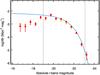 |
Fig. 8 The red points show the r band luminosity function of galaxies estimated from the CALIFA MS, using absolute magnitudes from the SDSS Mr,p and with error bars representing Poissonian uncertainties only. The orange squares are for the same sample, but without the corrections for variations in cosmic density. The blue solid line shows the Schechter fit to the LF of Blanton et al. (2003), adjusted to our cosmology and redshift range. The vertical dashed lines indicate the completeness limits derived in Sect. 3.2. The faintest magnitude at which the luminosity function itself is marginally consistent with that of Blanton et al. would imply that the limit of completeness for the CALIFA sample is at roughly Mr,p < −18.6. |
These comparisons demonstrate that in terms of total number density and the distribution of luminosities, the CALIFA MS is very close to a fair representation of non-dwarf galaxies in the local Universe.
4.3. Size distribution function
A distribution related to the LF is the size distribution function (SDF), quantifying the differential number density of galaxies at a given linear size. We use here the isophotal sizes Diso and construct a binned estimate of the SDF in the same way as the LF. The result is depicted in Fig. 9, again with redshift-dependent number density correction, together with the SDF determined by us from the SDSS low-z subsample. Notice that the number density φ is given here per logarithmic decade.
The agreement is again satisfactory, especially after density correction. This plot also shows (more clearly than in the LF) that CALIFA as a sample covering only a small range of apparent sizes reacts differently to large scale structure than a survey with a one-sided flux-limit. Consider the CALIFA points at log (Diso/ kpc) ~ 1.1. When uncorrected, these points deviate most strongly from the SDSS-based SDF. Figure 1 shows that galaxies with these sizes in CALIFA are located at redshifts around and just below z ≈ 0.015, where the underdensity in the local Universe happens to be most pronounced (see Fig. 7). Galaxies located there will be too rare in the sample compared to the cosmic mean. Thus, large-scale structure affects the shape of the resulting distribution function from CALIFA, whereas for a sample with a one-sided flux limit it mainly modulates the overall normalization. In both cases it is of course possible to correct for such effects, provided that the variations as a function of redshift are known.
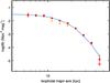 |
Fig. 9 Distribution function of linear isophotal sizes Diso of galaxies estimated from the CALIFA sample, compared to the same distribution constructed by us from the SDSS low-z subsample. Symbols and line types as in Fig. 8. |
5. The faint limit of the sample and the axis ratio distribution
We now come to a property where we expect noticeable selection effects. It is long known that isophotal sizes of flattened, transparent (no attenuation) galaxies vary with inclination, simply due to the projected change of surface brightness (e.g., Öpik 1923). It is therefore easier for an inclined disc galaxy to get into a sample defined by a minimum apparent isophotal size than it is for a face-on system of the same intrinsic dimensions. The magnitude of this effect depends on the degree of transparency; it is strongest for a fully transparent galaxy, and it disappears when the system is opaque, so that only its surface is observed. Notice that exactly the opposite selection effect exists for flux-limited surveys, favouring face-on systems over inclined ones. In this case the effect is significant when extinction is large, while it is negligible for transparent galaxies.
Yet, inclination is not an easily measurable quantity. For highly flattened (disc-dominated) systems the ratio between minor and major photometric axes can be used as a proxy. We thus expect that the CALIFA sample might display an excess of galaxies with low axis ratios, at least among disc-dominated systems, compared to a volume-limited sample. Such a dataset was constructed based on the SDSS by Maller et al. (2009, hereafter M09), with the explicit purpose to statistically constrain the intrinsic shapes of galaxies. Axis ratios from the 2nd order moments of the light distribution were obtained in Sect. 6. Moment based axis ratios give similar results as those obtained from fitting Sérsic models to the surface brightness distribution of galaxies, thus they provide a fair comparison to the results of M09.
In Fig. 10 we show the overall histogram of light-weighted axis ratios of the CALIFA MS, which turns out to be almost flat. Since any inclination-dependent selection effects should be most clearly seen for intrinsically flat disc-dominated galaxies, we separated the MS into early and late types by their concentration indices c ≡ r90/r50 in the r band, with the dividing value at c = 2.6 (e.g., Strateva et al. 2001; Lackner & Gunn 2012). Figure 10 also shows the axis ratio distribution of only the c < 2.6 (=disc-dominated) galaxies, additionally limited to absolute magnitudes Mr,p brighter than −18.6 (cf. Sect. 3.2). For comparison the corresponding distribution of low Sérsic index (n < 1.2) galaxies from the approximately volume-limited sample of M09 is also plotted, rescaled to match the corresponding number in the CALIFA sample. These two histograms are apparently very similar, indicating that the selection method for CALIFA does not strongly bias the axis ratio distribution of luminous disc galaxies in the sample.
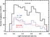 |
Fig. 10 Histogram of axis ratios (2nd order moments of the r band light distribution) for the CALIFA MS. Overplotted in blue is the histogram for disc-dominated systems with Mr,p < −18.6 and concentration indices c < 2.6, and in red for comparison the axis ratio distribution (rescaled to the same number of objects) for the disc-dominated galaxies in the SDSS sample of Maller et al. (2009). |
We caution that light moment based axis ratios are weighted by light and thus are more sensitive to the brightest parts of a galaxy. Especially in presence of bulges, they tend to underestimate the axial ratio of the disc component, which is instead well represented by the outer isophotes. We therefore also considered the alternative approach of using the SDSS photometric pipeline delivered isophotal major and minor axes (isoAr and isoBr) that can be combined into an axis ratio at the outer 25 mag/arcsec2 level. The histogram of isophotal axis ratios in Fig. 11 is now clearly skewed towards low values of b/a, providing some indication for the above selection effect in the CALIFA sample. To understand this better, we show as dotted histogram (in red) in Fig. 11 the 55 galaxies of the CALIFA MS with Mr > −18.6, thus below the completeness limit. Nearly all of these have axis ratios below 0.4 (this remains true when taking light-weighted axis ratios instead); visual inspection of the images confirms that these are predominantly disc-dominated systems seen close to edge-on. Presumably very few of these galaxies (if any) would have made it into the CALIFA sample if seen face-on; their angular sizes have been boosted through inclination, just enough to elevate them into the sample. We note in passing that in our flux-limited SDSS comparison sample we can directly verify the opposite trend mentioned above, namely that the distribution of isophotal axis ratios is skewed towards larger values. This is a direct consequence of non-negligible extinction in the r band acting on highly inclined systems (e.g. Disney et al. 1989; Boselli & Gavazzi 1994; Unterborn & Ryden 2008; Padilla & Strauss 2008).
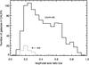 |
Fig. 11 Histogram of isophotal axis ratios (at 25 mag/arcsec2 level) for the CALIFA MS. Overplotted with a dotted line is the histogram for the 55 low-luminosity systems with Mr,p > −18.6, which are almost all highly inclined disc systems. |
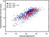 |
Fig. 12 Relation between absolute magnitudes (Mr,p, uncorrected for internal extinction) and linear isophotal sizes of the CALIFA MS, colour–coded according to isophotal axis ratios. |
Figure 12 shows how inclination increases the isophotal sizes and weakens the magnitudes of disc-dominated galaxies, leading to a widening of the apparent luminosity-size relation. Take two galaxies with the same intrinsic size and luminosity, one seen face-on, one edge-on. While the face-on galaxy will be seen at its original position within the size-luminosity relation, the one seen edge-on will be shifted towards fainter magnitudes and larger isophotal major axis, i.e. perpendicular to the size-luminosity relation itself. The exact mix of internal extinction and surface brightness boosting due to inclination will depend on the galaxy type and thus presumably also on luminosity and mass. We make no attempt here to disentangle the two effects.
While the CALIFA sample thus has a higher proportion of inclined disc galaxies at the faint end, the overall effect is not large. When using a light-weighted estimate of axis ratios, there is in fact no significant difference to the volume-limited sample of M09; when adopting axis ratios measured at an outer isophote the effect becomes more noticeable. Specifically for the galaxies close to and below the low-luminosity completeness limit there is at any rate a clear surplus of galaxies with very high inclinations in the CALIFA sample.
We finally note that the ability to perform volume corrections for the CALIFA sample is completely unaffected by this possible selection bias for inclined galaxies. For any given galaxy, the available volume Vmax depends only on its observed size and on its redshift; moving a galaxy in- or outwards until it leaves the sample selection corridor has obviously no consequence for its inclination.
6. Photometry, morphology, and stellar masses
The SDSS pipeline has been optimized for a large survey and it was clear from the outset that the catalogued photometric properties for our sample would have to be verified. In particular, the CALIFA MS galaxies are bigger on the sky than the objects the SDSS pipeline has been optimized for. The SDSS pipeline Petrosian fluxes for the CALIFA MS therefore are likely to be affected in a different way than for a typical, large SDSS sample in the sense that their fluxes will be biased even lower as compared to the usual offset between the likely total flux from the galaxy and the Petrosian flux. We therefore set out to produce photometric quantities attempting to sum up all the available flux per galaxy using our own analysis. The reader should bear in mind that biases in comparisons between different samples will arise if the techniques used to obtain the photometry differ strongly.
6.1. Growth curve analysis
The first step to obtain reliable integrated photometry from the images was to produce growth curve (GC) photometry for all sample galaxies in all bands. We used images from DR7. We first constructed masks for bright stars and background galaxies. In a first pass, masks were produced from the segmentation image of SExtractor (Bertin & Arnouts 1996). These were then extended by hand for the regions within the galaxies, as SExtractor is not able to reliably identify foreground objects within galaxies. Neglecting the flux from masked regions would have led to systematic underestimation of galaxy brightness. In order to evaluate and include the missing flux from masked areas, we interpolated the masked regions using an inverse-distance weighted average. In order to apply the masks (corresponding to r band images) to all 5 SDSS bands, we measured the shift between the different images and their r-band counterparts using their WCS (FITS World Coordinate System) RA and Dec coordinates, then shifted and cropped the masks accordingly. Inspecting the masked images visually, one sees that some light still spills out from rectangular masked regions, and some faint stars are left unmasked as well. While this would mean that the “real” sky flux is systematically overestimated, our galaxies are extended so it is likely that they also contain such unmasked foreground objects.
The position angle (PAgc) and axis ratio (b/agc) values were obtained by calculating light moments (see Sect. 10.1.5 of the SExtractor manual vs. 2.13 and Bertin & Arnouts 1996). The final b/agc value is the mean of the axis ratios of ellipses containing 50% and 90% of the total flux. This is motivated as a compromise between a correct representation for most of the light (and thus correct derivation of the half light major axis) and a correct representation of the galaxy outskirts (and thus correct derivation of the total light).
To derive the actual growth curve, all pixels on ellipses with successively incremented major axes and with fixed b/a and PA were summed up. If we were fitting the flux profile in sufficiently wide rings using simple linear regression, the best fit line should become horizontal at some radius, which we might then consider to be the edge of the galaxy. This statement would assume that galaxy flux falls off asymptotically until it is indistinguishable from the sky fluctuations. In practice this is not the case, given that incomplete masks, light from other objects and sky gradients make the best fit slope switch from negative to slightly positive at some point. We opted for a solution in which we fit 150 pixel wide sections of the flux profile using simple linear regression, with neighbouring fit sections overlapping by 100 pixels. When the flux profile slope becomes non-negative, we take the mean of the current ring as the sky value, and the ellipse with major axis value at the middle of the ring as the galaxy’s edge. We have verified that this procedure gives good results and is robust even in the presence of masked regions or faint unmasked objects. We added simulated de Vaucouleurs and exponential profiles to real sky backgrounds, including those with various defects, and ran the growth curve code on them. The procedure recovers practically 100% of the flux for both de Vaucouleurs and exponential profiles.
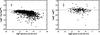 |
Fig. 13 Left panel: comparison of apparent magnitudes obtained from growth curve measurements with those from the SDSS pipeline (petroMagr). Right panel: comparison of apparent g magnitudes obtained from growth curve measurements with estimates of the same derived from the RC3. Both panels show typical error bars in the upper left corner. |
The determined sky is of course very important for extended objects such as our sample galaxies. We thus subtracted the sky from the images before constructing the growth curve. We verified that there are no significant differences between the sky measurements from the SDSS pipeline and from the growth curve routine.
The growth curve procedure was repeated with circular apertures for comparison purposes. The half-light major axes (HLMA, for elliptical apertures) and half-light radii (HLR, for circular apertures) were calculated once the total extent and flux of a galaxy were known. We use the difference between circular and elliptical growth curve magnitudes as an indication of the uncertainty on each magnitude. The standard deviation of this scatter is 0.14 mag. We find that the resulting magnitudes are indistinguishable in a systematic way. The same is not true for the HLR, which is highly dependent on the projected inclination. The HLMA depends less on inclination and we therefore consider it to be a better measurement of the true half-light radius of galaxies. We henceforth denote the HLMA as re to distinguish it from the r50 based on SDSS pipeline Petrosian fluxes. We will adopt growth curve measurements based on the elliptical annuli from here on.
6.2. Comparison of photometric measurements
It is instructive to compare the photometric measurements made in this section with the SDSS DR7 pipeline values as well as the values from the RC3 catalogue (de Vaucouleurs et al. 1991; Corwin et al. 1994). While our measurements are based on the same data as the DR7 pipeline values, they are more comparable to the RC3 values in terms of the method used to recover them.
The left panel of Fig. 13 shows this comparison between the r-band growth curve magnitudes and petroMagr from the SDSS pipeline. There is an overall correlation between the two quantities, which is satisfactory. But clearly, growth curve magnitudes are systematically brighter, and more so for bright galaxies. This is naturally explained by considering that GC magnitudes are meant to include all the flux of the galaxies, whereas Petrosian magnitudes have been defined to include a well-defined fraction of the total galaxy flux, as independent as possible of magnitude. The correlation of magnitude difference with absolute magnitude is due to the correlation of absolute magnitudes with morphological type and therefore Sérsic n in the CALIFA MS. Indeed, Blanton et al. (2001) show that Petrosian magnitudes contain between 82% and 100% of the flux for a de Vaucouleurs and exponential profile, respectively. The mean difference between the two measurements is Δ(mag) = 0.34 in the sense that growth curve magnitudes are brighter. For correction onto the CALIFA GC system, the offsets that have to be applied per SDSS magnitude intervals are: petroMagr > 14: −0.19, 14 > petroMagr > 13: −0.22, 13 > petroMagr > 12: −0.34, petroMagr < 12: −0.45. There are a few “catastrophic” outliers, which are due to shredding of large objects in the SDSS pipeline. Otherwise the scatter around the mean difference is 0.24 mag. Note that the uncertainty on the magnitudes of the CALIFA sample as determined by the SDSS pipeline is of 0.03 mag, which seems very low in light of this comparison.
There are 172 galaxies in common between the RC3 and the CALIFA MS that have RC3 total magnitudes. The right panel of Fig. 13 shows a comparison between the g-band growth curve magnitudes and an estimate of the g band magnitude determined from the RC3 using their B-band total magnitude and B −V colour as well as the following equation from Jordi et al. (2006):  (4)The mean offset between gGC and gRC3 is just −0.04 mag, with most of the offset due to very few outliers (the median difference is −0.01 mag). The scatter around the mean difference is 0.22 mag. The mean uncertainty on the RC3 magnitudes is 0.16 mag. Together with the 0.14 mag uncertainty on the growth curve measurements, this scatter thus seems mostly due to uncertainties in the determination of the total magnitude.
We conclude that reliable photometry of galaxies of the mother sample is now available in the form of these growth curve magnitudes. A systematic study of the dependence of flux recovery in the SDSS as a function of galaxy size on the sky and structural properties is, however, beyond the scope of the current paper.
6.3. Absolute magnitudes and stellar masses
To derive absolute magnitudes and stellar masses, one needs to determine the rest-frame SED of the galaxy and convolve it with the known filter response functions or multiply with the fitted mass-to-light ratio. Many assumptions and technical tricks go into these derivations (Walcher et al. 2011), and it is beyond the scope of this paper to describe in detail how these are addressed. We therefore calculated stellar masses using two existing and well-tested codes, namely kcorrect (Blanton & Roweis 2007) and an algorithm that has been extensively used and tested in Walcher et al. (2008, W08). Both codes rely on Bruzual & Charlot (2003) stellar population models with a Chabrier stellar initial mass function (Chabrier 2003), but the W08 code employs an unpublished updated version of the BC03 models, which is termed CB07 (see W08 for details). The codes differ notably in their assumptions about the underlying star formation histories, and in their routines to derive the best matching physical properties. In particular, the W08 code uses a Bayesian method to derive probability density functions for the output parameters, thereby allowing accurate determinations of uncertainties. Both codes sample wide ranges of star formation histories (with differences in the details) and dust attenuation amplitudes. We applied both codes only to the optical growth curve photometry. Stellar masses agree very well, with a systematic deviation of 0.1 dex in the sense that the W08 masses are lighter as expected due to the inclusion of secondary bursts in the library of star formation histories (see W08). The RMS scatter of 0.15 dex is nearly indistinguishable from the mean 1σ uncertainty of 0.11 dex calculated by the W08 code. Both codes are equally affected by IMF uncertainties, which may be of the same order as the quoted uncertainties. Owing to the slight differences between the kcorrect and the W08 masses, there does not seem to be a strong reason to prefer one over other, although the W08 masses could be more appropriate in those cases where the galaxies did experience recent bursts of star formation.
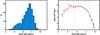 |
Fig. 14 Left panel: distribution of stellar masses in the CALIFA sample from a fit to the optical spectral energy distribution. Right panel: mass function of the CALIFA mother sample compared with the mass function from Moustakas et al. (2013). The two vertical lines indicate the representativity limits derived using the same method as in Sect. 3.2 from the low-z SDSS comparison sample: 9.65 < log (M⋆/M⊙) < 11.44. |
We also applied the W08 code to SEDs with added GALEX and 2MASS photometry (see Sect. 2.3) which provide a better constraint on the dust components. In cases where either in the UV or the NIR photometry data points were flagged as bad, these were not used and we reverted to simple optical masses. This makes the final catalogue somewhat inhomogeneous. Nevertheless, overall the derived masses are lower by 0.13 dex than the optical ones, with a scatter of 0.13 dex. Quoting from W08, “the mean ratios of masses determined without NIR data to the masses derived with NIR data are 2.8, 1.50, 1.0 for bins of specific star formation rate log (SSFR/yr-1) of [−16, −13] , [−13, −10] , [−10, −8], respectively”. This effect is thus expected. We adopt stellar masses based on the UV, optical and NIR SEDs from now on.
Figure 14 shows the derived stellar mass histogram. The CALIFA sample covers galaxies between 109 and 1011.5M⊙, with a sharp peak between 1010 and 2 × 10¹¹M⊙. This figure thus shows the range of stellar masses where the statistical power of CALIFA is best. Figure 14 also shows the mass function derived from these stellar masses and the volume corrections derived above and compares it with the mass function from Moustakas et al. (2013). The near perfect agreement over a large range of stellar masses shows the range of stellar masses where the CALIFA sample can be used to derive statements about the general galaxy population.
6.4. Morphological composition of the sample
One of the defining characteristics of the MS is that it contains galaxies of all morphological types. When looking through the morphological classifications available from public databases we found that these were incomplete for our sample (e.g. Galaxy Zoo 2, 535 matches Willett et al. 2013) or missing a consistent classification in Hubble subtypes (NED). We therefore undertook our own reclassification.
To obtain a morphological classification for the CALIFA galaxies we used human by-eye classification. Five co-authors classified all 939 galaxies in the MS according to the following criteria:
-
1.
E or S or I for elliptical, spiral, irregular;
-
2.
0–7 (for Es) or 0, 0a, a, ab, b, bc, c, cd, d, m (for S) or r (for I);
-
3.
B for barred, otherwise A. AB if unsure;
-
4.
Merger features, yes or no.
For mergers, Cols. 1 to 3 were filled with the properties of the main object, if possible. If nothing at all was possible U (unknown) was written there. The classifiers gave equal weight to SDSS postage stamps in r and i band.
The five tables obtained were combined, clipping outlier measurements in the calculation of the mean, but keeping them as minimum and/or maximum values. Figure 15 shows the resulting morphology histogram. We verify that the CALIFA MS covers a broad range in galaxy morphologies.
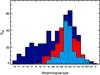 |
Fig. 15 Distribution of morphological types in the CALIFA sample from our own classification. Independent histograms are drawn by bar classification as non-barred (meanbar = A, full line, dark blue), strong bar (meanbar = B, dashed, blue) and weak bar (meanbar = AB, dotted, red). |
It may be of interest to note that 8 galaxies in the MS are classified as cD galaxies according to NED. These are (with cluster name when known): NGC 0731, NGC 1361, NGC 2832 (Abell 779), NGC 4556 (Tago 41262), NGC 4841A (Abell 1656, Coma), NGC 4874 (Abell 1656, Coma), NGC 5444 (Math 1280, 2MASS 845), NGC 6021 (Tago 71733).
Cross-correlation of CALIFA sample with literature catalogues.
Summary of the membership of the CALIFA sample to galaxy associations.
7. Environment
Environmental effects are expected to play a significant role in galaxy evolution. However, the many physical processes, their varying amplitudes and timescales make it observationally difficult to directly quantify the consequences. One of the difficulties is the challenge of defining a general measure of environment. In practice, different measures of environment will be relevant for different physical effects. With this in mind we decided to provide a range of estimations of environment in the present paper. Generally speaking, environmental measures differ by the size of the probed volume and by whether they concern themselves with structures in the galaxy distribution (e.g. isolated, pairs, groups, clusters, etc.) or whether they look at the mean density of galaxies on a given spatial scale. For a discussion of standard literature methods see e.g. Gavazzi et al. (2010). The primary aim of the present section is to verify whether we are lacking any particular kind of environment. Given our restricted sample size, the very general aim of this paper, and the difficulties of constructing appropriate comparison values, it would be pointless here to dissect the sample into subclasses for every environmental measure. This will be undertaken in dedicated papers and in relation to specific scientific goals.
7.1. Membership to well known structures
Galaxies aggregate into structures of very different sizes and scales: from isolation to massive clusters. Each scale has a different effect on the evolution of galaxies and no clear boundaries can be defined. For this reason we determined the membership of CALIFA galaxies to well known catalogues of galaxy aggregates, as one way to characterize their environment.
In a first step we determined the membership of CALIFA galaxies to catalogues of aggregates of a few galaxies, so that all the galaxies in a group are clearly identified: the AMIGA catalogue of isolated galaxies (Verdes-Montenegro et al. 2005), isolated pairs and triplets of galaxies (Karachentsev 1972; Karachentseva et al. 1987), and compact groups of galaxies (Hickson 1982). We also include in this list the Virgo Cluster Catalogue (VCC, Binggeli et al. 1985) with background source classification from the GOLDMine database (Gavazzi et al. 2003). Specifically, 3 of the 35 CALIFA galaxies in the Virgo Cluster Catalogue are classified as Virgo background galaxies in GOLDMine. Table 2 shows the result from a cross-correlation of the CALIFA sample with the catalogues listed above.
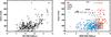 |
Fig. 16 Left panel: comparison between a pair of related environment measures. The mass of the host halo from the Wang et al. (2011) catalogue vs. the velocity dispersion of the closest known structure compiled in this work. Right panel: stellar mass distribution of members in known structures. The largest known structures have been identified. Galaxies have been colour coded by their morphological classification. |
As a second step we cross-correlated the CALIFA sample with the positions of compilations of loose groups and clusters found in the literature (White et al. 1997; Aguerri et al. 2007; Hernández-Fernández et al. 2012; Mahdavi & Geller 2001; Miller et al. 2005; Popesso et al. 2007; Shen et al. 2008; Garcia 1993; Mahtessian & Movsessian 2010; Tago et al. 2010; Crook et al. 2007; Mahdavi & Geller 2004; Berlind et al. 2006). In this case, as these aggregates of galaxies are defined by density peaks of galaxies in the spatial or radial velocity coordinates, the number of galaxies belonging to each aggregate is uncertain and in most cases the membership to a given aggregate is derived only for the most massive galaxies. A more natural way to ascertain the membership of a galaxy to an aggregate is a combination of its projected distance to the center and its relative radial velocity with respect to the systemic radial velocity of the aggregate.
Thus for each CALIFA galaxy we computed the projected distance to the center of all the groups/clusters in units of the virial radius. We adopted R200, computed following Finn et al. (2005), as a good estimate for the virial radius. We also obtained the differences in radial velocity with respect to those of the groups/clusters in units of the velocity dispersion. Table 3 contains the results of the cross-correlation of the CALIFA sample with the groups/clusters catalogues previously mentioned. The parameters va,σa describe the association, while vg refers to each galaxy. Dp is the projected distance on sky.
As a way to distinguish between the environments of CALIFA galaxies, we decided to separate them into galaxy aggregates with σ ≤ 550 km s-1 (hereafter LV associations), the less massive, and those with σ > 550 km s-1 (hereafter HV associations), the more massive and dense (Poggianti et al. 2006). Note that this separation is purely arbitrary and does not necessarily imply a scale of physical transformation. Indeed transformation of satellites may occur at lower σ and at Mhalo < 1013M⊙ (e.g. De Lucia et al. 2012). Given that we are dealing with a very large number of LV and HV associations and that a detailed dynamical analysis of all of them is out of the scope of this work, we present the number of CALIFA galaxies belonging to an LV/HV association following three different criteria which are usually found in the literature:
-
The number of galaxies that a projected dis-tance lower than the virial radius and with | vrad − vassoc | < σassoc of a given LV and HV galaxy association. This criterion identifies the members of the cluster core and does not take into account the members from the infall regions or rebounding members after a high velocity passage close to the cluster center.
-
The number of galaxies at a projected distance lower than the virial radius and with | vrad − vassoc | < 3 × σassoc of a given LV and HV galaxy association. This criterion includes some information about new infalling members but may include some foreground/background members especially close to the R200 border because of the relaxed 3 × σ condition.
-
The number of galaxies falling inside the average caustics proposed by Rines et al. (2003) for their sample of nearby clusters up to a projected distance of 5 × R200 from any LV or HV association. This criterion seems to be the most appropriate to determine the membership of a galaxy to a LV/HV association because it takes into account galaxies from infall regions and also rebounding galaxies. However deviations of the average caustics used in this work with respect to the true caustics could lead to incorrect assignments of the individual galaxies to LV or HV associations.
In summary, 246 galaxies likely belong to no known association, 567 likely belong to a low mass association and 126 likely belong to a high mass association. We conclude that we sample all types of group memberships within the CALIFA MS. The sky region covered by the survey includes well known structures such as the Coma/A1367 supercluster as well as isolated galaxies in the Great Wall. Concerning the Virgo cluster, the lower redshift cut at 1500 km s-1 implies that it is only partly covered by our survey. Virgo has a 3D structure with the main body at ≈1200 km s-1, but some subclusters further away (2000 km s-1, see e.g. Gavazzi et al. 1999). Figure 16 (right panel) shows the distribution of galaxies over stellar mass and velocity dispersion of their host structure, as well as their morphological type.
7.2. Halo mass catalogue
We matched the CALIFA MS with the group catalogue extracted from the SDSS DR7 by Wang et al. (2011) and Yang et al. (2007). This catalogue uses a group finder and SDSS DR7 to determine group membership and likely halo masses for SDSS galaxies. The matching was done by imposing that the angular distance between a CALIFA galaxy and a catalogue object be smaller than 1.5′′. This results in 513 CALIFA matched galaxies. The maximum angular distance is 1.1′′, and about 50% of the galaxies have angular distances ~0.1′′. Besides the mass of the parent halo, the matching also produces information on the group hierarchy: A rank of 1 indicates that the galaxy is a central galaxy (the most massive one of the group), while a rank = 2 labels the galaxy a satellite.
The CALIFA MS contains galaxies belonging to halo masses between 1011 and 1014 M⊙.
7.3. Local density of the CALIFA galaxies
The number density of local galaxies was computed using the projected comoving distance to the Nth nearest neighbour (dN) of the target galaxy. Thus, the projected galaxy density is defined as 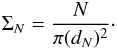 (5)We defined the nearest neighbours using two different samples. First, we select only those galaxies with spectroscopic redshift located in a velocity range of ±1000 km s-1 from the target galaxy and with a luminosity contrast of ±2 mag. These two constraints are similar to those used by Balogh et al. (2004a,b) and allow us to limit the contamination by background/foreground galaxies even if we are working with projected distances. Secondly, we defined a photometric sample and we select only those galaxies with photometric redshifts in the interval pz < zgal + 0.1 to account for the uncertainties in the photometric redshifts (e.g., see for a similar approach Baldry et al. 2006). To account for possible edge effects in our sample, we flagged those galaxies with dN greater than the distance to the edge of the survey, as these galaxies will have much more uncertain environmental densities.
We calculated the number density using the third, fifth, eighth, and tenth nearest neighbours, for both the spectroscopic and photometric samples. The last two measurements were averaged and the differences give us an indication of the uncertainties in the calculated densities (Baldry et al. 2006). The mean uncertainty in the same parameter over the sample is ≈1.4 galaxies/Mpc2. Another way of testing the accuracy of our densities is by comparing our different estimations based on the number of neighbours. We found a good agreement, with typical standard deviations of 0.3, 0.4, and 0.5 dex in the Σ3 − Σ5, Σ3 − Σ8, and Σ3 − Σ10 differences, respectively. Comparison of our values with those of Tempel et al. (2012) also shows good agreement. We thus conclude that the presented values are robust and eventual differences to other measurement methods will be due to physical differences between them.
For orientation, the density as computed from the 5th nearest neighbour varies between 0.1 and 55 galaxies per Mpc2 in our sample. Densities of Σ5 < 1 Mpc-2 correspond to very low-density environments, 10 Mpc-2 > Σ5 > 1 Mpc-2 correspond to loose groups, and Σ5 > 10 Mpc-2 correspond to compact galaxy groups and clusters (compare Aguerri et al. 2009). According to these criteria, 240 galaxies are located in low density environments, 387 in medium density and 310 in high density environments. We thus conclude that the CALIFA MS samples also all environmental densities.
7.4. Tidal forces
To characterize the influence of close neighbours on the CALIFA sample galaxies we followed the method by Varela et al. (2004). The Varela tidal perturbation f parameter measures the ratio between the internal forces (Fint) and external tidal forces (Fext) at the outskirts of a given galaxy, as caused by satellite/neighbouring galaxies. It does not take into account the relative velocities, as this information is not available for most of the non-CALIFA galaxies in the neighbourhood. Relative velocities may have an influence on the strength of observed features through the duration of the tidal encounter.
To determine f we searched for local neighbours of each CALIFA sample galaxy in the SDSS DR8. For robustness we only extracted galaxies with well determined magnitudes and Petrosian radii in the r and g band. For each galaxy the information is taken from the catalogues PhotoObj and SpecObj. The criteria to find the satellites were:
-
1.
Objects classified as galaxies (type = 3).
-
2.
Up to 200 kpc from the CALIFA target (assuming simple redshift-based radial and tangential distances).
-
3.
With reported values of Petrosian radii at 90% and at 50% flux in r and g bands. (acceptable values, we excluded objects with negative errors in the Petrosian radii).
-
4.
With sizes of at least 2 kpc (as provided by the petroRadr).
-
5.
With good quality flags [flagsr = 0 AND flagsg = 0].
We then calculated for all identified neighbours of a CALIFA galaxy the f parameter according to Varela et al. (2004), i.e. the tidal force exerted by the neighbour onto the CALIFA galaxy. Using mG and mP as the apparent magnitudes of the primary and perturber galaxies, respectively, R as the size of the galaxy and Dp as the projected distance between the galaxy and the perturber on the plane of the sky at the distance of the primary, the equation given by Varela et al. (2004) to calculate f is:  (6)Conceptually, an f value below −4.5 indicates no tidal influence, values between −4.5 and −2 indicate that there is weak influence at most and objects with an f value above −2 could be producing interaction effects on the CALIFA galaxy. From this environmental measure alone we would conclude that 335 galaxies in the CALIFA MS are completely isolated. On the other hand, there are 185 that could suffer from strong tidal effects. These numbers again confirm that the CALIFA sample is suitable for studying effects of galaxy interactions, while simultaneously providing a bona fide comparison sample of completely isolated galaxies.
7.5. Interactions
In this catalogue, our goal was to select from the MS those galaxies with evident signatures of interaction/merging (i.e., tails, bridges, rings, etc.). Three classifications were performed in total by different members of the collaboration with different scientific goals.
-
1.
The interaction flag described in Sect. 6.4.
-
2.
SDSS images were inspected for features indicating interaction. The unsharp masking technique was used. We use here a binary flag, lumping together all different morphological hints of interaction (streams, disc-disturbance, compact group membership) into an interaction flag, all others being “non-interacting”.
-
3.
Yet another independent by-eye classification on the SDSS images was performed, again classifying galaxies in a binary flag as interacting or non-interacting. While the technique is the same as in point 1., the classifiers were entirely independent.
The final number of interacting galaxies was determined by collecting those galaxies that were flagged as interacting in two of the three previous catalogues. The total number of visually interacting galaxies in the MS is 152, approximately the same as in the previous section.
7.6. Results on environment
All presented environment measures are useful for different physical questions, and not all of them are actually related to each other. Figure 16 shows as an example that while two of the global environment measures roughly agree, there seem to be differences in the details which may either represent measurement uncertainties or physical differences between the two measures. It is beyond the scope of the present paper to solve this question; we will be address the issue in future CALIFA papers.
Two local parameters that should be closely related are the Varela f parameter and the interaction state of a galaxy. We find that for non-interacting galaxies the f parameter is −4.0 with a standard deviation of 1.7, while for interacting galaxies it is −2.9 ± 2.0. Clearly, while the difference in the mean indicates some correlation between the Varela f parameter and the interaction state, the distributions of interacting and non-interacting galaxies in f overlap significantly. Galaxies can be in different stages of interaction, which may or may not be associated to visible signs of interaction. Thus again, these two physically different measures of local environment only show a weak correspondence. It will be interesting to use the CALIFA velocity fields to probe the influence of interactions in more detail, in particular for outlier galaxies, i.e. those with a large f parameter, but no sign of interaction from optical imaging and those with optical signs of disturbances but a small f parameter.
CALIFA galaxies represent all ranges of environment, high and low galaxy densities, high and low halo/group masses, and isolation vs. interaction. The CALIFA sample is thus well placed to provide interesting insights on the environmental effects in galaxy evolution.
8. AGN content
It would be certainly of interest if CALIFA could be used to scrutinize “active” and “inactive” galaxies at the same time. Unravelling the AGN content in the CALIFA sample from the full IFS will be the subject of a separate paper. For the present work we limit ourselves to a quick assessment of the evidence for AGN using the data prior to performing any CALIFA observations. AGN can potentially be identified via several independent methods, some of which are used in the following.
8.1. Classical emission-line diagnostics
The emission-line fluxes for all SDSS spectra of DR7 were measured and provided by the MPA-JHU group4 as value-added catalogues following the method outlined in Tremonti et al. (2004). Here we use the classical [O iii] λ5007/Hβ vs. [N ii] λ6583/Hα diagram introduced by Baldwin et al. (1981) to discriminate between different ionization sources at the galaxy centre of CALIFA galaxies. We use the demarcation lines of Kauffmann et al. (2003b), Kewley et al. (2001) and Cid Fernandes et al. (2010) to classify the objects into star forming (SF), Seyferts, SF/AGN intermediate, and LINER-like galaxies. Of 582 galaxies which have an SDSS spectrum centered within 3′′ of the nucleus, 450 have S/N > 3 in all used emission lines and those are shown in Fig. 17. The other 132 (22%) have at least one emission line that is too faint for a reliable classification. We find that 194 of 450 galaxies (43%) are clearly dominated by star formation, 100 objects (22%) are in the intermediate zone between the SF and AGN branches, 24 objects (5.3%) are of Seyfert type and 132 galaxies (29%) have LINER-like emission-line ratios.
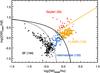 |
Fig. 17 Standard emission-line diagnostic diagram for CALIFA galaxies with SDSS spectra. Only spectra centered on the galaxy nucleus (<3′′) and with S/N > 3 in all emission lines are shown here. The demarcation lines by Kewley et al. (2001; black), Kauffmann et al. (2003b; black dotted), and Cid Fernandes et al. (2010; yellow) are used to characterize the objects into star forming (black), Seyferts (red), SF/AGN intermediates (blue), and LINER-like (orange) objects. The number of objects per class is indicated on the plot. |
8.2. X-ray luminosities
When the X-ray luminosity of a source exceeds log (L2−10 keV/ [ erg s-1 ] ) > 42 (e.g. Szokoly et al. 2004) in the soft or log (L15−195 keV/ [ erg s-1 ] ) > 42.2 in the hard band, it is most likely harbouring an AGN. A large fraction of soft X-ray photons are absorbed in obscured (type 2) AGN, so the ROSAT all-sky survey (Voges et al. 1999) does not efficiently identify the low-luminosity type 2 AGN that dominate the AGN population in CALIFA. Instead, we matched the CALIFA galaxies with the Swift BAT 70-month hard X-ray survey (Baumgartner et al. 2013) that contains 15 confirmed counterparts with log (L15−195 keV/ [erg s-1]) > 42.2 clearly indicative of AGN. This hard X-ray sample includes Mrk 79, which is a well-known type 1 AGN that is part of the CALIFA sample.
8.3. The incidence of radio AGN
A completely different signature of nuclear activity is the jets released from the AGN that can be identified by their enhanced radio emission. Ongoing star formation usually produces also some level of radio emission, but the number density of radio-AGN dominates over that of star forming galaxies above a radio continuum luminosity of L1.4 GHz > 1023 W Hz-1 (Best & Heckman 2012). The radio luminosity distribution of CALIFA galaxies detected by the NVSS survey is shown in Fig. 18. We identified 15 galaxies with L1.4 GHz > 1023 W Hz-1 in the CALIFA MS for which we carefully checked the radio morphology in the corresponding NVSS and FIRST images, when available. Removing the known ULIRG Arp 220, 11 of these show either clear jet-like structure or are hosted in bulge-dominated galaxies for which strong star formation is not expected.
For galaxies with L1.4 GHz < 1023 W Hz-1 it is difficult to identify the origin of the radio emission without additional indications. Here we used the criterion introduced by Best et al. (2005), incorporating the 4000 Å break strength (D4000N index). The 4000 Å break strength was taken from the analysis of the SDSS DR7 spectra which reduced the sample again to 582 objects. Because the 3′′ apertures of the SDSS fibres cover only the central part of the galaxy we excluded all radio sources with extended emission that follows that of the host galaxy. With the 4000 Å break strength as an age indicator of the stellar population we can identify 17 additional potential radio AGN. These are predominantly located in elliptical or lenticular galaxies that display no significant emission lines or LINER-type spectra. The only object in common between the three type 1 AGN samples here is NGC 4874, which is a cD galaxy detected in the radio and the X-rays.
This short accounting shows that based on the evidence available prior to the CALIFA spectroscopy, the AGN fraction in CALIFA galaxies appears to be around 6%. Even if this low fraction should be confirmed there will still be approximately 30 AGN host galaxies for which the CALIFA data will provide detailed insights.
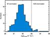 |
Fig. 18 Histogram of NVSS continuum radio luminosities at 1.4 GHz for all detected CALIFA objects. |
9. Summary
This paper is devoted to a detailed description of the CALIFA mother sample (MS). The main feature of the CALIFA sample is that it has been selected by diameter to fill the field of view of the IFU. The observed sample will be a randomly selected subset of the MS and will thus share all its properties, albeit with somewhat reduced statistical power. To fully characterize the sample, we have derived or collected a number of properties for its galaxies, in particular integrated optical magnitudes, stellar masses, and five different environmental measures, and we have identified AGN. Secondary data products derived in the context of this paper will be made available on the webpage of the CALIFA survey (http://www.caha.es/CALIFA/).
We conclude the following:
-
The MS is representative for the general galaxy population withthe following limits: −19.0 to −23.1 in r-band absolute magnitude, 1.7 to 11.5 kpc in half light radii, and 9.7 to 11.4 in log(stellar mass/M⊙).
-
Below Mr,p = −19, the MS contains mostly edge-on galaxies elevated into the sample by projection effects acting on their half-light major axes. Above Mr,p = −23.1 the CALIFA sample is limited by the total available volume in the sense that such luminous galaxies are very rare and thus are not represented in the volume available within our redshift limits.
-
The application of volume corrections allows the derivation of space densities and distribution functions of any measurable galaxy physical property from the CALIFA sample. We have derived the necessary corrections for the local underdensity of the Universe.
-
More than 97% of CALIFA galaxies are covered out to more than 2 × r50 at a typical spatial resolution of 1 kpc in the mean.
-
The sample covers all environments, from field galaxies to cluster environments, from isolated to interacting to merging galaxies.
-
The sample contains few easily identified, luminous AGN as these are rare in the local galaxy population. Nevertheless, the final observed sample will contain approximately 30 Seyfert galaxies.
Future IFS surveys should feel encouraged to consider diameter selection, as it provides an efficient use of the field of view and – as we have shown in this paper – leads to a controlled sample with benign properties. While future IFS surveys will probably be superior to CALIFA in sample size, we stress that CALIFA will occupy a unique place in parameter space for a long time to come in its combination of field of view, spatial resolution and S/N, which larger surveys will struggle to match due to limits imposed by spectrograph and detector sizes, i.e. by the number of resolution elements.
The exact meaning of all SDSSpipeline parameters is explained on the relevant DR7 webpage: http://cas.sdss.org/astrodr7/en/help/browser/browser.asp
SIMBAD is a database that experiences frequent updates, such that the only way we can reference the “release” is by date – January 15th 2010.
Note that this fraction drops to 50% when using the more accurate re from the growth curve analysis in Sect. 6.1, but the number given in the text above provides a natural comparison to other surveys.
Acknowledgments
This study makes uses of the data provided by the Calar Alto Legacy Integral Field Area (CALIFA) survey (http://califa.caha.es). CALIFA is the first legacy survey being performed at Calar Alto. The CALIFA collaboration would like to thank the IAA-CSIC and MPIA-MPG as major partners of the observatory, and CAHA itself, for the unique access to telescope time and support in manpower and infrastructures. The CALIFA collaboration thanks also the CAHA staff for the dedication to this project. We thank Mike Blanton for helpful discussions on the SDSS survey footprint and for providing the NYU low-z catalogue to the community. CJW acknowledges useful discussion with Nick Scott, Davor Krajnovic and Remco van den Bosch as well as support through the Marie Curie Career Integration Grant 303912. We thank the anonymous referee for a careful reading of the paper and several suggestions that improved its presentation. IM acknowledges the financial support from the Spanish grant AYA2010-15169 and from the Junta de Andalucia through TIC-114 and the Excellence Project P08-TIC-03531. R.G.D., E.P. and R.G.B. acknowledge support from the Spanish Ministerio de Economia y Competitividad, through projects AYA2010-15081. RAM is funded by the Spanish programme of International Campus of Excellence Moncloa (CEI). J.I.P. acknowledges financial support from the Spanish MINECO under grant AYA2010-21887-C04-01 and from Junta de Andalucía Excellence Project PEX2011-FQM7058. Support for L.G. is provided by the Ministry of Economy, Development, and Tourism’s Millennium Science Initiative through grant IC12009, awarded to The Millennium Institute of Astrophysics, MAS. L.G. acknowledges support by CONICYT through FONDECYT grant 3140566. AM.-I. acknowledges support from Agence Nationale de la Recherche through the STILISM project (ANR-12-BS05-0016-02). AM.-I. and S.B. acknowledge support from BMBF through the Erasmus-F project (grant number 05 A12BA1). JMA acknowledges support from the European Research Council Starting Grant (SEDmorph; P.I. V. Wild). A.G. acknowledges funding from the European Union Seventh Framework Programme (FP7/2007-2013) under grant agreement No. 267251. K.S. acknowledges financial support from the Natural Sciences and Engineering Research Council of Canada (NSERC). B.J. acknowledges support by the projects RVO67985815 and M100031201 of the Academy of Sciences of the Czech Republic. This research has made use of the NASA/IPAC Extragalactic Database (NED), which is operated by the Jet Propulsion Laboratory, California Institute of Technology, under contract with the National Aeronautics and Space Administration. This research has made use of the SIMBAD database, operated at CDS, Strasbourg, France. We acknowledge the usage of the HyperLeda database (http://leda.univ-lyon1.fr). Funding for the Sloan Digital Sky Survey (SDSS) has been provided by the Alfred P. Sloan Foundation, the Participating Institutions, the National Aeronautics and Space Administration, the National Science Foundation, the US Department of Energy, the Japanese Monbukagakusho, and the Max Planck Society. The SDSS Web site is http://www.sdss.org/. The SDSS is managed by the Astrophysical Research Consortium (ARC) for the Participating Institutions. The Participating Institutions are The University of Chicago, Fermilab, the Institute for Advanced Study, the Japan Participation Group, The Johns Hopkins University, Los Alamos National Laboratory, the Max-Planck-Institute for Astronomy (MPIA), the Max-Planck-Institute for Astrophysics (MPA), New Mexico State University, University of Pittsburgh, Princeton University, the United States Naval Observatory, and the University of Washington.
References
- Abazajian, K. N., Adelman-McCarthy, J. K., Agüeros, M. A., et al. 2009, ApJS, 182, 543 [NASA ADS] [CrossRef] [Google Scholar]
- Aguerri, J. A. L., Sánchez-Janssen, R., & Muñoz-Tuñón, C. 2007, A&A, 471, 17 [NASA ADS] [CrossRef] [EDP Sciences] [Google Scholar]
- Aguerri, J. A. L., Méndez-Abreu, J., & Corsini, E. M. 2009, A&A, 495, 491 [NASA ADS] [CrossRef] [EDP Sciences] [Google Scholar]
- Baldry, I. K., Balogh, M. L., Bower, R. G., et al. 2006, MNRAS, 373, 469 [NASA ADS] [CrossRef] [Google Scholar]
- Baldwin, J. A., Phillips, M. M., & Terlevich, R. 1981, PASP, 93, 5 [NASA ADS] [CrossRef] [EDP Sciences] [Google Scholar]
- Balogh, M. L., Baldry, I. K., Nichol, R., et al. 2004a, ApJ, 615, L101 [NASA ADS] [CrossRef] [Google Scholar]
- Balogh, M., Eke, V., Miller, C., et al. 2004b, MNRAS, 348, 1355 [Google Scholar]
- Baumgartner, W. H., Tueller, J., Markwardt, C. B., et al. 2013, ApJ, 207, 19 [Google Scholar]
- Berlind, A. A., Frieman, J., Weinberg, D. H., et al. 2006, ApJS, 167, 1 [NASA ADS] [CrossRef] [Google Scholar]
- Bershady, M. A., Verheijen, M. A. W., Swaters, R. A., et al. 2010, ApJ, 716, 198 [NASA ADS] [CrossRef] [Google Scholar]
- Bertin, E., & Arnouts, S. 1996, A&AS, 117, 393 [NASA ADS] [CrossRef] [EDP Sciences] [Google Scholar]
- Best, P. N., & Heckman, T. M. 2012, MNRAS, 421, 1569 [NASA ADS] [CrossRef] [Google Scholar]
- Best, P. N., Kauffmann, G., Heckman, T. M., et al. 2005, MNRAS, 362, 25 [NASA ADS] [CrossRef] [Google Scholar]
- Binggeli, B., Sandage, A., & Tammann, G. A. 1985, AJ, 90, 1681 [NASA ADS] [CrossRef] [Google Scholar]
- Blanton, M. R., & Roweis, S. 2007, AJ, 133, 734 [NASA ADS] [CrossRef] [Google Scholar]
- Blanton, M. R., Dalcanton, J., Eisenstein, D., et al. 2001, AJ, 121, 2358 [NASA ADS] [CrossRef] [Google Scholar]
- Blanton, M. R., Hogg, D. W., Bahcall, N. A., et al. 2003, ApJ, 592, 819 [NASA ADS] [CrossRef] [Google Scholar]
- Blanton, M. R., Schlegel, D. J., Strauss, M. A., et al. 2005a, AJ, 129, 2562 [NASA ADS] [CrossRef] [Google Scholar]
- Blanton, M. R., Lupton, R. H., Schlegel, D. J., et al. 2005b, ApJ, 631, 208 [NASA ADS] [CrossRef] [Google Scholar]
- Boselli, A., & Gavazzi, G. 1994, A&A, 283, 12 [NASA ADS] [Google Scholar]
- Bruzual, G., & Charlot, S. 2003, MNRAS, 344, 1000 [NASA ADS] [CrossRef] [Google Scholar]
- Cappellari, M., Emsellem, E., Krajnović, D., et al. 2011, MNRAS, 413, 813 [NASA ADS] [CrossRef] [Google Scholar]
- Chabrier, G. 2003, PASP, 115, 763 [NASA ADS] [CrossRef] [Google Scholar]
- Cid Fernandes, R., Stasińska, G., Schlickmann, M. S., et al. 2010, MNRAS, 403, 1036 [NASA ADS] [CrossRef] [Google Scholar]
- Corwin, Jr., H. G.,Buta, R. J., & de Vaucouleurs, G. 1994, AJ, 108, 2128 [NASA ADS] [CrossRef] [Google Scholar]
- Crook, A. C., Huchra, J. P., Martimbeau, N., et al. 2007, ApJ, 655, 790 [NASA ADS] [CrossRef] [Google Scholar]
- Davies, J. I. 1990, MNRAS, 244, 8 [NASA ADS] [Google Scholar]
- Davis, M., Faber, S. M., Newman, J., et al. 2003, in SPIE Conf. Ser. 4834, ed. P. Guhathakurta, 161 [Google Scholar]
- de Jong, R. S., & van der Kruit, P. C. 1994, A&AS, 106, 451 [NASA ADS] [Google Scholar]
- De Lucia, G., Weinmann, S., Poggianti, B. M., Aragón-Salamanca, A., & Zaritsky, D. 2012, MNRAS, 423, 1277 [NASA ADS] [CrossRef] [Google Scholar]
- de Vaucouleurs, G., de Vaucouleurs, A., Corwin, Jr., H. G., et al. 1991, Third Reference Catalogue of Bright Galaxies. Volume I: Explanations and references. Volume II: Data for galaxies between 0h and 12h. Volume III: Data for galaxies between 12h and 24h, (New York: Springer) [Google Scholar]
- de Zeeuw, P. T., Bureau, M., Emsellem, E., et al. 2002, MNRAS, 329, 513 [NASA ADS] [CrossRef] [Google Scholar]
- Disney, M., Davies, J., & Phillipps, S. 1989, MNRAS, 239, 939 [NASA ADS] [CrossRef] [Google Scholar]
- Eisenstein, D. J., Annis, J., Gunn, J. E., et al. 2001, AJ, 122, 2267 [NASA ADS] [CrossRef] [Google Scholar]
- Finn, R. A., Zaritsky, D., McCarthy, Jr., D. W., et al. 2005, ApJ, 630, 206 [NASA ADS] [CrossRef] [Google Scholar]
- Ganda, K., Falcón-Barroso, J., Peletier, R. F., et al. 2006, MNRAS, 367, 46 [NASA ADS] [CrossRef] [Google Scholar]
- Garcia, A. M. 1993, A&AS, 100, 47 [NASA ADS] [Google Scholar]
- Gavazzi, G., Boselli, A., Scodeggio, M., Pierini, D., & Belsole, E. 1999, MNRAS, 304, 595 [NASA ADS] [CrossRef] [Google Scholar]
- Gavazzi, G., Boselli, A., Donati, A., Franzetti, P., & Scodeggio, M. 2003, A&A, 400, 451 [NASA ADS] [CrossRef] [EDP Sciences] [Google Scholar]
- Gavazzi, G., Fumagalli, M., Cucciati, O., & Boselli, A. 2010, A&A, 517, A73 [NASA ADS] [CrossRef] [EDP Sciences] [Google Scholar]
- Gil de Paz, A., Boissier, S., Madore, B. F., et al. 2007, ApJS, 173, 185 [NASA ADS] [CrossRef] [Google Scholar]
- Hernández-Fernández, J. D., Iglesias-Páramo, J., & Vílchez, J. M. 2012, ApJS, 199, 22 [NASA ADS] [CrossRef] [Google Scholar]
- Hickson, P. 1982, ApJ, 255, 382 [NASA ADS] [CrossRef] [Google Scholar]
- Husemann, B., Jahnke, K., Sánchez, S. F., et al. 2013, A&A, 549, A87 [NASA ADS] [CrossRef] [EDP Sciences] [Google Scholar]
- Jarrett, T.-H., Chester, T., Cutri, R., et al. 2000, AJ, 120, 298 [NASA ADS] [CrossRef] [Google Scholar]
- Jordi, K., Grebel, E. K., & Ammon, K. 2006, A&A, 460, 339 [NASA ADS] [CrossRef] [EDP Sciences] [Google Scholar]
- Karachentsev, I. D. 1972, Soobshcheniya Spetsial’noj Astrofizicheskoj Observatorii, 7, 1 [Google Scholar]
- Karachentseva, V. E., Karachentsev, I. D., & Lebedev, V. S. 1987, Bulletin d’Information du Centre de Données Stellaires, 32, 81 [NASA ADS] [Google Scholar]
- Kauffmann, G., Heckman, T. M., Tremonti, C., et al. 2003b, MNRAS, 346, 1055 [Google Scholar]
- Kelz, A., Verheijen, M. A. W., Roth, M. M., et al. 2006, PASP, 118, 129 [NASA ADS] [CrossRef] [Google Scholar]
- Kewley, L. J., Dopita, M. A., Sutherland, R. S., Heisler, C. A., & Trevena, J. 2001, ApJ, 556, 121 [Google Scholar]
- Kniazev, A. Y., Grebel, E. K., Pustilnik, S. A., et al. 2004, AJ, 127, 704 [NASA ADS] [CrossRef] [Google Scholar]
- Lackner, C. N., & Gunn, J. E. 2012, MNRAS, 421, 2277 [NASA ADS] [CrossRef] [Google Scholar]
- Le Fèvre, O., Vettolani, G., Garilli, B., et al. 2005, A&A, 439, 845 [NASA ADS] [CrossRef] [EDP Sciences] [Google Scholar]
- Mahdavi, A., & Geller, M. J. 2001, ApJ, 554, L129 [NASA ADS] [CrossRef] [Google Scholar]
- Mahdavi, A., & Geller, M. J. 2004, ApJ, 607, 202 [NASA ADS] [CrossRef] [Google Scholar]
- Mahtessian, A. P., & Movsessian, V. G. 2010, ApJ, 53, 70 [Google Scholar]
- Maller, A. H., Berlind, A. A., Blanton, M. R., & Hogg, D. W. 2009, ApJ, 691, 394 [NASA ADS] [CrossRef] [Google Scholar]
- Miller, C. J., Nichol, R. C., Reichart, D., et al. 2005, AJ, 130, 968 [Google Scholar]
- Mould, J. R., Huchra, J. P., Freedman, W. L., et al. 2000, ApJ, 529, 786 [NASA ADS] [CrossRef] [Google Scholar]
- Moustakas, J., Coil, A. L., Aird, J., et al. 2013, ApJ, 767, 50 [NASA ADS] [CrossRef] [Google Scholar]
- Nilson, P. 1973, Uppsala general catalogue of galaxies [Google Scholar]
- Öpik, E. 1923, The Observatory, 46, 51 [NASA ADS] [Google Scholar]
- Padilla, N. D., & Strauss, M. A. 2008, MNRAS, 388, 1321 [NASA ADS] [Google Scholar]
- Paturel, G., Petit, C., Prugniel, P., et al. 2003, A&A, 412, 45 [NASA ADS] [CrossRef] [EDP Sciences] [Google Scholar]
- Poggianti, B. M., von der Linden, A., De Lucia, G., et al. 2006, ApJ, 642, 188 [NASA ADS] [CrossRef] [Google Scholar]
- Popesso, P., Biviano, A., Böhringer, H., & Romaniello, M. 2007, A&A, 461, 397 [NASA ADS] [CrossRef] [EDP Sciences] [Google Scholar]
- Rines, K., Geller, M. J., Kurtz, M. J., & Diaferio, A. 2003, AJ, 126, 2152 [NASA ADS] [CrossRef] [Google Scholar]
- Roth, M. M., Kelz, A., Fechner, T., et al. 2005, PASP, 117, 620 [NASA ADS] [CrossRef] [Google Scholar]
- Sánchez, S. F., Kennicutt, R. C., Gil de Paz, A., et al. 2012a, A&A, 538, A8 [NASA ADS] [CrossRef] [EDP Sciences] [Google Scholar]
- Sánchez, S. F., Rosales-Ortega, F. F., Marino, R. A., et al. 2012b, A&A, 546, A2 [NASA ADS] [CrossRef] [EDP Sciences] [Google Scholar]
- Schmidt, M. 1968, ApJ, 151, 393 [NASA ADS] [CrossRef] [Google Scholar]
- Shen, S., Kauffmann, G., von der Linden, A., White, S. D. M., & Best, P. N. 2008, MNRAS, 389, 1074 [NASA ADS] [CrossRef] [Google Scholar]
- Strateva, I., Ivezić, Ž., Knapp, G. R., et al. 2001, AJ, 122, 1861 [Google Scholar]
- Strauss, M. A., Weinberg, D. H., Lupton, R. H., et al. 2002, AJ, 124, 1810 [NASA ADS] [CrossRef] [Google Scholar]
- Szokoly, G. P., Bergeron, J., Hasinger, G., et al. 2004, ApJS, 155, 271 [NASA ADS] [CrossRef] [Google Scholar]
- Tago, E., Saar, E., Tempel, E., et al. 2010, A&A, 514, A102 [NASA ADS] [CrossRef] [EDP Sciences] [Google Scholar]
- Tempel, E., Tago, E., & Liivamägi, L. J. 2012, A&A, 540, A106 [NASA ADS] [CrossRef] [EDP Sciences] [Google Scholar]
- Tremonti, C. A., Heckman, T. M., Kauffmann, G., et al. 2004, ApJ, 613, 898 [NASA ADS] [CrossRef] [Google Scholar]
- Unterborn, C. T., & Ryden, B. S. 2008, ApJ, 687, 976 [NASA ADS] [CrossRef] [Google Scholar]
- Varela, J., Moles, M., Márquez, I., et al. 2004, A&A, 420, 873 [NASA ADS] [CrossRef] [EDP Sciences] [Google Scholar]
- Verdes-Montenegro, L., Sulentic, J., Lisenfeld, U., et al. 2005, A&A, 436, 443 [NASA ADS] [CrossRef] [EDP Sciences] [Google Scholar]
- Verheijen, M., Bershady, M., Andersen, D., et al. 2004, Astron. Nachr., 325, 151 [NASA ADS] [CrossRef] [Google Scholar]
- Voges, W., Aschenbach, B., Boller, T., et al. 1999, A&A, 349, 389 [NASA ADS] [Google Scholar]
- Walcher, C. J., Lamareille, F., Vergani, D., et al. 2008, A&A, 491, 713 [NASA ADS] [CrossRef] [EDP Sciences] [Google Scholar]
- Walcher, J., Groves, B., Budavári, T., & Dale, D. 2011, Ap&SS, 331, 1 [NASA ADS] [CrossRef] [Google Scholar]
- Wang, L., Yang, X., Luo, W., et al. 2011, ApJ, submitted [arXiv:1110.1987] [Google Scholar]
- White, D. A., Jones, C., & Forman, W. 1997, MNRAS, 292, 419 [NASA ADS] [CrossRef] [Google Scholar]
- Willett, K. W., Lintott, C. J., Bamford, S. P., et al. 2013, MNRAS, 435, 2835 [NASA ADS] [CrossRef] [Google Scholar]
- Yang, X., Mo, H. J., van den Bosch, F. C., et al. 2007, ApJ, 671, 153 [NASA ADS] [CrossRef] [Google Scholar]
All Tables
All Figures
|
Fig. 1 Left panel: the footprint on the sky of our search in the DR7 CAS (light blue) and the distribution of the 939 galaxies constituting the CALIFA mother sample (red circles). Right panels: redshifts vs. absolute magnitudes Mr,GC (top) and r-band linear isophotal sizes (bottom) for the galaxies in the sample. The dotted lines in the lower panel are the selection limits. |
| In the text | |
|
Fig. 2 Left: histogram of radial coverages of the CALIFA galaxies, i.e. the ratio between the radius of the Field of View of PPak and petroR50r. This figure does not give the actual spectroscopic coverage, which may be smaller due to S/N issues. Right: histogram of spatial scales with which the CALIFA galaxies are observed. A fibre diameter is 2.7′′, whereas the typical fibre-to-fibre distance is 3′′. The final spatial resolution of CALIFA will depend on future optimizations of the cubing code, but will be approximately 3′′. |
| In the text | |
|
Fig. 3 Selection limits of CALIFA: absolute magnitudes Mr,p are plotted against linear isophotal sizes of galaxies in the CALIFA MS (black points), compared to the same for galaxies in SDSS (orange). The two vertical dashed lines delineate the range of galaxies accessible to CALIFA; all galaxies within this range would be selected by CALIFA if located at a suitable redshift. The horizontal lines represent the limits inside which for a certain luminosity bin the fraction of SDSS galaxies within the CALIFA “accessible range” is above 95%. |
| In the text | |
|
Fig. 4 Fraction of SDSS galaxies within the CALIFA accessible range of Diso, as a function of absolute magnitude. Error bars are Poissonian. The two vertical lines bracket the range where the fraction is >95%. |
| In the text | |
|
Fig. 5 As Fig. 4, but showing the fraction as a function of half-light radius (i.e. SDSS pipeline r50). The two vertical lines again bracket the range where the fraction is >95%. |
| In the text | |
|
Fig. 6 Available survey volume for all galaxies in the CALIFA MS, as a function of linear isophotal size as derived from the observed redshift. |
| In the text | |
|
Fig. 7 Top: observed (black) and predicted (blue) number of SDSS galaxies with magnitudes r < 17.7 per Δz = 0.002 redshift bin. Bottom: ratio of these two numbers, as a function of redshift. |
| In the text | |
|
Fig. 8 The red points show the r band luminosity function of galaxies estimated from the CALIFA MS, using absolute magnitudes from the SDSS Mr,p and with error bars representing Poissonian uncertainties only. The orange squares are for the same sample, but without the corrections for variations in cosmic density. The blue solid line shows the Schechter fit to the LF of Blanton et al. (2003), adjusted to our cosmology and redshift range. The vertical dashed lines indicate the completeness limits derived in Sect. 3.2. The faintest magnitude at which the luminosity function itself is marginally consistent with that of Blanton et al. would imply that the limit of completeness for the CALIFA sample is at roughly Mr,p < −18.6. |
| In the text | |
|
Fig. 9 Distribution function of linear isophotal sizes Diso of galaxies estimated from the CALIFA sample, compared to the same distribution constructed by us from the SDSS low-z subsample. Symbols and line types as in Fig. 8. |
| In the text | |
|
Fig. 10 Histogram of axis ratios (2nd order moments of the r band light distribution) for the CALIFA MS. Overplotted in blue is the histogram for disc-dominated systems with Mr,p < −18.6 and concentration indices c < 2.6, and in red for comparison the axis ratio distribution (rescaled to the same number of objects) for the disc-dominated galaxies in the SDSS sample of Maller et al. (2009). |
| In the text | |
|
Fig. 11 Histogram of isophotal axis ratios (at 25 mag/arcsec2 level) for the CALIFA MS. Overplotted with a dotted line is the histogram for the 55 low-luminosity systems with Mr,p > −18.6, which are almost all highly inclined disc systems. |
| In the text | |
|
Fig. 12 Relation between absolute magnitudes (Mr,p, uncorrected for internal extinction) and linear isophotal sizes of the CALIFA MS, colour–coded according to isophotal axis ratios. |
| In the text | |
|
Fig. 13 Left panel: comparison of apparent magnitudes obtained from growth curve measurements with those from the SDSS pipeline (petroMagr). Right panel: comparison of apparent g magnitudes obtained from growth curve measurements with estimates of the same derived from the RC3. Both panels show typical error bars in the upper left corner. |
| In the text | |
|
Fig. 14 Left panel: distribution of stellar masses in the CALIFA sample from a fit to the optical spectral energy distribution. Right panel: mass function of the CALIFA mother sample compared with the mass function from Moustakas et al. (2013). The two vertical lines indicate the representativity limits derived using the same method as in Sect. 3.2 from the low-z SDSS comparison sample: 9.65 < log (M⋆/M⊙) < 11.44. |
| In the text | |
|
Fig. 15 Distribution of morphological types in the CALIFA sample from our own classification. Independent histograms are drawn by bar classification as non-barred (meanbar = A, full line, dark blue), strong bar (meanbar = B, dashed, blue) and weak bar (meanbar = AB, dotted, red). |
| In the text | |
|
Fig. 16 Left panel: comparison between a pair of related environment measures. The mass of the host halo from the Wang et al. (2011) catalogue vs. the velocity dispersion of the closest known structure compiled in this work. Right panel: stellar mass distribution of members in known structures. The largest known structures have been identified. Galaxies have been colour coded by their morphological classification. |
| In the text | |
|
Fig. 17 Standard emission-line diagnostic diagram for CALIFA galaxies with SDSS spectra. Only spectra centered on the galaxy nucleus (<3′′) and with S/N > 3 in all emission lines are shown here. The demarcation lines by Kewley et al. (2001; black), Kauffmann et al. (2003b; black dotted), and Cid Fernandes et al. (2010; yellow) are used to characterize the objects into star forming (black), Seyferts (red), SF/AGN intermediates (blue), and LINER-like (orange) objects. The number of objects per class is indicated on the plot. |
| In the text | |
|
Fig. 18 Histogram of NVSS continuum radio luminosities at 1.4 GHz for all detected CALIFA objects. |
| In the text | |
Current usage metrics show cumulative count of Article Views (full-text article views including HTML views, PDF and ePub downloads, according to the available data) and Abstracts Views on Vision4Press platform.
Data correspond to usage on the plateform after 2015. The current usage metrics is available 48-96 hours after online publication and is updated daily on week days.
Initial download of the metrics may take a while.