| Issue |
A&A
Volume 568, August 2014
|
|
|---|---|---|
| Article Number | A36 | |
| Number of page(s) | 9 | |
| Section | Extragalactic astronomy | |
| DOI | https://doi.org/10.1051/0004-6361/201322736 | |
| Published online | 11 August 2014 | |
Modelling photometric reverberation data: a disk-like broad-line region and a potentially larger black hole mass for 3C 120
1 Astronomisches Institut, Ruhr-Universität Bochum, Universitätsstraße 150, 44801 Bochum, Germany
e-mail: This email address is being protected from spambots. You need JavaScript enabled to view it.
2 Instituto de Astronomía, Universidad Católica del Norte, Avenida Angamos 0610, Casilla 1280 Antofagasta, Chile
3 Department of Physics, University of Oxford, Keble Road, Oxford OX1 3RH, UK
4 Departamento de Física, Universidad Católica del Norte, Avenida Angamos 0610, Casilla 1280 Antofagasta, Chile
5 Institut für Astrophysik, Universität Göttingen, Friedrich-Hund-Platz 1, 37077 Göttingen, Germany
Received: 23 September 2013
Accepted: 23 June 2014
Abstract
We consider photometric reverberation mapping, where the nuclear continuum variations are monitored via a broad-band filter and the echo of emission line clouds of the broad-line region (BLR) is measured with a suitable narrow-band (NB) filter. We investigate how an incomplete emission-line coverage by the NB filter influences the determination of the BLR size. This includes two basic cases: 1) a symmetric cut of the blue and red part of the line wings; and 2) the filter positioned asymmetrically to the line centre so that essentially a complete half of the emission line is contained in the NB filter. Under the assumption that the BLR is dominated by circular Keplerian orbits, we find that symmetric cutting of line wings may lead to overestimating the BLR size by less than 5%. The case of asymmetric half-line coverage, similar as for our data of the Seyfert 1 galaxy 3C 120, yields a BLR size with a bias of less than 1%. Our results suggest that any BLR size bias due to a narrow-band line cut in photometric reverberation mapping is small and in most cases negligible. We used well-sampled photometric reverberation mapping light curves with sharp variation features in both the continuum and the Hβ light curves to determine the geometry type of the Hβ BLR for 3C 120. Modelling of the light curve, under the assumption that the BLR is essentially virialised, argues against a spherical geometry and favours a nearly face-on disk-like geometry with an inclination i = 10° ± 4° and an extension from 22 to 28 light days. The low inclination may lead to a larger black hole mass MBH than that derived when using the average geometry scaling factor f = 5.5. We discuss deviations of Seyfert 1 galaxies from the MBH–σ∗ relation.
Key words: galaxies: Seyfert / quasars: emission lines / galaxies: distances and redshifts / galaxies: individual: 3C 120 / galaxies: active
© ESO, 2014
1. Introduction
The broad-line region (BLR) of active galactic nuclei (AGNs) has been studied for over 40 years. In our current understanding of the structure of the central engine of AGNs, the observed broad emission lines are photo-ionised by the central ionising source located close to the super-massive black hole (SMBH), which emits high-energy photons as a consequence of matter falling into the SMBH. The broad emission lines respond to the strong and variable optical/UV continuum at remarkably short time-scales, and are thus at small distances (about 1 to 250 light days) from the accretion disk (AD) (e.g., Kaspi et al. 2000; Bentz et al. 2009). For a virialised BLR with known geometry the mass MBH of the SMBH can be determined.
Reverberation mapping (RM, Lyutyi & Cherepashchuk 1972; Cherepashchuk & Lyutyi 1973; Blandford & McKee 1982; Gaskell & Sparke 1986; Peterson 1993) allows us, independent of spatial resolution, to infer the size and morphology of the BLR. Spectroscopic monitoring measures the time delay (τBLR = RBLR/c) between changes in the optical-ultraviolet continuum produced in the compact AD and the emission line from the BLR gas clouds farther out. If the BLR clouds are essentially in virialised motion around the black hole (e.g., Peterson & Wandel 1999; Krolik 2001; Onken & Peterson 2002; Kollatschny 2003b), combining the velocity dispersion of the BLR gas (σV) with the BLR size (RBLR = c·τBLR) allows us to estimate the virial BH mass using  , where G is the gravitational constant, and the factor f depends on the geometry and kinematics of the BLR (Peterson et al. 2004, and references therein). The commonly used average factor f of a small sample of AGN (Onken et al. 2004) may lead to a large scatter in MBH and in relationships involving MBH (Peterson et al. 2004). To improve these relationships one needs to determine f more precisely for each AGN.
Geometric models for spherical inflow, outflow, and disk BLR structures have been constructed by interpreting the RM transfer function as a two-dimensional map, the well-known “echo image” of the BLR (Welsh & Horne 1991; Horne 2003). Although there is no clear consensus about the geometry of the BLR, past studies have shown evidence in favour of a disk-like configuration (e.g., Wills & Browne 1986; Murray & Chiang 1997; Bottorff et al. 1997; Elvis 2000; Konigl & Kartje 1994; Kollatschny 2003a,b; Kollatschny & Zetzl 2011, 2013). Kollatschny & Zetzl (2011, 2013) analysed the shape of the rms line profiles of a homogenous AGN subsample of Peterson et al. (2004) and found evidence for the superposition of rotational disk-like components and turbulence.
The velocity-resolved (two-dimensional) RM of Mrk 110 (Kollatschny 2003a) has best been explained with a dominating disk-like BLR component at inclination ~20° (i.e. close to face-on), consistent with the detected gravitational redshift (Kollatschny 2003b). By using Bayesian probability theory and Monte Carlo algorithms, Pancoast et al. (2011) presented a general method for geometric and dynamical modelling of the BLR. Using this method, Brewer et al. (2011) and Pancoast et al. (2012) modelled the geometry and estimated the BH mass for the Seyfert 1 galaxies Arp 151 and Mrk 50. In both studies evidence for a disk-like BLR geometry was found. The broad-line radio galaxy 3C 120 has been observed with velocity-resolved RM at two different epochs (Grier et al. 2012 and Kollatschny et al. 2014). Below we discuss details of this when we compare their results with our data (Sect. 2).
In general terms, any modelling to infer the BLR geometry requires high time-resolution observations and pronounced well-defined variability features in the light curves. Spectrophotometric light curves are to date the main source of observational data for RM. So far, velocity-resolved RM has been the only method used to study the geometry of the BLR with high precision. Because the method is resource expensive, it is desirable to explore whether the basic features of the BLR geometry can be inferred directly from photometric monitoring data.
Recently, photometric reverberation mapping (PRM) has been revisited as an efficient method for determining the BLR size by combining narrow- and broad-band filters (Haas et al. 2011; Pozo Nuñez et al. 2012, 2013) or by using only broad-band filters (Chelouche & Daniel 2012; Edri et al. 2012; Chelouche et al. 2012; Chelouche 2013; Chelouche & Zucker 2013). PRM may become an extremely powerful tool with unprecedented efficiency – in particular with respect to upcoming large surveys like the LSST. Before the PRM is widely used, however, the accuracy and possible biases have to be checked and established. Several such studies are under way.
By using well-sampled light curves obtained for 3C 120, we demonstrated that the Hβ BLR size R(Hβ) obtained by PRM is consistent with that from spectroscopic RM (Pozo Nuñez et al. 2012, hereafter called Paper I). Similarly, with PRM we measured R(Hα) of the narrow-line Seyfert 1 galaxy ESO399-IG20 (Pozo Nuñez et al. 2013, hereafter called Paper II). It places ESO399-IG20 extremely well within the R–L relationship (refined by Bentz et al. 2009), which supports the correctness of the BLR size as derived from PRM. The strong Hα line contribution to the r band allows us to derive R(Hα) even with the pure broad-band PRM techniques proposed by Chelouche & Daniel (2012). Furthermore, our PRM light curves of ESO399-IG20 show sharp variation features in both the triggering continuum and the emission line echo, enabling us – by means of simple BLR models – to find evidence in favour of a nearly face-on thin disk-like BLR geometry.
In Papers I and II we monitored the nuclear continuum variations via a broad-band (BB) filter, and the echo of emission line clouds of the BLR was measured with a suitable narrow-band (NB) filter. However, sometimes the NB filter is too narrow and thus cuts parts of the emission line (band width ~50 Å corresponding to a velocity coverage of ~3000 km s-1). The line wings correspond to BLR clouds with the fastest line of sight velocities. Assuming Keplerian motion, these clouds populate the innermost zones of the BLR. Thus, for photometric RM, one may expect that cutting the line wings may result in an overestimate of the BLR size. Another configuration is that the line is not centred on the NB filter. Another difficulty, related to incomplete line coverage due to the NB is to probe which conclusions about the BLR geometry can be drawn from such PRM data with truncated velocity information.
This paper deals with three topics: in Sect. 3 we investigate how an incomplete emission line coverage by the NB filter influences the BLR size determination. Specifically, we examine the bias of the BLR size 1) for a symmetric cut of the blue and red part of the line wings (Sect. 3.1); and 2) if the filter is positioned asymmetrically to the line centre so that essentially a complete half of the emission line is contained in the NB filter (Sect. 3.2). In Sect. 4, invoking reasonable assumptions from velocity resolved RM of 3C 120, we apply simple BLR models to the well-sampled PRM data of 3C 120. In this case, the sharp variation features in the PRM data enable us to constrain the BLR geometry of 3C 120. Since a nearly face-on disk-like BLR may lead to a larger black hole mass, we discuss the implications for the MBH–σ∗ relation in Sect. 5.
2. Data and model considerations
The source 3C 120 has been monitored spectroscopically – assisted by BB photometry – in 2008/2009 by Kollatschny et al. (2014, K+2014) and in 2010/2011 similarly by Grier et al. (2012, 2013, G+2013). The data by G+2013 are very well sampled, but catch only rather smooth variations in the light curves. The data by K+2014 show strong variations, but are not optimally sampled (median 6−8 days). Both G+2013 and K+2014 performed a velocity-resolved RM analysis, albeit with different techniques, and obtained mostly consistent but slightly different results. Both analyses found evidence for a disk-like BLR component, but G+2013 interpreted the red wing in the Hβ and Hγ lines as signature for inflowing gas, while K+2014 interpreted the red Balmer wings as optical-depth effects of a disk-wind (as proposed by Murray & Chiang 1997). Moreover, from the He lines, K+2014 found evidence for outflows, that appear to be more consistent with the expectations for this powerful broad-line radio galaxy having a superluminal jet pointing closely towards us (see Sect. 4.3).
The photometric RM data of 3C 120 that are examined here were observed in 2009/2010 (Paper I), between the two spectroscopic RM campaigns, when 3C 120 was in a lower luminosity state. In brief, we observed light curves in the B band, the [OIII] 5007 Å NB to catch the z = 0.033 redshifted Hβ line, and the V band to subtract host and continuum contribution from the Hβ light curve. Our well-sampled PRM light curves (median two days) show strong abrupt variations in both continuum and Hβ, but the velocity information is missing and the velocity range is truncated.
Before we describe the model in detail, we stress two general consideration.
Firstly, if the BLR has a spherical geometry, the front and back sides of the sphere will broaden the transfer function and thus will smear out the echo, which then looses its sharp features. The same holds for a disk-like BLR with high inclination i> 40° (i.e. intermediate to edge-on view). Because this smearing-out contradicts what is observed in our echo light curves of 3C 120, any spherical BLR or highly inclined BLR disk appears to be unlikely. This conclusion is independent of the kinematical model. In more general terms, the direct visual inspection of the light curves suggests that the sharp Hβ echoes, which perfectly follow the sharp continuum variations, exclude any BLR geometry, that is extended along the line of sight.
Secondly, if the kinematic model of the BLR (Kepler movement of gas clouds or outflow) is known, for instance from velocity-delay maps, and if the BLR is quasi-static during the observing campaign, the echo light curve solely depends on the location of the echoing gas clouds. This is why PRM data are able to provide constraints on the geometry.
We modelled the photometric RM data of 3C 120 in essentially the same way as we did for ESO399-IG20 in Paper II. The models are below characterised briefly.
Following Welsh & Horne (1991), we considered simple models. We assumed circular Keplerian orbits, thin disks, and/or spherical BLR geometry, with inner and outer radii (Rmin, Rmax). Consistent with the optimally emitting cloud model (Baldwin et al. 1995), we found and assumed modest ratios Rmax/Rmin< 2, and therefore used throughout a constant gas density independent of the cloud distance from the very centre, and a constant radiation efficiency ϵ.
We varied the thin-disk inclination i, and finally also used modestly thick inclined disks with covering half angles α. Our simple models do not account for in-/outflow, turbulence, projection effects, or for optical-depth effects in the disk-wind model of Murray & Chiang (1997).
3. Effect of cutting the line wings on the measured mean lags
Photometric reverberation mapping uses a NB filter to observe the emission line and a BB filter to observe the continuum. Here we examine the possible bias in lag determination caused by NB filter line-wing cutting. Line wings correspond to BLR clouds with the fastest line-of-sight velocities. The objective is to quantify the bias with simple models and to check photometric lag estimations. We restricted our investigation to thin disk-like BLR geometries, considering them as worst cases, because disks have a higher proportion of line wings (fast BLR clouds) than spherical BLRs, hence disks are more affected by line-cutting.
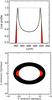 |
Fig. 1 Symmetric case of a thin disk-like BLR geometry (i = 45°, Rmin = 20 light days, Rmax = 30 light days, vmax = 3700 km s-1). Top: a rectangular filter (dotted line) is symmetrically centred on the spectral line (thick solid line); the parts of the line that are cut off by the filter are shaded in red. Bottom: BLR areas inside (black) and outside (red) of the filter. If a disk-like BLR-model with Keplerian orbits is assumed, the red shaded areas with the highest apparent velocity are cut off by the filter. |
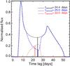 |
Fig. 2 Response of the BLR to a single light-pulse. The BLR is modelled as a thin circular Keplerian-disk. The dotted curves show the time-delay function of the entire BLR (black), the BLR part outside of the NB (red dotted line), and the BLR part inside of the NB (blue dashed line). The response of the entire emission line (black) can be separated into a part contained by the NB and a part outside the NB. The solid vertical lines mark the centroids of the filter answers (i.e. the mean time lag). The difference between the blue and the black centroid is the response (echo) bias. The value of the measured echo (blue) is higher than that of the real one (black). Thus, cutting line wings will (marginally) increase the mean time lag. |
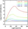 |
Fig. 3 Dependence of the time-lag over-estimate for a thin-disk BLR at inclination 45°. For each value of rmax/rmin, the curve shows the lag over-estimate as a function of line cut, here expressed as light lost. |
3.1. Symmetric case for a rectangular band-pass
We start with an inclined disk-like BLR and assumed a rectangular bandpass for the filter centred on the emission line, as illustrated in Fig. 1. At first glance, one expects that the average echo of these innermost clouds (with a velocity outside the band pass) arrives earlier than the mean echo of the complete disk.
The echo of an isotropic light-pulse from the (point-like) central accretion disk was calculated as shown in Fig. 2. The first echo peak lags the continuum pulse by about eight days. It originates from the front side of the ring, which is tilted towards the observer. The latest echo from the back side arrives about 40−50 days later than the continuum pulse. To compare this with the observations, we measured the mean lag by the centroid of the time-delay function, which corresponds to the centroid of the cross-correlation of two light curves. The mean true lag of the entire BLR is 24.4 days. The BLR part missed by the NB filter is that with the highest line-of-sight velocity, as shown in Fig. 2. The echo of this region has a mean lag of 22 days. But for the BLR covered by the NB, the measured echo has a mean lag of 25 days. This is only 2−3% more than the true mean BLR size. The reason for this remarkably small deviation between measured and true BLR size is that the loss occurs close to the centroid of the response function, while the outer parts remain unaffected (Fig. 2).
We computed the effect of line cutting for a range of parameters: inclination i, rmin and rmax, and MBH, i.e. vmax at rmin. vmax is the highest velocity seen at the given inclination i; in reality  /sin(i). The most important parameter – apart from the geometry type – is the ratio of rmin and rmax of a BLR, virialised with gas clouds on circular Keplerian orbits, and the percentage of light that is cut by the NB filter. The resulting over-estimations of the time lag are shown in Fig. 3. For typical cases rmax/rmin< 2; if the NB cuts off less than 10% (20%) of the line flux, the lag over-estimate is lower than 2% (~4%).
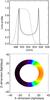 |
Fig. 4 Asymmetric case for a disk-like BLR such as 3C 120 (i = 10°, Rmin = 22 light days, Rmax = 28 light days, vmax = 2850 km s-1). Top: NB filter ([OIII]λ 5007 Å, dotted line) and emission-line profile of the BLR (Hβ, thick solid line). The filter essentially covers the complete blue half of the Hβ line, as is the case for 3C 120. Bottom: BLR areas inside (black) and outside (coloured) of the NB filter. The colour-coding (blue, green, red) indicates a line transmission of about 50%, 20%, and 0%. |
3.2. Asymmetric case for 3C 120
The symmetric case of a line that is centred on the NB is the exception not the rule. The question is whether an asymmetrically positioned filter would exacerbate the situation. 3C 120 lies at redshift z = 0.033 so that the wavelength of the Hβ line is shifted from 486.1 nm to 502.1 nm. Thus, Hβ falls roughly within the [OIII] filter (500.7 nm, FWHM 5 nm), but not symmetrically or completely, as shown in Fig. 7 of Paper I. The Hβ line has a quite symmetric profile, and nearly the complete blue half of the line falls within the [OIII] NB.
To illustrate the effects of this line/filter mismatch, we used the parameters for the BLR of 3C 120 that were found to be the best solution in the simulation below (Sect. 4), adopting circular Keplerian orbits. Figure 4 shows the part of the BLR that is entirely covered by the NB filter and the parts that are missed or only partly contained in the NB filter.
Figure 5 shows the echo of an isotropic light-pulse from the (point-like) central accretion disk. The curves stand for the entire BLR, the missing part of the BLR (less than 20% transmission) and the part contained in the NB filter (more than 50% transmission). The centroids of the light echoes agree nicely, demonstrating that any bias in the lag determination is negligible – under the premise that the chosen BLR model, i.e. a thin circular Keplerian disk, is correct.
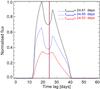 |
Fig. 5 Asymmetric case for a disk-like BLR such as 3C 120 (i = 10°, Rmin = 22 light days, Rmax = 28 light days, vmax = 2850 km s-1). The dotted lines show the time-delay function of the entire BLR (black), the BLR part outside of the filter (red), and the BLR part inside the filter (blue). The centroids of the respective curves are plotted by the vertical solid lines, which virtually coincide. |
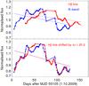 |
Fig. 6 Light curves of 3C 120 in B (blue) and Hβ (red), normalised to their mean. Top: the thin dotted lines represent the long-term trend quantified by a linear fit to the light curves. The long-term trends of B and Hβ appear to differ because a non-variable flux contribution in the Hβ light curve. Bottom: after determining and subtracting the non-variable flux in the Hβ light curve (C ~ 25%) and re-normalisation, the long-term trends agree. For visual purposes we shifted the Hβ light curve by an estimated lag time of 25 days. |
4. BLR geometry of 3C 120 from light curve modelling
The aim is to distinguish between a spherical and a disk-like BLR geometry by means of light curve modelling. Figure 6 (top) shows the B band and Hβ light curves (derived using 7 5 apertures).
The light curves are well sampled and rich in features. The B band light curve was corrected for host-galaxy contributions (see Paper I), and hence essentially represents the pure AGN light curve, which was used in the modelling as triggering input for the simulations. The Hβ light curve was constructed from the [OIII] NB light curve by essentially correcting via the V band light curve for continuum contributions (Paper I). This V band correction may be not accurate enough, and thus the resulting Hβ light curve may still contain non-variable contributions, for instance from the narrow-line region. To use this Hβ light curve as a tracer for the BLR echo, these contributions need to be removed (Sect. 4.1). The reason is that otherwise the amplitude of the modelled echo becomes always too large compared with the amplitude of the observed echo, which prevents a reliable model fit. Another concern is the gap in observational data points between days 75 and 95, which we consider in Sect. 4.2.
4.1. Correcting the Hβ light curve for non-variable contributions
To determine the potential non-variable contribution to the Hβ light curve, we performed a long-term trend analysis. The BLR size of ~25 light days is smaller than the duration of the monitoring campaign. Thus, on the long time-scale (~150 days) both B band and Hβ light curves should show the same long-term trend, but this is not the case in the original data (Fig. 6, top), which indicates an additional contribution to the Hβ light curve. After subtracting a suitably scaled non-variable contribution (C ~ 25%) from the Hβ light curve and subsequently re-normalising the long-term trends agree (Fig. 6, bottom).
Because the transfer function is not a δ-function, but spread over ~25 days, the time span of 150 days might be too short to apply the long-term trend correction above. Therefore, we derived the correction factor C of the non-variable contribution to the Hβ light curve in an alternative way. For a grid of subtracted constant contributions (C between 0% and 50%) we applied the model fitting and compared the reduced chi-square values. The best fits were obtained for C ~ 25% (Fig. 7).
The perfect agreement of C ~ 25% derived by both the long-term trend and the fitting process gives us confidence that any non-variable continuum in the Hβ light curve is well corrected for. Thus, we are confident to have obtained the proper amplitude scaling between the triggering B band variations and those of the Hβ echo.
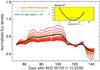 |
Fig. 7 Hβ light curves of 3C 120 with different non-variable contributions C between 0% and 50% subtracted and re-normalised (red). The best model fit is shown in black and the best corresponding data in green. The inset shows the reduced chi-square as a function of C. The best chi-square is for C ~ 25%, perfectly consistent with the C-value from the long-term trend analysis in Fig. 6. |
4.2. Applying SPEAR to bridge the observational gap
Despite the dense sampling of two days (median over six months), the observed PRM light curves have a gap of 20 days between December 2009 and January 2010 (days 75 to 95 in Fig. 6, top). These gaps constitute about 20/150 ~ 14%, i.e. a small fraction, of the monitoring. So far, we have linearly interpolated the gaps and obtained good fit results.
On the other hand, linear interpolation may have missed important variation features during the gaps. It has be shown that the AGN continuum variability can be reproduced by a damped random walk (DRW) process (Vio et al. 1992; Kelly et al. 2009; MacLeod et al. 2012). To check for consistency with stochastic models, we interpolated the continuum applying the code stochastic process estimation for AGN reverberation (SPEAR; Zu et al. 2011) – similar to what we did in Paper II. Figure 8 shows the light curve models obtained with SPEAR. They do not differ much from the interpolated light curves (Fig. 6, top). In the gaps the difference between the SPEAR and the interpolated light curves is lower than 5% and ~7 times lower than the overall variability amplitues (35%). Because of the small difference between the data and the SPEAR model light curves, and to avoid to fitting a BLR model to a light curve that itself is only a modelled curve, we decided to use the interpolated data light curves for the subsequent modelling of the BLR.
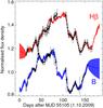 |
Fig. 8 Interpolated continuum and Hβ light curves. The solid red and blue lines show the Hβ and continuum models estimated by SPEAR. The red and blue areas (enclosed by the dashed line) represent the expected variance about the mean light curve model obtained with SPEAR. The Hβ light curve (black dots) is vertically shifted with respect to the continuum light curve (black dots) for clarity. |
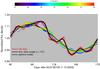 |
Fig. 9 Hβ and best-fit model light curves of 3C 120. The interpolated Hβ light curve is shown with red crosses. Note the sharp drop of the light curve at days ~110 and ~130 as well as the sharp feature at days ~150 and the strong rise at day ~170. Both the spherical BLR model (black dotted line) and the inclined thin disks (i = 45° blue solid line, i = 60° green solid line) fail in fitting these sharp variation features. The features are best fitted by a thin-disk BLR model with inclination i = 10° (black solid line). Already at i = 20° (violet solid line) the thin disk fit yields a poorer chi-square. The light curves are shown only after the initial settling-down phase (~60 days), to account for the unknown continuum light curve before day zero. |
4.3. Results and discussion
We used the host-subtracted B band light curve as the one that trigger AGN continuum light curve. We created echo model light curves, by convolving the AGN continuum light curve with the time-delay function for a spherical BLR and for thin Kepler disks at a range of inclinations. We compared the echo model light curves with the Hβ light curve. Figure 9 shows the simulation results. Particularly important are the two pronounced sharp features in the Hβ light curve, for instance the sudden declines at days ~110 and ~130. Even the best spherical fit does not reproduce these sharp features well, which makes a spherical BLR for 3C 120 highly unlikely. The same holds for the strongly inclined thin disks i> 40°. The best fit is a thin-disk BLR model with an inclination i = 10°, which well reproduces the features of the Hβ light curve; this provides strong evidence in favour of a disk-like BLR in 3C 120. From the chi-square analysis we obtain an inclination of i = 10° ± 4° for a thin-disk BLR model with an extension from 22 to 28 light days.
As a refinement of the thin disks, we also modelled thick-disk geometries with a range of covering angles. Our thick disks are simply the superposition of several disks that cover a range of inclinations. For instance, a thick disk with mean i = 10° and a covering half-angle α = 10° is composed of thin disks with 0°<i< 20°. The best chi-square of the thick-disk model yields the same extent from 22 to 28 light days as the thin disk model, but a slightly different inclination of i = 5° ± 6°, and a covering half-angle α = 10° ± 15°. The chi-square performance for i and α is shown in Fig. 10. To estimate the i and α uncertainties σi = 6° and σα = 15° we used the chi-square contours at χ2 = 5, i.e. at five times the minimum chi-square values.
The value σα = 15° appears to be relatively high and, for thick disks, rates an orbit at inclination i = + 20° as good, while it is rejected for a thin-disk fit (Fig. 9). We suggest that the relatively high σα = 15° arises because the fits of our thick disks become degenerate for nearly face-on orbits. For instance, a thick disk at mean i = + 10° and α = 20° contains – among others – two orbits one at i = + 30° and one at i = − 10°. Because χ2 does not distinguish between an orbit at i = + 10° and one at i = − 10°, the excellent i = − 10° orbit will counterbalance the poor contribution of the i = + 30° orbit. Nevertheless, the results favour a nearly face-on and rather thin disk as the best-fit solution for 3C 120.
Proper-motion studies of the superluminal radio jet of 3C 120 revealed that the highest apparent velocity is around 6c (Gómez et al. 2001; Walker et al. 2001), which allows a largest jet-viewing angle of 20° relative to the line of sight (Marscher et al. 2002). More recently, and through modelling Very Long Baseline Array (VLBA) observations, Agudo et al. (2012) estimated a jet-angle inclination of ~16°. If the jet axis is aligned with the normal vector of both the accretion disk and the BLR disk (Bardeen & Petterson 1975), the inclination values obtained from radio data are nicely consistent with our BLR inclination.
By modelling detailed spectroscopic reverberation mapping and velocity-delay maps of 3C 120, albeit with softer light curve features than seen in our data, Grier et al. (2013) and Kollatschny et al. (2014) also found evidence for a disk-like BLR, but did not specify the parameters. Remarkably, our results were obtained without explicit velocity information, but under the assumption that the BLR is essentially virialised. The light curves do not depend on the velocity of the BLR clouds, but on the location of the clouds, hence the BLR shape, which is quasi-static on the 25 day time scale considered here. The velocity information is then only needed to distinguish between a Keplerian rotation and other kinds of cloud movement such as in- or outflow, or turbulence. This explains why it is possible – under favourable conditions as in our case of 3C 120 – to infer the BLR shape even from photometric reverberation data.
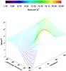 |
Fig. 10 Distribution of reduced χ2 values for inclination i and covering half-angle α of disk-like BLR models for 3C 120. The inclination starts at i = 5° (and not at i = 0°), and the grid is in steps of 3° for both i and α. The black crossed square marks the place of the minimum χ2 found at i = 5° and α = 10°. The inner and outer radius of the disks is 22 days and 28 days, respectively. |
5. Central black hole mass and the geometry scaling factor for 3C 120
If 3C 120 has a nearly face-on disk-like BLR geometry with i ~ 10°, the geometry-scaling factor f may be much higher than the commonly used average value f = 5.5 (Onken et al. 2004), which in consequence may result in a much larger black hole mass MBH. While it is not possible to determine MBH with high precision from PRM data and single-epoch spectroscopy alone, we here discuss the implications of a face-on disk-like BLR geometry, which are of widespread relevance.
Spectroscopic reverberation mapping is the only way to provide reasonably accurate MBH estimates for AGN via the virial theorem: 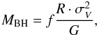 (1)where σV is the emission-line velocity dispersion (assuming Keplerian orbits of the BLR clouds), R = c·τ is the BLR size, and the factor f depends on the – so far unknown – geometry and kinematics of the BLR (Peterson et al. 2004 and references therein). RM also enables rough MBH estimates from single-epoch spectra through the use of the BLR size-luminosity
  relationship (Koratkar & Gaskell 1991; Kaspi et al. 1996; Wandel et al. 1999; McGill et al. 2008; Vestergaard & Peterson 2006; Vestergaard et al. 2011). By assuming that AGNs and quiescent galaxies follow the same MBH–σ∗ relationship, Onken et al. (2004) have shown that the scaling factor (f) has an average value of 5.5, if the velocity width is determined by considering the second moment of the line profile (σV) rather than the FWHM (VFWHM). Subsequent studies (based on the method established by Onken et al. 2004) have shown that the intrinsic scatter of the scaling factor f is about 0.4 dex (Collin et al. 2006; Woo et al. 2010; Greene et al. 2010; Graham et al. 2011), indicating that the scaling factor is a crucial source of uncertainties in determining black hole masses through the RM method or single-epoch spectra (Woo et al. 2010).
A different approach for estimating MBH is by means of the observed gravitational redshift of high-ionization emission lines (Netzer 1977; Gaskell 1982; Peterson et al. 1985; Zheng & Sulentic 1990; Kollatschny 2003a). Certainly, this technique requires high spectral resolution monitoring to detect the small redshift, for instance from the rms spectra, that is from the variable portion of the broad emission-lines. In the pioneering study of Mrk110, Kollatschny (2003a) estimated a gravitational mass of 14 ± 3 × 10⁷ M⊙, which is higher than the 2.5 ± 6 × 10⁷ M⊙ (Peterson et al. 2004) obtained by spectroscopic RM assuming a scaling factor f = 5.5. Kollatschny found evidence for a disk-like BLR with inclination i ~ 21°.
If 3C 120 has a nearly face-on disk-like BLR geometry with i ~ 10°, this results in a value  (ranging between 20 and 180 if the inclination errors are taken into account). This value is about eight times higher than the statistical value f = 5.5 obtained by Onken et al. (2004). For 3C 120, Peterson et al. (2004) determined a virial mass Mvirial = MBH/f = 10.1 ± 4 M⊙, while Grier et al. (2012) found Mvirial = 12.2 ± 1.2 × 10⁶ M⊙. In Paper I we estimated a virial mass Mvirial = 10 ± 5 × 10⁶ M⊙. Using as a conservative approach the lowest Mvirial = 10 × 106 M⊙ and the new derived scaling factor f = 46, the resulting black hole mass of 3C 120 is MBH = 460 × 106 M⊙. Figure 11 shows the position of 3C 120 in the MBH − σ∗ diagram. The data are taken from Onken et al. (2004, their Table 3). In all cases, MBH has been calculated using the velocity dispersion (Eq. (4) of Peterson et al. 2004), and with the assumption that the line width is dominated by Keplerian motion. This means that the data are treated in a homogeneous and comparable way. Figure 11 also shows the black hole mass obtained for Mrk110 via gravitational redshift (Kollatschny 2003b). The objects Mrk110 and 3C 120 clearly lie above the regression line for quiescent galaxies.
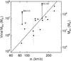 |
Fig. 11 MBH–σ∗ relationship from Onken et al. (2004) using data of Peterson et al. (2004) (black dots). The black arrows show the positional shift of 3C 120 and Mrk110 with respect to the previous ones from Peterson et al. (2004). The solid line is the best-fit slope (case F02) from Onken et al. (2004). |
To understand the overly massive black holes of Mrk110 and 3C 120, we considered three potentially scenarios.
-
i)
If the broad-line profiles in AGN are contaminated by turbulence or outflowing winds in the line-emitting region (Murray & Chiang 1997; Kollatschny & Zetzl 2013), the emission-line velocity dispersion (σV) may be increased, leading to an overestimate of the black hole mass by means of the virial product. However, this does not explain the case of Mrk110.
-
ii)
If AGNs have (bipolar) outflows (Kollatschny 2003b; Denney et al. 2009), the host galaxy bulge will get a hole, hence will not be isotropic. If such an AGN/bulge system is seen close to pole-on, the bulge will appear with a flattened stellar distribution and therefore the stellar bulge velocity dispersion (σ∗) will be lower (than that of a quiescent galaxy with a more isotropic bulge). However, it remains an open question, whether σ∗ can be diminished by the factor 2−3 needed to bring 3C 120 and Mrk110 back on the MBH–σ∗ relation.
-
iii)
If we consider two galaxies with the same bulge mass (Mbulge), but with a different black hole mass (MBH), the sphere of influence of the galaxy with larger MBH will be larger and may lead to stronger or more frequent activity, in consequence, leading to an enhanced black hole growth relative to the bulge growth. Thus, the assumption that AGNs and quiescent galaxies follow the same MBH − σ∗ relationship may not be valid in general.
6. Summary and conclusions
We have investigated two aspects of the efficient method of photometric reverberation mapping.
Firstly we examined how the determination of the mean BLR size is affected when the broad emission-line is not fully covered by the chosen narrow-band filter. By modelling a range of configurations and assuming circular Keplerian orbits, we found that for reasonable line-width band-pass configurations the possible biases for the mean BLR size are lower than a few percent. Asymmetric cutting of emission line by the filter has probably even weaker effects. In view of the overall measurements errors of typically more than 10%, any bias in the mean BLR size derived from narrow-band photometric reverberation mapping appears to be negligible.
Secondly, we modelled the feature-rich photometric reverberation light curves of 3C 120 to determine the basic geometry of the BLR, whether it is spherical or disk-like. The narrow-band light curves cover the central and the blue part of the Hβ line, but miss the red wing. Guided by velocity-resolved spectroscopic reverberation data, we assumed that the BLR, as seen in our narrow-band light curves, is dominated by the Keplerian motion and not by in- or outflows nor by turbulence. While a spherical BLR model does not fit the PRM observations, a thin-disk BLR model that extends from 22 to 28 light days and has an inclination i = 10 ± 4 degrees excellently reproduced the Hβ light curve of 3C 120. A similar fit quality was reached for a moderately thick-disk BLR model with inclination of i = 5° ± 6°, and a covering half-angle α = 10° ± 15°.
Finally, if this result of a disk-like BLR also holds for Seyfert galaxies in general, the determination of the f-factor used in black hole mass calculations can be remarkably improved. The current data already indicate that the black hole of 3C 120 is more massive than the MBH–σ∗ relation for quiescent galaxies. While this needs to be corroborated with future data, it appears to be consistent with findings from the gravitational redshift of Mrk110 and with overly massive black holes in high-redshift AGNs.
Acknowledgments
This work is supported by the Nordrhein-Westfälische Akademie der Wissenschaften und der Künste in the framework of the academy program of the Federal Republic of Germany and the state Nordrhein-Westfalen and by the Deutsche Forschungsgemeinschaft (DFG HA3555/12-1 and KO857/32-1). The observations on Cerro Armazones benefitted from the care of the guardians Hector Labra, Gerardo Pino, Roberto Munoz, and Francisco Arraya. This research has made use of the NASA/IPAC Extragalactic Database (NED) which is operated by the Jet Propulsion Laboratory, California Institute of Technology, under contract with the National Aeronautics and Space Administration. This research has made use of the SIMBAD database, operated at CDS, Strasbourg, France. We thank the anonymous referee for constructive comments.
References
- Agudo, I., Gómez, J. L., Casadio, C., Cawthorne, T. V., & Roca-Sogorb, M. 2012, ApJ, 752, 92 [NASA ADS] [CrossRef] [Google Scholar]
- Baldwin, J., Ferland, G., Korista, K., & Verner, D. 1995, ApJ, 455, L119 [NASA ADS] [CrossRef] [Google Scholar]
- Bardeen, J. M., & Petterson, J. A. 1975, ApJ, 195, L65 [NASA ADS] [CrossRef] [Google Scholar]
- Bentz, M. C., Peterson, B. M., Netzer, H., Pogge, R. W., & Vestergaard, M. 2009, ApJ, 697, 160 [Google Scholar]
- Blandford, R. D., & McKee, C. F. 1982, ApJ, 255, 419 [NASA ADS] [CrossRef] [EDP Sciences] [Google Scholar]
- Brewer, B. J., Treu, T., Pancoast, A., et al. 2011, ApJ, 733, L33 [NASA ADS] [CrossRef] [Google Scholar]
- Bottorff, M., Korista, K. T., Shlosman, I., & Blandford, R. D. 1997, ApJ, 479, 200 [NASA ADS] [CrossRef] [Google Scholar]
- Chelouche, D. 2013, ApJ, 772, 9 [NASA ADS] [CrossRef] [Google Scholar]
- Chelouche, D., & Daniel, E. 2012, ApJ, 747, 62 [NASA ADS] [CrossRef] [Google Scholar]
- Chelouche, D., & Zucker, S. 2013, ApJ, 769, 124 [NASA ADS] [CrossRef] [Google Scholar]
- Chelouche, D., Daniel, E., & Kaspi, S. 2012, ApJ, 750, L43 [NASA ADS] [CrossRef] [Google Scholar]
- Cherepashchuk, A. M., & Lyutyi, V. M. 1973, Astrophys. Lett., 13, 165 [NASA ADS] [Google Scholar]
- Collin, S., Kawaguchi, T., Peterson, B. M., & Vestergaard, M. 2006, A&A, 456, 75 [NASA ADS] [CrossRef] [EDP Sciences] [Google Scholar]
- Denney, K. D., Peterson, B. M., Pogge, R. W., et al. 2009, ApJ, 704, L80 [NASA ADS] [CrossRef] [Google Scholar]
- Drouart, G., De Breuck, C., Vernet, J., et al. 2014, ApJ, 566, A53 [Google Scholar]
- Edri, H., Rafter, S. E., Chelouche, D., Kaspi, S., & Behar, E. 2012, ApJ, 756, 73 [NASA ADS] [CrossRef] [Google Scholar]
- Elvis, M. 2000, ApJ, 545, 63 [NASA ADS] [CrossRef] [Google Scholar]
- Gaskell, C. M. 1982, ApJ, 263, 79 [NASA ADS] [CrossRef] [Google Scholar]
- Gaskell, C. M., & Sparke, L. S. 1986, ApJ, 305, 175 [NASA ADS] [CrossRef] [Google Scholar]
- Gómez, J.-L., Marscher, A. P., Alberdi, A., Jorstad, S. G., & Agudo, I. 2001, ApJ, 561, L161 [NASA ADS] [CrossRef] [Google Scholar]
- Graham, A. W., Onken, C. A., Athanassoula, E., & Combes, F. 2011, MNRAS, 412, 2211 [NASA ADS] [CrossRef] [Google Scholar]
- Greene, J. E., Peng, C. Y., & Ludwig, R. R. 2010, ApJ, 709, 937 [Google Scholar]
- Grier, C. J., Peterson, B. M., Pogge, R. W., et al. 2012, ApJ, 755, 60 [NASA ADS] [CrossRef] [Google Scholar]
- Grier, C. J., Peterson, B. M., Horne, K., et al. 2013, ApJ, 764, 47 [NASA ADS] [CrossRef] [Google Scholar]
- Haas, M., Chini, R., Ramolla, M., et al. 2011, A&A, 535, A73 [NASA ADS] [CrossRef] [EDP Sciences] [Google Scholar]
- Horne, K. 2003, Proc. SPIE, 4854, 262 [NASA ADS] [CrossRef] [Google Scholar]
- Kaspi, S., Smith, P. S., Maoz, D., Netzer, H., & Jannuzi, B. T. 1996, ApJ, 471, L75 [NASA ADS] [CrossRef] [Google Scholar]
- Kaspi, S., Smith, P. S., Netzer, H., et al. 2000, ApJ, 533, 631 [NASA ADS] [CrossRef] [Google Scholar]
- Kelly, B. C., Bechtold, J., & Siemiginowska, A. 2009, ApJ, 698, 895 [Google Scholar]
- Kollatschny, W. 2003a, A&A, 412, L61 [NASA ADS] [CrossRef] [EDP Sciences] [Google Scholar]
- Kollatschny, W. 2003b, A&A, 407, 461 [NASA ADS] [CrossRef] [EDP Sciences] [Google Scholar]
- Kollatschny, W., & Zetzl, M. 2011, Nature, 470, 366 [NASA ADS] [CrossRef] [Google Scholar]
- Kollatschny, W., & Zetzl, M. 2013, A&A, 549, A100 [NASA ADS] [CrossRef] [EDP Sciences] [Google Scholar]
- Kollatschny, W., Ulbrich, K., Zetzl, M., Kaspi, S., & Haas, M. 2014, A&A, 566, A106 [NASA ADS] [CrossRef] [EDP Sciences] [Google Scholar]
- Konigl, A., & Kartje, J. F. 1994, ApJ, 434, 446 [NASA ADS] [CrossRef] [Google Scholar]
- Koratkar, A. P., & Gaskell, C. M. 1991, Variability of Active Galactic Nuclei (Cambridge University Press), 339 [Google Scholar]
- Krolik, J. H. 2001, ApJ, 551, 72 [NASA ADS] [CrossRef] [Google Scholar]
- Lyutyi, V. M., & Cherepashchuk, A. M. 1972, Astronomicheskij Tsirkulyar, 688, 1 [NASA ADS] [Google Scholar]
- MacLeod, C. L., Ivezić, Ž., Sesar, B., et al. 2012, ApJ, 753, 106 [NASA ADS] [CrossRef] [Google Scholar]
- Marscher, A. P., Jorstad, S. G., Gómez, J.-L., et al. 2002, Nature, 417, 625 [NASA ADS] [CrossRef] [PubMed] [Google Scholar]
- McGill, K. L., Woo, J.-H., Treu, T., & Malkan, M. A. 2008, ApJ, 673, 703 [NASA ADS] [CrossRef] [Google Scholar]
- Murray, N., & Chiang, J. 1997, ApJ, 474, 91 [NASA ADS] [CrossRef] [Google Scholar]
- Netzer, H. 1977, MNRAS, 181, 89P [NASA ADS] [CrossRef] [Google Scholar]
- Onken, C. A., & Peterson, B. M. 2002, ApJ, 572, 746 [NASA ADS] [CrossRef] [Google Scholar]
- Onken, C. A., Ferrarese, L., Merritt, D., et al. 2004, ApJ, 615, 645 [NASA ADS] [CrossRef] [Google Scholar]
- Pancoast, A., Brewer, B. J., & Treu, T. 2011, ApJ, 730, 139 [NASA ADS] [CrossRef] [Google Scholar]
- Pancoast, A., Brewer, B. J., Treu, T., et al. 2012, ApJ, 754, 49 [NASA ADS] [CrossRef] [Google Scholar]
- Peterson, B. M. 1993, PASP, 105, 247 [NASA ADS] [CrossRef] [Google Scholar]
- Peterson, B. M., & Wandel, A. 1999, ApJ, 521, L95 [NASA ADS] [CrossRef] [Google Scholar]
- Peterson, B. M., Meyers, K. A., Carpriotti, E. R., et al. 1985, ApJ, 292, 164 [NASA ADS] [CrossRef] [Google Scholar]
- Peterson, B. M., Ferrarese, L., Gilbert, K. M., et al. 2004, ApJ, 613, 682 [NASA ADS] [CrossRef] [Google Scholar]
- PozoNuñez, F., Ramolla, M., Westhues, C., et al. 2012, A&A, 545, A84 [NASA ADS] [CrossRef] [EDP Sciences] [Google Scholar]
- Pozo Nuñez, F., Westhues, C., Ramolla, M., et al. 2013, A&A, 552, A1 [NASA ADS] [CrossRef] [EDP Sciences] [Google Scholar]
- Vestergaard, M., & Peterson, B. M. 2006, ApJ, 641, 689 [NASA ADS] [CrossRef] [Google Scholar]
- Vestergaard, M., Denney, K., Fan, X., et al. 2011, Narrow-Line Seyfert 1 Galaxies and their Place in the Universe, Milano, Italy, Proc. of Science [Google Scholar]
- Vio, R., Cristiani, S., Lessi, O., & Provenzale, A. 1992, ApJ, 391, 518 [NASA ADS] [CrossRef] [Google Scholar]
- Walker, R. C., Benson, J. M., Unwin, S. C., et al. 2001, ApJ, 556, 756 [NASA ADS] [CrossRef] [Google Scholar]
- Wandel, A., Peterson, B. M., & Malkan, M. A. 1999, ApJ, 526, 579 [NASA ADS] [CrossRef] [Google Scholar]
- Wang, R., Carilli, C. L., Neri, R., et al. 2010, ApJ, 714, 699 [NASA ADS] [CrossRef] [Google Scholar]
- Welsh, W. F., & Horne, K. 1991, ApJ, 379, 586 [NASA ADS] [CrossRef] [Google Scholar]
- Wills, B. J., & Browne, I. W. A. 1986, ApJ, 302, 56 [NASA ADS] [CrossRef] [Google Scholar]
- Woo, J.-H., Treu, T., Barth, A. J., et al. 2010, ApJ, 716, 26 [Google Scholar]
- Zheng, W., & Sulentic, J. W. 1990, ApJ, 350, 512 [NASA ADS] [CrossRef] [Google Scholar]
- Zu, Y., Kochanek, C. S., & Peterson, B. M. 2011, ApJ, 735, 80 [NASA ADS] [CrossRef] [Google Scholar]
All Figures
|
Fig. 1 Symmetric case of a thin disk-like BLR geometry (i = 45°, Rmin = 20 light days, Rmax = 30 light days, vmax = 3700 km s-1). Top: a rectangular filter (dotted line) is symmetrically centred on the spectral line (thick solid line); the parts of the line that are cut off by the filter are shaded in red. Bottom: BLR areas inside (black) and outside (red) of the filter. If a disk-like BLR-model with Keplerian orbits is assumed, the red shaded areas with the highest apparent velocity are cut off by the filter. |
| In the text | |
|
Fig. 2 Response of the BLR to a single light-pulse. The BLR is modelled as a thin circular Keplerian-disk. The dotted curves show the time-delay function of the entire BLR (black), the BLR part outside of the NB (red dotted line), and the BLR part inside of the NB (blue dashed line). The response of the entire emission line (black) can be separated into a part contained by the NB and a part outside the NB. The solid vertical lines mark the centroids of the filter answers (i.e. the mean time lag). The difference between the blue and the black centroid is the response (echo) bias. The value of the measured echo (blue) is higher than that of the real one (black). Thus, cutting line wings will (marginally) increase the mean time lag. |
| In the text | |
|
Fig. 3 Dependence of the time-lag over-estimate for a thin-disk BLR at inclination 45°. For each value of rmax/rmin, the curve shows the lag over-estimate as a function of line cut, here expressed as light lost. |
| In the text | |
|
Fig. 4 Asymmetric case for a disk-like BLR such as 3C 120 (i = 10°, Rmin = 22 light days, Rmax = 28 light days, vmax = 2850 km s-1). Top: NB filter ([OIII]λ 5007 Å, dotted line) and emission-line profile of the BLR (Hβ, thick solid line). The filter essentially covers the complete blue half of the Hβ line, as is the case for 3C 120. Bottom: BLR areas inside (black) and outside (coloured) of the NB filter. The colour-coding (blue, green, red) indicates a line transmission of about 50%, 20%, and 0%. |
| In the text | |
|
Fig. 5 Asymmetric case for a disk-like BLR such as 3C 120 (i = 10°, Rmin = 22 light days, Rmax = 28 light days, vmax = 2850 km s-1). The dotted lines show the time-delay function of the entire BLR (black), the BLR part outside of the filter (red), and the BLR part inside the filter (blue). The centroids of the respective curves are plotted by the vertical solid lines, which virtually coincide. |
| In the text | |
|
Fig. 6 Light curves of 3C 120 in B (blue) and Hβ (red), normalised to their mean. Top: the thin dotted lines represent the long-term trend quantified by a linear fit to the light curves. The long-term trends of B and Hβ appear to differ because a non-variable flux contribution in the Hβ light curve. Bottom: after determining and subtracting the non-variable flux in the Hβ light curve (C ~ 25%) and re-normalisation, the long-term trends agree. For visual purposes we shifted the Hβ light curve by an estimated lag time of 25 days. |
| In the text | |
|
Fig. 7 Hβ light curves of 3C 120 with different non-variable contributions C between 0% and 50% subtracted and re-normalised (red). The best model fit is shown in black and the best corresponding data in green. The inset shows the reduced chi-square as a function of C. The best chi-square is for C ~ 25%, perfectly consistent with the C-value from the long-term trend analysis in Fig. 6. |
| In the text | |
|
Fig. 8 Interpolated continuum and Hβ light curves. The solid red and blue lines show the Hβ and continuum models estimated by SPEAR. The red and blue areas (enclosed by the dashed line) represent the expected variance about the mean light curve model obtained with SPEAR. The Hβ light curve (black dots) is vertically shifted with respect to the continuum light curve (black dots) for clarity. |
| In the text | |
|
Fig. 9 Hβ and best-fit model light curves of 3C 120. The interpolated Hβ light curve is shown with red crosses. Note the sharp drop of the light curve at days ~110 and ~130 as well as the sharp feature at days ~150 and the strong rise at day ~170. Both the spherical BLR model (black dotted line) and the inclined thin disks (i = 45° blue solid line, i = 60° green solid line) fail in fitting these sharp variation features. The features are best fitted by a thin-disk BLR model with inclination i = 10° (black solid line). Already at i = 20° (violet solid line) the thin disk fit yields a poorer chi-square. The light curves are shown only after the initial settling-down phase (~60 days), to account for the unknown continuum light curve before day zero. |
| In the text | |
|
Fig. 10 Distribution of reduced χ2 values for inclination i and covering half-angle α of disk-like BLR models for 3C 120. The inclination starts at i = 5° (and not at i = 0°), and the grid is in steps of 3° for both i and α. The black crossed square marks the place of the minimum χ2 found at i = 5° and α = 10°. The inner and outer radius of the disks is 22 days and 28 days, respectively. |
| In the text | |
|
Fig. 11 MBH–σ∗ relationship from Onken et al. (2004) using data of Peterson et al. (2004) (black dots). The black arrows show the positional shift of 3C 120 and Mrk110 with respect to the previous ones from Peterson et al. (2004). The solid line is the best-fit slope (case F02) from Onken et al. (2004). |
| In the text | |
Current usage metrics show cumulative count of Article Views (full-text article views including HTML views, PDF and ePub downloads, according to the available data) and Abstracts Views on Vision4Press platform.
Data correspond to usage on the plateform after 2015. The current usage metrics is available 48-96 hours after online publication and is updated daily on week days.
Initial download of the metrics may take a while.