| Issue |
A&A
Volume 567, July 2014
|
|
|---|---|---|
| Article Number | A8 | |
| Number of page(s) | 8 | |
| Section | Planets and planetary systems | |
| DOI | https://doi.org/10.1051/0004-6361/201423795 | |
| Published online | 04 July 2014 | |
Observed spectral energy distribution of the thermal emission from the dayside of WASP-46b⋆,⋆⋆,⋆⋆⋆
1 Purple Mountain Observatory & Key Laboratory for Radio Astronomy, Chinese Academy of Sciences, 2 West Beijing Road, 210008 Nanjing, PR China
e-mail: guochen@pmo.ac.cn
2 University of Chinese Academy of Sciences, 19A Yuquan Road, 100049 Beijing, PR China
3 Max Planck Institute for Astronomy, Königstuhl 17, 69117 Heidelberg, Germany
4 Astrophysics Group, University of Exeter, Stocker Road, EX4 4 QL Exeter, UK
5 Institut für Astrophysik, Friedrich-Hund-Platz 1, 37077 Göttingen, Germany
Received: 12 March 2014
Accepted: 22 May 2014
Aims. We aim to construct a spectral energy distribution (SED) for the emission from the dayside atmosphere of the hot Jupiter WASP-46b and to investigate its energy budget.
Methods. We observed a secondary eclipse of WASP-46b simultaneously in the g′r′i′z′JHK bands using the GROND instrument on the MPG/ESO 2.2 m telescope. Eclipse depths of the acquired light curves were derived to infer the brightness temperatures at multibands that cover the SED peak.
Results. We report the first detection of the thermal emission from the dayside of WASP-46b in the K band at 4.2σ level and tentative detections in the H (2.5σ) and J (2.3σ) bands, with flux ratios of 0.253 +0.063-0.060%, 0.194 ± 0.078%, and 0.129 ± 0.055%, respectively. The derived brightness temperatures (2306 +177-187 K, 2462 +245-302 K, and 2453 +198-258 K, respectively) are consistent with an isothermal temperature profile of 2386 K, which is significantly higher than the dayside-averaged equilibrium temperature, indicative of very poor heat redistribution efficiency. We also investigate the tentative detections in the g′r′i′ bands and the 3σ upper limit in the z′ band, which might indicate the existence of reflective clouds if these tentative detections do not arise from systematics.
Key words: stars: individual: WASP-46 / planets and satellites: individual: WASP-46b / planets and satellites: atmospheres / planetary systems / techniques: photometric
Based on observations collected with the Gamma Ray burst Optical and Near-infrared Detector (GROND) on the MPG/ESO 2.2 m telescope at the La Silla Observatory, Chile. Program 088.A-9016 (PI: Chen).
Appendix A is available in electronic form at http://www.aanda.org
Photometric time series are only available at the CDS via anonymous ftp to cdsarc.u-strasbg.fr (130.79.128.5) or via http://cdsarc.u-strasbg.fr/viz-bin/qcat?J/A+A/567/A8
© ESO, 2014
1. Introduction
Observation of a hot-Jupiter secondary eclipse is one of the most efficient ways to characterize exoplanet atmospheres. The signals from the dayside atmosphere can be discerned through the comparison between in-eclipse and out-of-eclipse measurements. Such observations have been performed on dozens of exoplanets by the Spitzer and Hubble space telescopes in the mid-infrared and 1.1–1.7 μm wavelength range, respectively (see the reviews by Seager & Deming 2010; Madhusudhan et al. 2014, and references therein). Chemical compositions, such as H2O, CO, CO2, and CH4, can be investigated based on multiwavelength data with the help of an atmospheric retrieval modeling technique (e.g., Madhusudhan & Seager 2009; Lee et al. 2012; Line et al. 2012). Existence of thermal inversions is inferred using the emission behavior of these molecules (Fortney et al. 2008; Burrows et al. 2008; Madhusudhan & Seager 2010). On the other hand, results from ground-based near-infrared (NIR) observations have emerged rapidly during the past three years (e.g., Croll et al. 2011; Cáceres et al. 2011; de Mooij et al. 2011; Gillon et al. 2012; Zhao et al. 2012a,b; Deming et al. 2012; Crossfield et al. 2012; de Mooij et al. 2013; Wang et al. 2013; O’Rourke et al. 2014; Chen et al. 2014a,b), providing a good complement to the wavelength ranges covered by Spitzer and Hubble. The planetary energy budget can be constrained in the NIR where the planetary spectral energy distribution (SED) peaks. The vertical temperature profile can be constrained at the lower atmospheric layers since the J, H, K bands overlap weaker molecular bands and thus probe deeper than the mid-infrared bands.
WASP-46b is a hot Jupiter orbiting a G6V star every 1.43 days (Anderson et al. 2012). Its mass and radius were deduced to be 2.10 MJup and 1.31 RJup, resulting in a bulk density similar to our Jupiter. Taking the planetary radius, the orbital distance, and the stellar effective temperature into account, it is expected to be highly irradiated, with an incident flux of 1.7×10⁹ erg s-1 cm-2. This translates into an equilibrium temperature of 1654 K, assuming zero albedo and planet-wide heat redistribution. Combined with the high planet-to-star area ratio ( ), this hot Jupiter is a favorable target for detecting the thermal emission from its dayside atmosphere. Anderson et al. (2012) also found that its host star is active, since it has a 16-day rotational modulation and weak Ca ii H+K emission. The stellar activity might prevent a thermal inversion in the upper atmosphere, given the hypothesis that the high UV flux could destroy the high-altitude compounds responsible for the formation of temperature inversion (Knutson et al. 2010).
We aim at detecting the dayside emission of WASP-46b by observing its secondary eclipse simultaneously in seven bands. We expect to construct an SED for its dayside emission, to study its energy budget, and to obtain first insight into its temperature profile. This work belongs to our project that characterizes hot-Jupiter atmospheres using the technique of simultaneous multiband photometry, in which we have detected the thermal emission of WASP-5b in the J and K bands (Chen et al. 2014a) and the thermal emission of WASP-43b in the K band (Chen et al. 2014b).
Here we report the first detection of the thermal emission from the dayside atmosphere of WASP-46b. This paper is organized as follows: in Sect. 2 we summarize the observation and data reduction. In Sect. 3 we describe the light-curve modeling process. In Sect. 4 we present the analysis results and discuss the atmosphere delivered by our data. Finally, Sect. 5 gives the conclusions.
2. Observations and data reduction
We observed one secondary eclipse of WASP-46b using the Gamma Ray burst Optical and Near-infrared Detector (GROND; Greiner et al. 2008) mounted on the MPG/ESO 2.2 m telescope at La Silla in Chile. This imaging instrument uses dichroics to acquire data simultaneously in the Sloan g′r′i′z′ and NIR JHK bands. The optical arm employs backside-illuminated 2048 × 2048 E2V CCDs without antiblooming structures, which has a field of view (FOV) of 5.4′ × 5.4′ (0 158 per pixel). The NIR arm employs 1024 × 1024 Rockwell HAWAII-1 arrays, with an FOV of 10′ × 10′ (060 per pixel).
The secondary eclipse was observed on October 9, 2011. The observation started at 90 min before the first contact (i.e., ingress) and ended at 50 min after the last contact (i.e., egress), continuously lasting four hours, with an overall airmass below 1.40. Staring mode was adopted and no defocusing was applied. We used 30 s exposures for the optical cameras and 4.5 s exposures for the NIR cameras. The optical images were collected in fast read-out mode. The NIR images were averaged every four frames before read-out. Most of the peak pixels of the target star in the JHK bands have values around 104 ADU, while a few can rise as high as 2 × 10⁴ ADU at the end of the observation. All of these values lie below the 1% nonlinearity of the detector, thus no nonlinearity correction was applied in the subsequent calibration to avoid introducing additional noise. After accounting for the dead time caused by telescope operation and the time for file read-out and saving, we calculated an effective duty cycle of 51% and 61% for the optical and NIR bands. Since this observation started before the end of evening twilight, the sky count levels were high at the beginning and decreased quickly afterwards. After checking the relative sky variation (see Fig. 1), we discarded the first-hour data1 in the subsequent reduction and analysis. This leaves 185 and 371 frames for the optical and NIR bands.
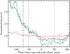 |
Fig. 1 Normalized sky level versus elapsed time. Blue, green, and red curves show the sky levels of the J, H, and K bands. For each band, all the values are normalized by its median, so as to illustrate the overall variation. Data that were acquired before the time indicated by the vertical dashed line are not included in our final analysis. Two dotted lines indicate the expected first and last contacts of the secondary eclipse based on the assumption of a circular orbit. |
The optical and NIR images were reduced following the approach described in Chen et al. (2014a,b). In brief, the calibration steps for the optical bands include bias subtraction and flat division; for the NIR bands, they are dark subtraction, readout pattern removal, and flat division. We performed aperture photometry on WASP-46 and several reference stars using the IDL routines of DAOPHOT. The reference star ensembles for each band were selected to be unsaturated and to have similar brightness to WASP-46. They were individually normalized by each one’s median flux and were then weighted combined as the composite reference. After dividing the flux of WASP-46 by that of the composite reference, we constructed the eclipse light curves that were free of common-mode systematics to the first order. We empirically selected the optimal aperture radius and sky annuli sizes by minimizing the rms of the eclipse light curves. Consistent results were found for the photometry that is derived with aperture radius and sky annulus sizes close to the optimal choice.
We extracted the UTC time stamps and centered them on the actual mid-exposure time. They were converted into BJDTDB using the IDL routines written by Eastman et al. (2010). Since the eclipse light curves show visible systematics (see the left-hand panels of Figs. 2 and 3) correlated with target location drift, seeing variation, and possibly airmass, we also collected the following auxiliary time-correlated information for the subsequent modeling process: target centroid on the detector (x, y), FWHM of the target’s PSF (sx, sy), and airmass (z).
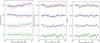 |
Fig. 2 Secondary-eclipse light curves of WASP-46b as observed with GROND in the g′r′i′z′ bands. Left panel: light curves that are normalized by the reference stars. Middle panel: baseline-corrected light curves that are binned every 10 min for display purpose. Right panel: best-fit light-curve residuals that are binned every 10 min. All the best-fit models are indicated by solid lines. |
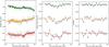 |
Fig. 3 Secondary-eclipse light curves of WASP-46b as observed with GROND in the JHK bands. Left panel: light curves that are normalized by the reference stars. Middle panel: baseline-corrected light curves that are binned every 10 min for display purpose. Right panel: best-fit light-curve residuals that are binned every 10 min. All the best-fit models are indicated by solid lines. |
3. Light-curve analysis
The reference-corrected light curves are still systematics dominated. To measure the eclipse depth from the noisy data, we chose to model the light curves using the following combination:  (1)where E(pi) is the analytic eclipse model (Mandel & Agol 2002) for a uniform disk, and the remaining component is the baseline function (BF). In the modeling process, we fit for the mid-eclipse time Tmid,occ and the planet-to-star flux ratio Fp/F⋆ in the model E(pi), along with the baseline coefficients cj in the BF. The number of cj depends on the choice of BF model vectors vj, which were empirically determined for each individual light curve. The planetary and stellar parameters needed in the model E(pi) are taken from Anderson et al. (2012), and are listed in Table 1.
We used the Markov chain Monte Carlo (MCMC) technique (e.g., Ford 2005, 2006) together with the singular-value decomposition (SVD) linear regression method to search for the best-fit values and uncertainties for the free parameters, as described in detail in Chen et al. (2014a,b, and references therein). At each MCMC step, the light-curve data were divided by a perturbed eclipse model, and then the baseline coefficients were linearly solved from the residuals by the SVD method. Since the g′r′i′z′JHK light curves were simultaneously obtained and covered the same secondary eclipse, they were forced to share the same Tmid,occ in the MCMC modeling process, while they were allowed to have wavelength-dependent Fp/F⋆. We first ran five chains of 105 links to derive an initial distribution for each parameter. Then we followed the approach of Winn et al. (2008) to account for the time-correlated red noise (for details see Chen et al. 2014a,b), which makes use of both the time-averaging method and the prayer-bead method to determine the red-noise scaling factors. The larger one was adopted as βr and was multiplied on the photometric uncertainties. Finally, we ran another five chains of 105 links on the light curves with rescaled uncertainties to derive the final best-fit values and 68.3% uncertainties for the free parameters.
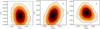 |
Fig. 4 Dependence of the measured flux ratio on the measured mid-eclipse time (converted to orbital phase) for the J (left), H (middle), and K (right) bands. Three contour levels correspond to the 1σ, 2σ, and 3σ confidence levels, respectively. |
We experimented with a set of BF models to find the one that best characterizes the systematics in each light curve. The best chosen BF models were determined based on the Bayesian information criterion (BIC; Schwarz 1978): BIC = χ2 + klog (N), where k and N refer to the number of free parameters and data points, respectively, and χ2 is derived based on the photometric uncertainties in which the red-noise effect has not been included. We extensively explored different combinations for the BF vector, including linear, quadratic, and high-order polynomials. Those with the lowest BIC were considered as the final choice. The coefficients of the best BF models are listed in Tables A.1 and A.2. Five of the top-ranked (i.e., with the lowest BIC) BF models are shown in Table A.3 for comparison. Different choices of BF model could have an impact on the derived eclipse depth. In general, BF models with high BIC produce eclipse depths that deviate from the chosen one. However, for the BF models with a BIC similar to the lowest BIC, the best-fit values for the eclipse depth, although slightly different, are generally consistent with each other within 1σ uncertainties (see Table A.3).
We also repeated the MCMC modeling process by including the eclipse duration time T58 in the light-curve model E(pi). Given the data quality, we decided to control the values of Tmid,occ and Fp/F⋆ with the Gaussian priors. We adopted the derived distributions of Tmid,occ and Fp/F⋆ from the aforementioned analysis. The derived eclipse duration time was used to analyze the orbital eccentricity.
We present the derived best-fit parameters in Tables 1 and 2 along with the adopted parameters and photometric settings. We show the light-curve modeling results in Figs. 2 and 3 and the dependence of measured eclipse depth on mid-eclipse time in Fig. 4. We illustrate the time-averaging process in Fig. 5. After the joint MCMC modeling process, we achieved a photometric precision of 844, 615, 883, 1035, 1117, 1764, and 2325 ppm in two-minute intervals in the best-fit light-curve residuals for the g′r′i′z′JHK bands, respectively. The corresponding photon noise limits in two-minute intervals are 3.2 × 10⁻⁴, 2.4 × 10⁻⁴, 3.3 × 10⁻⁴, 3.3 × 10⁻⁴, 3.4 × 10⁻⁴, 3.4 × 10⁻⁴, and 5.6 × 10⁻⁴, respectively.
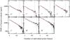 |
Fig. 5 Standard deviation of the best-fit light-curve residuals binned in different time resolutions. The vertical dashed line refers to the ingress/egress duration. The dashed red line presents the expected Poisson-like noise. The deviation above the dashed red line indicates time-correlated red noise. |
Flux ratios and other parameters from the joint analysis.
4. Results and discussion
We detect the secondary-eclipse dip in the K band with a flux ratio of 0.253  % at the 4.2σ significance level, and tentatively detect the dip in the J (2.5σ) and H (2.3σ) bands with flux ratios of 0.194 ± 0.078% and 0.129 ± 0.055%, respectively. In the optical bands, we do not detect the dip in the z′ band, while we tentatively detect the dip in the g′r′i′ bands at very low significance level.
4.1. Orbital eccentricity
The orbital eccentricity e and the argument of periastron ω are linked by the central times and the durations of both transit and eclipse, see for example, Eq. (17) and (18) in Ragozzine & Wolf (2009). The center of the secondary eclipse is expected to occur at an observed phase φ = 0.5002, if a circular orbit for WASP-46b is assumed. This calculation has accounted for the light travel time of 24.3 s in the system (Loeb 2005). From our joint analysis of the seven eclipse light curves, we derive a mid-eclipse time that deviates 9.6  minutes from this expected time, which corresponds to a corrected phase of 0.5047 ± 0.0014. This offset time corresponds to ecosω = 0.0073 ± 0.0022. In addition, we measure an eclipse duration of 0.0639
  days that is marginally shorter than the transit duration (T14 = 0.06973 days), corresponding to esinω = −0.018 ± 0.015. This calculation gives an eccentricity of
  at low significance, which is consistent with the value derived from the radial velocity data (
 ; Anderson et al. 2012). The eccentricity is consistent with zero at 2σ level. It is possible that the orbit is indeed slightly eccentric. However, we also caution that our central eclipse time and eclipse duration could be contaminated by the time-correlated systematics. To better constrain these orbital parameters, light curves with higher precision and deeper dips (i.e., higher signal-to-noise ratio) are required, for instance, from warm Spitzer.
4.2. Near-infrared thermal emission from the dayside atmosphere of WASP-46b
The derived J-, H-, K-band flux ratios of 0.129 ± 0.055%, 0.194 ± 0.078%, 0.253 % can be translated into brightness temperatures of 2453  K, 2462
 K, 2306
 K, respectively. In this calculation, we simply assumed that the planet radiates blackbody emission. We interpolated the stellar spectrum based on the Kurucz models (Kurucz 1979), using the stellar parameters Teff,⋆ = 5620 K, [Fe/H] = −0.37, and log g⋆ = 4.493 (Anderson et al. 2012). After individually integrating the planetary emission and the stellar emission over the bandpass of each filter and taking the planet-to-star area ratio () into account, we record the brightness temperature that results in the flux ratio that best matches the measured value. The derived brightness temperatures are significantly higher (~3σ) than the equilibrium temperature of 1654 ± 50 K that assumes homogeneous planet-wide redistribution of the incident heat (AB = 0 and f = 1/4). The equilibrium temperature is given by the equation
 ![\begin{equation} T_{\mathrm{eq}}=T_{\mathrm{eff,\star}}\sqrt{R_{\star}/a}[f(1-A_{\rm B})]^{1/4}, \end{equation}](/articles/aa/full_html/2014/07/aa23795-14/aa23795-14-eq132.png) (2)where AB is the Bond albedo, and f ranges from 1/4 to 2/3 (Cowan & Agol 2011). Assuming AB = 0 and f = 2/3, that is, instant re-emission of incident heat with no redistribution, the highest equilibrium temperature is calculated to be 2120 ± 67 K, which agrees with the NIR brightness temperatures at 1σ level. Therefore, if the energy excess is not of physical origin (e.g., internal energy sources), it could be explained by the large uncertainties stemming from the poor data quality. This also indicates that the energy redistribution efficiency in the dayside atmosphere is very poor.
(2)where AB is the Bond albedo, and f ranges from 1/4 to 2/3 (Cowan & Agol 2011). Assuming AB = 0 and f = 2/3, that is, instant re-emission of incident heat with no redistribution, the highest equilibrium temperature is calculated to be 2120 ± 67 K, which agrees with the NIR brightness temperatures at 1σ level. Therefore, if the energy excess is not of physical origin (e.g., internal energy sources), it could be explained by the large uncertainties stemming from the poor data quality. This also indicates that the energy redistribution efficiency in the dayside atmosphere is very poor.
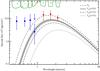 |
Fig. 6 Dayside flux measurements of WASP-46b compared with blackbody spectral energy distributions. Our measurements are shown as blue squares for the optical bands and as red circles for the NIR bands. The blue arrow shows the 3σ upper limit in the z′ band. Blackbody profiles of four temperatures are shown, including the JHK-weighted brightness temperature TB and three typical equilibrium temperatures (i.e., with f = 1/4,1/2,2/3, corresponding to planet-wide, dayside, no heat redistribution, respectively). The shaded area shows the uncertainties of the equilibrium temperature. |
In Fig. 6, we construct an SED for the thermal emission of WASP-46b based on our eclipse-depth measurements, and we show the corresponding flux-ratio spectrum in Fig. 7. The NIR measurements can be explained by an isothermal temperature profile of 2386 K, which is the weighted mean of the three brightness temperatures. The J, H, and K bands probe deep into the lower layers of the atmosphere because of weaker molecular absorptions at these bands. The isothermal temperature profile is expected to be present at the optical depth τ ~ 1 (Hansen 2008; Madhusudhan & Seager 2009; Guillot 2010).
Given the high temperature down in the atmosphere, if there is no internal energy source, it is unlikely that a strong thermal inversion exists in the upper atmosphere, otherwise the energy balance would be violated. The sign of temperature decreasing towards higher layer can tentatively be seen in the J, H, and K bands. Although temperatures in the three bands agree well with each other within the 1σ error bar and the best-fit temperatures of the J and H bands are almost the same, the best-fit K-band temperature is ~150 K lower. According to the NIR opacity curve (dominated by water), the J, H, and K bands probe the pressure layers that gradually increase (e.g., Barman 2008; Fortney et al. 2008). This indicates that the higher layer that is probed by the K band has a slightly lower temperature than the lower layer that is probed by the J and H bands.
On the other hand, the high equilibrium temperature (1654–2120 K, assuming AB = 0 and 1/4 ≤ f ≤ 2/3) possibly allows gaseous TiO and VO to be present in the upper atmosphere because Ti and V start to condense at 1670 K at 1 mbar (Fortney et al. 2008). However, the potential upper-atmosphere absorbers, such as the TiO and VO compounds or the sulfur compounds (Zahnle et al. 2009) or some unknown stratospheric absorbers, might have been destroyed by the high UV flux of the host star if the hypothesis proposed by Knutson et al. (2010) applies. The discovery paper (Anderson et al. 2012) has found a 16-day rotational modulation and weak Ca ii H+K for the host star. A recent study led by Shkolnik (2013) furthermore derived a high far-UV fractional luminosity log (LFUV/Lbol) = −4.546 ± 0.079 based on the NASA Galaxy Evolution Explorer (GALEX) measurements. The possible absence of high-altitude absorbers would indicate that there is no strong thermal inversion.
As a next step, more repeated NIR observations are needed to improve the confidence level of the measured eclipse depth, allowing us to accurately derive the heat redistribution efficiency. Furthermore, future measurements at longer wavelength, for example, warm Spitzer 3.6 μm and 4.5 μm, are crucial to construct the pressure-temperature profile and to decompose the molecular contents.
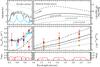 |
Fig. 7 Dayside planet-to-star flux ratios of WASP-46b compared with theoretical models. The optical and NIR are divided into left and right panels for better display scale. The top panels show the assumed theoretical models. Rayleigh scattering and atomic/molecular absorption profiles are assumed for the reflected light, where a Na/K model (blue) and a TiO/VO model (gray) from Fortney et al. (2008, 2010) are adopted for the absorption profiles. Blackbody profiles are assumed for the thermal emission light. The middle panels show the corresponding planet-to-star flux ratios. Our data points are shown in red circles with error bars, while the values that are integrated in each bandpass are shown in yellow (blue or gray for the optical) shapes. The bottom panels show the transmission curve of each band. |
4.3. Reflected light from the dayside atmosphere of WASP-46b?
Presuming that the tentative eclipse detections in the optical bands are real planetary signals instead of systematic false positives, we investigated what atmosphere they could deliver. As shown in Fig. 6, the optical measurements start to deviate from the blackbody emission profile blueward of the z′ band. The non-detection of the z′-band eclipse dip indicates that the emission at this band could be very low, while its 3σ upper limit in principal allows the 2386 K isothermal temperature profile. In contrast, the best-fit values of the g′-, r′-, i′-band measurements are clearly off the blackbody profile.
We derived the effective geometric albedos as listed in Table 2. The geometric albedo is defined as Ag = (Fp/F⋆)/(Rp/a)2. Assuming a blackbody emission of 2386 K, we corrected the thermal emission portion in the optical geometric albedos and list them in Table 2 as well. The values of these corrected geometric albedos appear to be very high. However, their large uncertainties degrade the significance, thus allowing the actual geometric albedos to be possibly lower. The quality of our measurements does not seem to warrant a detailed modeling of the optical spectrum. In Fig. 7, disregarding our NIR measurements, we construct two optical toy spectra composed of both reflection and emission for illustration purpose. The reflection portion was generated following the approach described by Evans et al. (2013), in which a Rayleigh scattering profile and two absorption profiles of the Fortney et al. (2008, 2010) models were combined to simulate the reflected light. Under the current simple assumption, the reflected light could account for the high flux ratios in the optical bands, indicating a high-altitude reflective cloud. However, since our NIR high brightness temperatures already suggest a very low Bond albedo, the high geometric albedos derived here are probably not real, unless the actual NIR eclipse depths are far shallower than the values measured here. Future transit spectroscopic observations in the optical as well as higher-precision NIR secondary-eclipse observations will be very useful to resolve this problem.
5. Conclusions
We observed one secondary eclipse of WASP-46b simultaneously in the g′r′i′z′JHK bands. We detected or tentatively detected the thermal emission in the J, H, K bands with a flux ratio of 0.129 ± 0.055%, 0.194 ± 0.078%, 0.253%, respectively. Corresponding brightness temperatures of 2453 K, 2462 K, 2306 K are consistent with an isothermal temperature profile of 2386 K. The slightly lower K-band temperature might indicate a decreasing temperature profile towards higher atmospheric layer. While the best-fit NIR brightness temperatures are all higher than the expected highest equilibrium temperature assuming zero albedo and no heat redistribution, they are still nearly consistent with the expected highest temperature at 1σ level, given their large uncertainties. Furthermore, we derived eclipse depths for the four optical bands. After correcting for the thermal emission portion, the geometric albedos still appear to be high, which is inconsistent with the low Bond albedo inferred from the NIR measurements. Future higher-precision observations are required to confirm our detections.
Online material
Appendix A: Light-curve baseline model selection
Tables A.1 and A.2 list the baseline coefficients of the chosen models for the seven light curves. Table A.3 gives five of the top-ranked baseline function models based on their BICs. The models that are numbered with one are the best chosen ones.
Baseline coefficients of the chosen models for the g′r′i′z′ light curves.
Baseline coefficients of the chosen models for the JHK light curves.
Top-ranked light-curve baseline models.
The rejection criterion at t = −0.05 days is somewhat arbitrary. We tried to avoid including the data with higher sky levels. We also tried to keep part of pre-ingress data to constrain the light-curve decorrelation. The compromise was made at the adopted time criterion, before which the slope of the sky values is steeper.
Acknowledgments
We are grateful to the anonymous referee for the careful reading and helpful comments that improved the manuscript. We thank Luigi Mancini for providing advice to improve this manuscript. G.C. acknowledges Chinese Academy of Sciences and Max Planck Society for the support of the doctoral training program. H.W. acknowledges the support by NSFC grants 11173060, 11127903, and 11233007. This work is supported by the Strategic Priority Research Program “The Emergence of Cosmological Structures” of the Chinese Academy of Sciences, Grant No. XDB09000000. Part of the funding for GROND (both hardware 84 and personnel) was generously granted by the Leibniz-Prize to G. Hasinger 85 (DFG grant HA 1850/28-1).
References
- Anderson, D. R., Collier Cameron, A., Gillon, M., et al. 2012, MNRAS, 422, 1988 [NASA ADS] [CrossRef] [Google Scholar]
- Barman, T. S. 2008, ApJ, 676, L61 [NASA ADS] [CrossRef] [Google Scholar]
- Burrows, A., Budaj, J., & Hubeny, I. 2008, ApJ, 678, 1436 [NASA ADS] [CrossRef] [Google Scholar]
- Cáceres, C., Ivanov, V. D., Minniti, D., et al. 2011, A&A, 530, A5 [NASA ADS] [CrossRef] [EDP Sciences] [Google Scholar]
- Chen, G., van Boekel, R., Madhusudhan, N., et al. 2014a, A&A, 564, A6 [NASA ADS] [CrossRef] [EDP Sciences] [Google Scholar]
- Chen, G., van Boekel, R., Wang, H., et al. 2014b, A&A, 563, A40 [NASA ADS] [CrossRef] [EDP Sciences] [Google Scholar]
- Cowan, N. B., & Agol, E. 2011, ApJ, 729, 54 [NASA ADS] [CrossRef] [Google Scholar]
- Croll, B., Lafrenière, D., Albert, L., et al. 2011, AJ, 141, 30 [NASA ADS] [CrossRef] [Google Scholar]
- Crossfield, I. J. M., Barman, T., Hansen, B. M. S., Tanaka, I., & Kodama, T. 2012, ApJ, 760, 140 [NASA ADS] [CrossRef] [Google Scholar]
- de Mooij, E. J. W., de Kok, R. J., Nefs, S. V., & Snellen, I. A. G. 2011, A&A, 528, A49 [NASA ADS] [CrossRef] [EDP Sciences] [Google Scholar]
- de Mooij, E. J. W., Brogi, M., de Kok, R. J., et al. 2013, A&A, 550, A54 [NASA ADS] [CrossRef] [EDP Sciences] [Google Scholar]
- Deming, D., Fraine, J. D., Sada, P. V., et al. 2012, ApJ, 754, 106 [NASA ADS] [CrossRef] [Google Scholar]
- Eastman, J., Siverd, R., & Gaudi, B. S. 2010, PASP, 122, 935 [NASA ADS] [CrossRef] [Google Scholar]
- Evans, T. M., Pont, F., Sing, D. K., et al. 2013, ApJ, 772, L16 [NASA ADS] [CrossRef] [Google Scholar]
- Ford, E. B. 2005, AJ, 129, 1706 [Google Scholar]
- Ford, E. B. 2006, ApJ, 642, 505 [NASA ADS] [CrossRef] [Google Scholar]
- Fortney, J. J., Lodders, K., Marley, M. S., & Freedman, R. S. 2008, ApJ, 678, 1419 [NASA ADS] [CrossRef] [Google Scholar]
- Fortney, J. J., Shabram, M., Showman, A. P., et al. 2010, ApJ, 709, 1396 [NASA ADS] [CrossRef] [Google Scholar]
- Gillon, M., Triaud, A. H. M. J., Fortney, J. J., et al. 2012, A&A, 542, A4 [NASA ADS] [CrossRef] [EDP Sciences] [Google Scholar]
- Greiner, J., Bornemann, W., Clemens, C., et al. 2008, PASP, 120, 405 [NASA ADS] [CrossRef] [Google Scholar]
- Guillot, T. 2010, A&A, 520, A27 [NASA ADS] [CrossRef] [EDP Sciences] [Google Scholar]
- Hansen, B. M. S. 2008, ApJS, 179, 484 [NASA ADS] [CrossRef] [Google Scholar]
- Knutson, H. A., Howard, A. W., & Isaacson, H. 2010, ApJ, 720, 1569 [NASA ADS] [CrossRef] [Google Scholar]
- Kurucz, R. L. 1979, ApJS, 40, 1 [NASA ADS] [CrossRef] [Google Scholar]
- Lee, J.-M., Fletcher, L. N., & Irwin, P. G. J. 2012, MNRAS, 420, 170 [NASA ADS] [CrossRef] [Google Scholar]
- Line, M. R., Zhang, X., Vasisht, G., et al. 2012, ApJ, 749, 93 [NASA ADS] [CrossRef] [Google Scholar]
- Loeb, A. 2005, ApJ, 623, L45 [NASA ADS] [CrossRef] [Google Scholar]
- Madhusudhan, N., & Seager, S. 2009, ApJ, 707, 24 [NASA ADS] [CrossRef] [Google Scholar]
- Madhusudhan, N., & Seager, S. 2010, ApJ, 725, 261 [NASA ADS] [CrossRef] [Google Scholar]
- Madhusudhan, N., Knutson, H., Fortney, J., & Barman, T. 2014, Protostars and Planets VI (University of Arizona Press), eds. H. Beuther, R. Klessen, C. Dullemond, & Th. Henning, accepted [arXiv:1402.1169] [Google Scholar]
- Mandel, K., & Agol, E. 2002, ApJ, 580, L171 [NASA ADS] [CrossRef] [Google Scholar]
- O’Rourke, J. G., Knutson, H. A., Zhao, M., et al. 2014, ApJ, 781, 109 [NASA ADS] [CrossRef] [Google Scholar]
- Ragozzine, D., & Wolf, A. S. 2009, ApJ, 698, 1778 [NASA ADS] [CrossRef] [Google Scholar]
- Schwarz, G. 1978, Annals of Statistics, 6, 461 [Google Scholar]
- Seager, S., & Deming, D. 2010, ARA&A, 48, 631 [NASA ADS] [CrossRef] [Google Scholar]
- Shkolnik, E. L. 2013, ApJ, 766, 9 [NASA ADS] [CrossRef] [Google Scholar]
- Wang, W., van Boekel, R., Madhusudhan, N., et al. 2013, ApJ, 770, 70 [NASA ADS] [CrossRef] [Google Scholar]
- Winn, J. N., Holman, M. J., Torres, G., et al. 2008, ApJ, 683, 1076 [NASA ADS] [CrossRef] [Google Scholar]
- Zahnle, K., Marley, M. S., Freedman, R. S., Lodders, K., & Fortney, J. J. 2009, ApJ, 701, L20 [NASA ADS] [CrossRef] [Google Scholar]
- Zhao, M., Milburn, J., Barman, T., et al. 2012a, ApJ, 748, L8 [NASA ADS] [CrossRef] [Google Scholar]
- Zhao, M., Monnier, J. D., Swain, M. R., Barman, T., & Hinkley, S. 2012b, ApJ, 744, 122 [NASA ADS] [CrossRef] [Google Scholar]
All Tables
All Figures
|
Fig. 1 Normalized sky level versus elapsed time. Blue, green, and red curves show the sky levels of the J, H, and K bands. For each band, all the values are normalized by its median, so as to illustrate the overall variation. Data that were acquired before the time indicated by the vertical dashed line are not included in our final analysis. Two dotted lines indicate the expected first and last contacts of the secondary eclipse based on the assumption of a circular orbit. |
| In the text | |
|
Fig. 2 Secondary-eclipse light curves of WASP-46b as observed with GROND in the g′r′i′z′ bands. Left panel: light curves that are normalized by the reference stars. Middle panel: baseline-corrected light curves that are binned every 10 min for display purpose. Right panel: best-fit light-curve residuals that are binned every 10 min. All the best-fit models are indicated by solid lines. |
| In the text | |
|
Fig. 3 Secondary-eclipse light curves of WASP-46b as observed with GROND in the JHK bands. Left panel: light curves that are normalized by the reference stars. Middle panel: baseline-corrected light curves that are binned every 10 min for display purpose. Right panel: best-fit light-curve residuals that are binned every 10 min. All the best-fit models are indicated by solid lines. |
| In the text | |
|
Fig. 4 Dependence of the measured flux ratio on the measured mid-eclipse time (converted to orbital phase) for the J (left), H (middle), and K (right) bands. Three contour levels correspond to the 1σ, 2σ, and 3σ confidence levels, respectively. |
| In the text | |
|
Fig. 5 Standard deviation of the best-fit light-curve residuals binned in different time resolutions. The vertical dashed line refers to the ingress/egress duration. The dashed red line presents the expected Poisson-like noise. The deviation above the dashed red line indicates time-correlated red noise. |
| In the text | |
|
Fig. 6 Dayside flux measurements of WASP-46b compared with blackbody spectral energy distributions. Our measurements are shown as blue squares for the optical bands and as red circles for the NIR bands. The blue arrow shows the 3σ upper limit in the z′ band. Blackbody profiles of four temperatures are shown, including the JHK-weighted brightness temperature TB and three typical equilibrium temperatures (i.e., with f = 1/4,1/2,2/3, corresponding to planet-wide, dayside, no heat redistribution, respectively). The shaded area shows the uncertainties of the equilibrium temperature. |
| In the text | |
|
Fig. 7 Dayside planet-to-star flux ratios of WASP-46b compared with theoretical models. The optical and NIR are divided into left and right panels for better display scale. The top panels show the assumed theoretical models. Rayleigh scattering and atomic/molecular absorption profiles are assumed for the reflected light, where a Na/K model (blue) and a TiO/VO model (gray) from Fortney et al. (2008, 2010) are adopted for the absorption profiles. Blackbody profiles are assumed for the thermal emission light. The middle panels show the corresponding planet-to-star flux ratios. Our data points are shown in red circles with error bars, while the values that are integrated in each bandpass are shown in yellow (blue or gray for the optical) shapes. The bottom panels show the transmission curve of each band. |
| In the text | |
Current usage metrics show cumulative count of Article Views (full-text article views including HTML views, PDF and ePub downloads, according to the available data) and Abstracts Views on Vision4Press platform.
Data correspond to usage on the plateform after 2015. The current usage metrics is available 48-96 hours after online publication and is updated daily on week days.
Initial download of the metrics may take a while.