| Issue |
A&A
Volume 567, July 2014
|
|
|---|---|---|
| Article Number | A11 | |
| Number of page(s) | 9 | |
| Section | The Sun | |
| DOI | https://doi.org/10.1051/0004-6361/201423698 | |
| Published online | 04 July 2014 | |
Blobs in recurring extreme-ultraviolet jets⋆
Key Laboratory for Dark Matter and Space Science, Purple Mountain Observatory, CAS, 210008 Nanjing, PR China
e-mail: zhangqm@pmo.ac.cn
Received: 23 February 2014
Accepted: 20 May 2014
Context. Coronal jets are one type of ubiquitous small-scale activity that is caused by magnetic reconnection in the solar corona. They are often associated with cool surges in the chromosphere.
Aims. In this paper, we report our discovery of blobs in the recurrent and homologous jets that occurred at the western edge of the NOAA active region 11259 on 2011 July 22.
Methods. The jets were observed in the seven extreme-ultraviolet (EUV) filters of the Atmospheric Imaging Assembly instrument aboard the Solar Dynamics Observatory. Using the base-difference images of the six filters (94, 131, 171, 211, 193, and 335 Å), we carried out the differential emission measure (DEM) analyses to explore the thermodynamic evolutions of the jets. The jets were accompanied by cool surges observed in the Hα line center of the ground-based telescope in the Big Bear Solar Observatory.
Results. The jets that had lifetimes of 20−30 min recurred at the same place for three times with an interval of 40−45 min. Interestingly, each of the jets intermittently experienced several upward eruptions at the speed of 120−450 km s-1. After reaching the maximum heights, they returned back to the solar surface, showing near-parabolic trajectories. The falling phases were more evident in the low-T filters than in the high-T filters, indicating that the jets experienced cooling after the onset of eruptions. We identified bright and compact blobs in the jets during their rising phases. The simultaneous presence of blobs in all the EUV filters were consistent with the broad ranges of the DEM profiles of the blobs (5.5 ≤ log T ≤ 7.5), indicating their multi-thermal nature. The median temperatures of the blobs were ~2.3 MK. The blobs that were ~3 Mm in diameter had lifetimes of 24−60 s.
Conclusions. To our knowledge, this is the first report of blobs in coronal jets. We propose that these blobs are plasmoids created by the magnetic reconnection as a result of tearing-mode instability and are ejected out along the jets.
Key words: Sun: chromosphere / Sun: corona / Sun: activity
Movies 1–3 associated to Figs. 1, 3, and 5 are available in electronic form at http://www.aanda.org
© ESO, 2014
1. Introduction
Coronal jets are transitory X-ray or extreme-ultraviolet (EUV) enhancements with an apparent collimated motion (Shibata et al. 1992). They were first observed by the Soft X-ray Telescope (SXT) aboard Yohkoh (Tsuneta et al. 1991). More and more coronal jets were observed by space-borne telescopes with higher resolutions and time cadences in the last two decades (Chae et al. 1999; Savcheva et al. 2007; Chifor et al. 2008; Nisticò et al. 2009; Shen et al. 2012; Moschou et al. 2012; Lee et al. 2013; Jiang et al. 2013). It is widely accepted that coronal jets are heated by magnetic reconnection between emerging flux and the pre-existing magnetic fields with opposite polarity (Shibata & Uchida 1986; Yokoyama & Shibata 1996; Moreno-Insertis et al. 2008; Török et al. 2009; Moreno-Insertis & Galsgaard 2013). According to the numerical simulations of Yokoyama & Shibata (1996), there are hot, compact microflares at their footpoints (Krucker et al. 2011; Zhang & Ji 2013) and cool Hα surges adjacent to the hot jets (Schmieder et al. 1995; Canfield et al. 1996; Liu & Kurokawa 2004; Jiang et al. 2007; Liu 2008; Nelson & Doyle 2013). The EUV emissions from a hot jet were observed to be absorbed by the foreground cool surge, which resulted in EUV dimming behind the leading edge of the jet (Zhang & Ji 2014). Pariat et al. (2009) proposed a new mechanism for the coronal hole jets as a result of continuous pumping of magnetic free energy and helicity into the upper solar atmosphere. The presence of dome-like magnetic topology that consists of a null point, a spine, and a separatrix surface in a X-ray bright point that was associated with recurrent jets was observed and reported by Zhang et al. (2012). Coronal jets are usually generated in coronal holes (Cirtain et al. 2007; Culhane 2007; Patsourakos et al. 2008; Chandrashekhar et al. 2014a) or at the edge of active regions (Kim et al. 2007; Guo et al. 2013; Schmieder 2013; Zhang & Ji 2014). The apparent heights and widths of jets are 10−400 Mm and 5−100 Mm. The velocities of jets are 10−1000 km s-1, which are on the same order of magnitude as the coronal Alfvén speed (Shimojo et al. 1996).
Recurrent jets and surges have often been observed and extensively been studied thanks to the everlasting development and improvement of the solar telescopes. Chae et al. (1999) analyzed simultaneous EUV data and Hα data from BBSO. Several EUV jets repeatedly occurred in the active region where pre-existing magnetic flux was canceled by newly emerging flux of opposite polarity. Chifor et al. (2008) analyzed a recurring solar active region jet that is observed in X-ray and EUV, finding a correlation between recurring magnetic cancellation and the X-ray jet emission. The jet emission was attributed to chromospheric evaporation flows due to recurring magnetic reconnection. Recurrent jets can also be caused by moving magnetic features (Brooks et al. 2007; Yang et al. 2013). Guo et al. (2013) reported the discovery of three EUV jets recurring in about one hour on 17 September 2010. According to the nonlinear force-free field extrapolation, the authors concluded that the magnetic reconnection occurred periodically in the current layer created between the emerging bipoles and the large-scale active region field, inducing the observed recurrent coronal jets. Murray et al. (2009) performed magnetohydrodynamic (MHD) numerical simulations of interaction between emerging flux and pre-existing magnetic fields in a coronal hole. When gas pressure of the reconnection outflow region exceeds that of the inflow region, the magnetic field lines in the two bounded outflow regions are driven to reconnect reversely, giving rise to an oscillatory reconnection and recurrent jets with the peak magnetic reconnection rate decreasing as time goes on. Pariat et al. (2010) performed 3D MHD simulations of periodic coronal jets due to a continuous twisting motion of the photosphere and pumping of magnetic free energy.
The temperatures of coronal jets have been extensively investigated since their discovery. There are mainly two methods for temperature diagnostics. One is filter-ratio assuming single temperature along the line-of-sight (LOS). It has been applied using the EUV 171 Å, 195 Å, and 284 Å filters or broadband soft X-ray filters (e.g., Shimojo & Shibata 2000; Nisticò et al. 2011; Madjarska 2011; Madjarska et al. 2012; Matsui et al. 2012; Pucci et al. 2013; Young & Muglach 2014). This approach, however, has its limitations and weaknesses. The reliable temperatures are limited within the monotonic range of the ratio of the temperature response functions of the two employed filters. The calculated temperature may represent the average temperature of the plasmas along the LOS. The other method is differential emission measure (DEM) based on the multi-thermal nature of the plasmas along the LOS (Doschek et al. 2010; Chandrashekhar 2014b; Kayshap et al. 2013; Chen et al. 2013; Sun et al. 2014b), which is more realistic and reasonable. Occasionally, hard X-ray (HXR) sources could be detected at the bottom of jets, and the hot thermal component could be isolated during the fittings to perform temperature diagnostic (Bain & Fletcher 2009; Krucker et al. 2011; Glesener et al. 2012). The temperatures of jets are 0.5−8 MK in the main body and even higher (10−30 MK) at the bottom, which have been reproduced in the multi-dimensional MHD numerical simulations (Nishizuka 2008; Archontis & Hood 2013).
Blob-like features or plasmoids are ubiquitous in the solar atmosphere. During the magnetic reconnections involved in solar flares, the electric current sheet may be subject to the tearing-mode instability (Furth et al. 1963), leading to the formation of multiple magnetic islands or plasmoids that are bidirectionally ejected out of the diffusion region (Ohyama & Shibata 1998; Kliem et al. 2000; Ko et al. 2003; Asai et al. 2004; Lin et al. 2005; Kołomański & Karlický 2007; Bárta et al. 2008; Nishizuka et al. 2010; Milligan et al. 2010; Takasao et al. 2012; Ni et al. 2012a,b; Kumar & Cho 2013). The plasmoid velocity is found to have a positive correlation with the reconnection rate (Nishida et al. 2009). White-light blobs are observed to be quasi-periodically ejected out of the large-scale coronal streamers (Song et al 2009). Recurrent plasmoids in the chromospheric anemone jets with a size of ~0.1 Mm are observed by Singh et al. (2012) and reproduced in the numerical simulations of Yang et al. (2013). In this paper, we investigated the thermodynamic evolutions of the recurrent and homologous jets observed by the Atmospheric Imaging Assembly (AIA; Lemen et al. 2012) aboard the Solar Dynamics Observatory (SDO) on 2011 July 22 and report our discovery of blobs in the jets. In Sect. 2, we describe the multi-wavelength data analysis followed by the results in Sect. 3. The discussion and the summary are presented in Sect. 4 and Sect. 5, respectively.
2. Data analysis
There are seven EUV filters (94, 131, 171, 193, 211, 304, and 335 Å) aboard the SDO/AIA instrument to achieve a wide temperature coverage (5.5 ≤ log T ≤ 7.5). On 2011 July 22, the homologous jets recurred for three times at the western edge of the NOAA active region (AR) 11259 during 21:00−23:30 UT. They were observed by AIA in all the EUV wavelengths with a time cadence of 12 s and resolution of 1 2. The level_1 fits data were calibrated using the standard program aia_prep.pro in the Solar Software. The images observed in different wavelengths were coaligned carefully using the cross-correlation method. Fortunately, the hot EUV jets were accompanied by cool Hα surges observed by the ground-based telescopes in the Big Bear Solar Observatory (BBSO) with a time cadence of 85−100 s and resolution of 2″. The Hα images were coaligned with the 304 Å images.
The observed intensity of an optically thin EUV line i is defined as 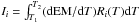 , where log T1 = 5.5 and log T2 = 7.5 stand for the minimum and maximum temperatures for the integral, Ri(T) denotes the temperature response function of line i, and
  represents the total column emission measure along the LOS. Here, ne stands for the electron number density. Therefore,
  means the differential emission measure. The DEM-weighted average temperature of the plasma along the LOS
  . A couple of methods and programs have been developed to reconstruct the DEM profiles using a set of EUV or SXR filters (e.g., Golub et al. 2004; Weber et al. 2004; 2005; Hannah & Kontar 2012; Aschwanden et al. 2013). Using six of the AIA filters (94, 131, 171, 211, 193, and 335 Å), Cheng et al. (2012) derived the DEM profiles and average temperatures of the three components of a coronal mass ejection (CME; Chen 2011) as observed by SDO: hot channel in the core region, the bright loop-like leading front, and coronal dimming in the wake of the CME (Cheng et al. 2013; Hannah & Kontar 2013). Recently, this method has also been applied to the temperature diagnostics of solar flares (Sun et al. 2014a) and failed filament eruption (Song et al. 2014). Since the jets were quite close to the active region, we selected the images before the onsets of the jets as base images and derived the base-difference images during the jets, so that the emissions and influences of the background corona were removed. We used the base difference images and the same method to reconstruct the DEM profiles and study the thermodynamic evolutions of the recurring jets. To evaluate the confidence in the reconstructed DEMs, we conducted Monte Carlo (MC) simulations, as described in detail in Cheng et al. (2012). The chi-square (χ2) of the 100 MC simulations is a measure of scatter of the DEM profiles. Lower values of χ2 mean smaller uncertainties in the DEM solution.
3. Results
3.1. Recurrent EUV jets
There were three recurrent and homologous EUV jets. The first jet (jet1) started at ~21:29 UT and reached the maximum height around 21:41 UT before falling back to the solar surface. Figure 1 shows jet1 observed at ~21:30:20 UT in six EUV filters. The jet was composed of a near-vertical collimated brightening that was 2.9 Mm in width at the top and a two-chamber structure at the bottom, which are commonplace in most inverse-Y-shaped coronal jets. However, a bright kernel visible in all the EUV wavelengths was ejected upwards along the jet as pointed by the white arrows.
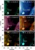 |
Fig. 1 Snapshots of jet1 seen in the six EUV filters at ~21:30:20 UT. The white arrows point to the blobs within the jet in panels a), b), c), e), and f). The white dashed line labeled with “cut1” in panel d) is used to investigate the longitudinal evolution of the jet whose time-slice diagram is displayed in Fig. 2. The temporal evolution of jet1 is shown in a movie (jet1.avi) available in the online edition. |
To study the longitudinal evolution of the jet, we extracted the intensity along the jet axis, which is labeled with “cut1” (75″ in length) and indicated by the white dashed line in Fig. 1d. The time-slice diagrams of cut1 in the seven EUV wavelengths are displayed in Fig. 2. It is revealed that jet1 underwent two main eruptions at the speed of ~435 km s-1 and ~136 km s-1 (Fig. 2d), which are followed by two weak and short eruptions that are more obvious in 171 Å (Fig. 2e) and 131 Å (Fig. 2f). The velocities of the two weak short eruptions were 271 km s-1 and 123 km s-1. The length of the jet reached maximum (35.6 Mm) at ~21:41 UT before decreasing to zero when the jet fell back to the solar surface at ~21:53 UT, which resulted in possible weak post-jet brightenings around 21:52 UT (see panels (e) and (f) in Fig. 2). The near-parabolic trajectory and the falling phase of the jet are more evident in the low-T filters (see panels (e), (f), and (g) in Fig. 2) than in the high-T filters (see panels (b), (c), and (d) in Fig. 2). Such a trajectory, similar to the case reported by Zhang & Ji (2014), indicates that the hot EUV jets underwent cooling owning to radiative loss and thermal conduction. The lifetime of jet1 is ~24 min.
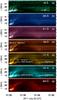 |
Fig. 2 Time-slice diagrams of cut1 in the seven filters during jet1. The white dotted lines in panel d) signify the two major eruptions of the jet with the slopes representing the rising speeds of 435 km s-1 and 136 km s-1, respectively. The major eruptions were followed by two weak and short eruptions illustrated by white dotted lines and pointed by the white arrows in panels e) and f). The slopes of the short dotted lines represent the velocities of the eruptions, being 271 km s-1 and 123 km s-1, respectively. The near-parabolic trajectory of the jet is more evident in the low-T filters (131, 171, and 304 Å) than in the high-T filters (211, 193, and 335 Å). Note the possible post-jet brightenings around 21:52 UT in panels e) and f). |
About a quarter after the end of jet1, the second collimated jet (jet2) occurred at the same place as the previous one. The bottom of the jet was composed of a couple of tiny bright kernels rather than a typical two-chamber structure. It started at ~22:10 UT and reached the maximum height at ~22:19 UT before falling back to the solar surface at ~22:34 UT. Figure 3 shows snapshots of the jet at ~22:11:20 UT in six of the EUV filters. Jet2, which was 5.4 Mm in width, was more inclined and diffused than jet1. There was also a compact and bright feature within jet2, which is pointed by the arrows.
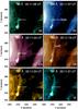 |
Fig. 3 Snapshots of jet2 seen in the six filters at ~22:11:20 UT. The white arrows point to the blobs within the jet in panels a), b), c), e), and f). The white dashed line labeled with “cut2” in panel d) is used to investigate the longitudinal evolution of the jet, whose time-slice diagram is displayed in Fig. 4. The temporal evolution of jet2 is shown in a movie (jet2.avi) available in the online edition. |
We extracted the intensity along the axis of jet2, which is labeled with “cut2” (71″ in length) and indicated by the white dashed line in Fig. 3d. The time-slice diagrams of cut2 in the seven filters are shown in Fig. 4. Starting at 22:07 UT, jet2 experienced a series of quasi-periodic eruptions with a period of ~65 s until 22:17 UT at the speed of ~311 km s-1, which are illustrated by the multiple white dashed dotted lines in Fig. 4e. Like jet1, jet2 also presented a near-parabolic trajectory, that is, plasma fell back to the solar surface after reaching the maximum height (31.7 Mm). The falling phase that ended at 22:35 UT was most distinct in the low-T wavelengths (see panels (e), (f), and (g)).
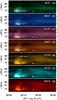 |
Fig. 4 Time-slice diagrams of cut2 in the seven filters during jet2. It experienced quasi-periodic upward eruptions with period of ~65 s during 22:07−22:17 UT at the speed of ~311 km s-1, which is indicated by the white dotted lines in panel e). |
After 22:52 UT, the third homologous jet (jet3) appeared but with a much shorter length and weaker intensity compared with the previous jets. Figure 5 shows snapshots of the jet in the six filters at ~22:55:35 UT. The bright and compact feature of jet3 is more evident in the 131, 171, and 335 Å images. We extracted the intensity along its axis, which is labeled with “cut3” (53″ in length) and indicated by the white dashed line in Fig. 5d. The time-slice diagrams of cut3 in the seven filters are displayed in Fig. 6. Like the previous jets, jet3 underwent intermittent eruptions, which are denoted by the white dotted lines in Fig. 6e, and reached maximum height (~11.2 Mm) before falling back to the solar surface. The rising velocities of the eruptions were ~311 km s-1. The near-parabolic trajectory of jet3 is clearly illustrated in the 131, 193, 171, and 304 Å images. The parameters of the three EUV jets are summarised in Table 1, including the maximum apparent heights, widths, apparent rising velocities, and lifetimes.
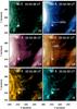 |
Fig. 5 Snapshots of jet3 seen in the six filters at ~22:55:35 UT. The white arrows point to the blobs within the jet in panels b), e), and f). The white dashed line labeled with “cut3” in panel d) is used to investigate the longitudinal evolution of the jet whose time-slice diagram is displayed in Fig. 6. The temporal evolution of jet3 is shown in a movie (jet3.avi) available in the online edition. |
Parameters of the three EUV jets.
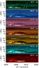 |
Fig. 6 Time-slice diagrams of cut3 in the seven filters during jet3. The white dotted lines in panel e) illustrate the intermittent eruptions of jet3 during 22:52−23:02 UT. The slopes of the dotted lines stand for the rising velocities of the eruptions, i.e., 311 km s-1. |
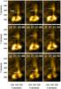 |
Fig. 7 a)−i) Nine snapshots of the AIA 171 Å images, showing the blobs during jet1, as pointed by the white arrows. |
3.2. Blobs in the jets
From the online movies that illustrate the evolutions of the recurrent jets, we identified more blobs. Figure 7 shows nine snapshots of the 171 Å images during jet1. The bright and compact kernels, as pointed by the white arrows, moved upwards from the bottom to the top of the jet during 21:30:12−21:31:12 UT and became blurred after mixing with the surroundings. After careful inspection, we found that the size of the blob increased slightly during the ejection. About 30 s later, another blob appeared at the bottom and rose until 21:32:12 UT. The sizes of the blobs were ~3 Mm. The intermittent appearances, upwards ejections, and disappearances of blobs were consistent with the sporadic eruptions of the jet, implying the bursty nature of magnetic reconnection in the jet.
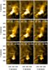 |
Fig. 8 a)−i) Nine snapshots of the AIA 171 Å images, showing the blobs during jet2, as pointed by the white arrows. |
Figure 8 displays nine snapshots of the 171 Å images during jet2 within which recurrent blobs were ejected. Despite of the high cadence of AIA (12 s), a blob was clearly present in 2−5 EUV snapshots due to their short lifetimes (24−60 s). Panels (d)−(f) illustrate the rising motion of a blob from the middle to top of the jet. Panels (h)−(i) show a blob that was restricted near the bottom of the jet.
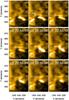 |
Fig. 9 (a)−(i) Nine snapshots of the AIA 171 Å images, showing the blobs during jet3, as pointed by the white arrows. |
Figure 9 displays nine snapshots of the 171 Å images during jet3. Compared with the previous two jets, the blobs were much fainter and reached lower heights. Panels (b)−(d) reveal that the blobs were close to the bottom of jet. Panels (e)−(i) illustrate the complete evolution of a blob. It appeared at 22:55:00 UT and reached maximum brightness at 22:55:12 UT before gradually mixing with the surroundings and fading out after 22:55:48 UT.
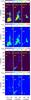 |
Fig. 10 Top two rows: EM a)−c) and temperature maps d)−f) of the jets during their rising phases. The arrows point to the blobs in the jets. The DEM curves of the plasmas in the boxes of a)−c) are displayed in Fig. 11. Bottom two rows: EM g)−i) and temperature maps j)−l) of the jets during their falling phases. Note that EM and Teff are in log -scales. |
We performed DEM analyses and derived the two-dimensional (2D) distributions of the EM and temperature (Teff) of the jets. Note that the minimum and maximum temperatures (T1 and T2) for the integral of EM are 105.5 K and 107.5 K. In Fig. 10, the top two rows demonstrate the selected EM and Teff maps of the jets during the rising phases of jet1 (left), jet2 (middle), and jet3 (right), respectively. The jets and blobs pointed by the yellow arrows are clearly present in the maps with higher emissions and temperatures than the adjacent quiet region. The two-chamber base of jet1 and the cusp-like bases of jet2 and jet3 with the highest emissions and temperatures are also clearly demonstrated in the maps. The bottom two rows demonstrate the selected EM and Teff maps of the jets during the falling phases of jet1 (left), jet2 (middle), and jet3 (right), respectively. It is seen that the emissions of the jets got quite weak and the temperatures decreased to a low level close to the adjacent quiet region, which is consistent with the time-slice diagrams of the jets in Figs. 2, 4, and 6.
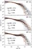 |
Fig. 11 The DEM profiles of the blob core regions of jet1 a), jet2 b), and jet3 c) indicated in the top panels of Fig. 10. The red solid lines stand for the best-fitted DEM curves from the observed values. The black dashed lines represent the reconstructed curves from the 100 MC simulations. The corresponding EM, Teff of the blobs, and the median values of χ2 of the MC simulations are displayed. |
In the top panels of Fig. 10, the core regions of blobs are included in the small yellow boxes with sizes of 1.8″. The base-difference EUV intensities within the boxes were averaged so that the core regions were taken as a whole. The DEM profiles of the first, second, and third blob cores are displayed in the top, middle, and bottom panels of Fig. 11, respectively. The red solid lines stand for the best-fitted profiles that are derived from the observed values, while the black dashed lines represent the profiles derived from the 100 MC simulations. It is obvious that the DEM profiles have a broad range between 5.5 ≤ log T ≤ 7.5, indicating that the blobs are multi-thermal in nature. However, the contributions of EM come mainly from the low-T plasma since the DEM decreases with log T. The reconstructions of the curves are most accurate and reliable in the range of 5.5 ≤ log T ≤ 6.5. The scatter increases with temperature in the range of 6.5 ≤ log T ≤ 7.5. The median values of the χ2 in the orders of 20 are labeled in Fig. 11. The Teff of the blob core regions of jet1, jet2, and jet3 are 2.2, 2.7, and 3.3 MK. The corresponding log EM are 27.5, 27.0, and 27.1, respectively. The average electron number densities of the blobs ne were estimated according to  (assuming filling factor ≈1), where EM and H stand for the EM and LOS depth of the blobs. Assuming that the jets are cylindric, the LOS depths equalled to the apparent widths of the blobs. The values of ne for the three blobs are 3.3, 1.9, and 2.1 × 109 cm-3, respectively. However, such estimations using the imaging data are very qualitative due to the large uncertainties of the plasma filling factor and the LOS column depth of the blobs. Considering the favorable perspectives of the Solar Terrestrial Relation Observatory (STEREO; Kaiser et al. 2005), we tried to find the counterparts of the jets in the EUV images observed by STEREO but failed due to the small scales and weak intensities of the jets. More precise diagnostics of the plasma densities should be conducted using the spectra-imaging observations.
We also derived the DEM curves of the blobs in jet1, jet2, and jet3 during their lifetimes. They are similar to those displayed in Fig. 11, featuring broad distributions and decreasing trends with temperature. Based on the DEM curves, we calculated the temperatures of the blobs in the three recurrent jets. The Teff ranges from 0.5 to 4 MK with an median value of 2.3 MK.
4. Discussion
4.1. Which type do the recurrent jet belong to?
Despite of their small scales, coronal jets usually present various morphology and characteristics. Nisticò et al. (2009) classified the 79 polar jets into four catalogues: Eiffel Tower-type jets, λ-type jets, micro-CME-type, and others. Based on the physical mechanisms, Moore et al. (2010) classified polar jets into standard and blowout jets. The former are the same as the well-known inverse-Y jets. The latter are counterparts of erupting-loop Hα macrospicules, where the jet-base magnetic arch undergoes a miniature version of the blowout eruptions that produce major CMEs. The main differences lie in whether the base arches have enough shear and twist to erupt open. Moore et al. (2013) carried out in-depth comparison and found that the blowout jets statistically have a cool component seen in 304 Å, lateral expansion, and axial rotation. The recurrent jets in our study matched the standard type, according to their morphology. However, they were present in all the EUV wavelengths of AIA, including the cool filters (304 Å). Lateral expansion and axial rotation, however, were absent in the jets. We have not noticed signatures of CME-like eruptions from the jet bases or curtain-like shapes after their eruptions as in the blowout jets. Therefore, we propose that the recurrent jets belong to the standard type though they had cool component.
4.2. Relationship between jets and surges
Coronal jets are always observed in the EUV and X-ray wavelengths, while surges are often observed in Hα due to their cool nature. According to the numerical simulations of Yokoyama & Shibata (1996), both hot (105−107 K) and cool (~104 K) plasma ejections are created side by side during the magnetic reconnection between the emerging flux and the pre-existing magnetic fields. The spatial relationship between the jets and surges is controversial. It has been observed that surges are adjacent to jets (Canfield et al. 1996; Chae et al. 1999; Jiang et al. 2007). In our study, the hot jets observed in the AIA filters were associated with recurrent cool surges that were observed and covered during their whole lifetimes in the Hα line center (Wang et al. 2014). In Fig. 12, we compared the 304 Å (left panels) and Hα (right panels) images that represent the three jets from top to bottom rows, respectively. We also superpose the intensity contours of the Hα images on the corresponding EUV images, finding that the surges were cospatial with the EUV dimmings behind the leading edges of the jets. After examining the movies of the recurrent jets in the other six EUV filters, we found that the dimmings visible in all the filters were cospatial with the surges. In the swirling flare-related jet on 2011 October 15 at the edge of AR 11314, Zhang & Ji (2014) discovered EUV dimming behind the leading edge of the jet, which was explained by the absorption of the EUV emissions of the hot jet by the foreground cool surge. Such explanation could be convincingly justified by our detailed and complete case study of recurrent jets. Considering that the jets and surges are 3D in nature (Moreno-Insertis & Galsgaard 2013), we believe that the differences of spatial relationship between the jet and surge lie in the different perspectives of observation. When the LOS is perpendicular to the plane determined by the jet and surge, they are adjacent to each other. However, when the LOS is parallel to the plane, they are cospatial and the EUV and X-ray emissions of the jets may be absorbed by the surges.
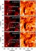 |
Fig. 12 Left panels: AIA 304 Å images during jet1 a), jet2 c), and jet3 e). The arrows point to the leading edges of the jets and the following dimming regions. Right panels: the near-simultaneous Hα images of the same FOV. The intensity contours of the Hα images are overlaid on the corresponding 304 Å images. |
4.3. Physical properties of the blobs
The magnetic islands or plasmoids associated with solar flares have extensively been observed and studied. Asai et al. (2004) discovered bursty sunward motions above the post-flare loops. The authors interpreted the bursty downflow as many plasmoids created inside the current sheet induced by the eruption of the large-scale filament. The velocities of the downflow were 45−500 km s-1, the electron number densities were 1−10×109 cm-3, and the sizes were 2−10 Mm. In our case, the rising velocities of the blobs in the jets were 120−450 km s-1, which were close to the values of the plasmoids associated with the big flare. The sizes (~3 Mm) of the blobs in the jets were also comparable to those of the flare-related plasmoids. Using the AIA multi-wavelength observations and the method of DEM reconstruction developed by Aschwanden et al. (2013), Kumar & Cho (2013) studied the bidirectional plasmoid ejections, whose DEM profiles have broad distributions, which are consistent with the cases of jet blobs in Fig. 11, implying the multi-thermal nature of the blobs. Based on the above comparison, we propose that the physical properties (temperature, velocity, and size) of the blobs that are intermittently ejected out of the recurring jets are quite close to those of the ejected plasmoids, which result from the tearing-mode instability of the current sheets where magnetic reconnections take place during big flares.
5. Summary
In this paper, we studied the recurrent and homologous jets that took place at the western edge of AR 11259 on 2011 July 22. The jets that had lifetimes of 20−30 min recurred three times with an interval of 40−45 min. Quasi-periodic eruptions were observed during each of the jets at the speed of 120−450 km s-1. After reaching the maximum heights, the jet plasmas returned back to the solar surface, showing near-parabolic trajectories. The falling phases were more evident in the low-T filters compared to that of the high-T filters, indicating that the jets experienced cooling due to radiative loss and thermal conduction after the onset of eruptions. We identified very bright and compact features, known here as blobs, in the jets during their rising phases. The simultaneous presences of blobs in all the EUV filters are consistent with the broad ranges of the DEM profiles of the blobs, indicating their multi-thermal nature. The DEM-weighted average temperatures of the blobs range from 0.5 to 4 MK with a median value of ~2.3 MK. The lifetimes of the blobs were 24−60 s. To our knowledge, this is the first report of blobs in coronal jets, and their physical properties are quite close to those of the bidirectionally ejected plasmoids during big flares, suggesting that the basic process of tearing-mode instability in current sheets exists not only in the large-scale solar flares but also in small-scale jets. Additional case studies and numerical simulations are required to get a better understanding of the blobs.
Online material
Movie of Fig. 1 Access here
Movie of Fig. 3 Access here
Movie of Fig. 5 Access here
Acknowledgments
The authors are grateful to the referee for the enlightening and valuable comments. Q.M.Z. acknowledges X. Cheng, T. H. Zhou, Y. N. Su, B. Kliem, L. Ni, P. F. Chen, M. D. Ding, C. Fang, R. Moore, E. Pariat, and the solar physics group in Purple Mountain Observatory for discussions and suggestions. SDO is a mission of NASA’s Living With a Star Program. AIA and HMI data are courtesy of the NASA/SDO science teams. The Hα data were obtained from the Global High Resolution Hα Network operated by the Big Bear Solar Observatory, New Jersey Institute of Technology. This work is supported by 973 program under grant 2011CB811402 and by NSFC 11303101, 11333009, 11173062 and 11221063.
References
- Archontis, V., & Hood, A. W. 2013, ApJ, 769, L21 [NASA ADS] [CrossRef] [Google Scholar]
- Asai, A., Yokoyama, T., Shimojo, M., & Shibata, K. 2004, ApJ, 605, L77 [NASA ADS] [CrossRef] [Google Scholar]
- Aschwanden, M. J., Boerner, P., Schrijver, C. J., & Malanushenko, A. 2013, Sol. Phys., 283, 5 [NASA ADS] [CrossRef] [Google Scholar]
- Bain, H. M., & Fletcher, L. 2009, A&A, 508, 1443 [NASA ADS] [CrossRef] [EDP Sciences] [Google Scholar]
- Bárta, M., Vršnak, B., & Karlický, M. 2008, A&A, 477, 649 [NASA ADS] [CrossRef] [EDP Sciences] [Google Scholar]
- Brooks, D. H., Kurokawa, H., & Berger, T. E. 2007, ApJ, 656, 1197 [NASA ADS] [CrossRef] [Google Scholar]
- Canfield, R. C., Reardon, K. P., Leka, K. D., et al. 1996, ApJ, 464, 1016 [NASA ADS] [CrossRef] [Google Scholar]
- Chae, J., Qiu, J., Wang, H., & Goode, P. R. 1999, ApJ, 513, L75 [NASA ADS] [CrossRef] [Google Scholar]
- Chandrashekhar, K., Bemporad, A., Banerjee, D., Gupta, G. R., & Teriaca, L. 2014a, A&A, 561, A104 [NASA ADS] [CrossRef] [EDP Sciences] [Google Scholar]
- Chandrashekhar, K., Morton, R. J., Banerjee, D., & Gupta, G. R. 2014b, A&A, 562, A98 [NASA ADS] [CrossRef] [EDP Sciences] [Google Scholar]
- Chen, N., Ip, W.-H., & Innes, D. 2013, ApJ, 769, 96 [NASA ADS] [CrossRef] [Google Scholar]
- Chen, P. F. 2011, Liv. Rev. Sol. Phys., 8, 1 [Google Scholar]
- Cheng, X., Zhang, J., Saar, S. H., & Ding, M. D. 2012, ApJ, 761, 62 [NASA ADS] [CrossRef] [Google Scholar]
- Cheng, X., Zhang, J., Ding, M. D., Liu, Y., & Poomvises, W. 2013, ApJ, 763, 43 [NASA ADS] [CrossRef] [Google Scholar]
- Chifor, C., Isobe, H., Mason, H. E., et al. 2008, A&A, 491, 279 [NASA ADS] [CrossRef] [EDP Sciences] [Google Scholar]
- Cirtain, J. W., Golub, L., Lundquist, L., et al. 2007, Science, 318, 1580 [NASA ADS] [CrossRef] [PubMed] [Google Scholar]
- Culhane, L., Harra, L. K., Baker, D., et al. 2007, PASJ, 59, 751 [Google Scholar]
- Doschek, G. A., Landi, E., Warren, H. P., & Harra, L. K. 2010, ApJ, 710, 1806 [NASA ADS] [CrossRef] [EDP Sciences] [Google Scholar]
- Furth, H. P., Killeen, J., & Rosenbluth, M. N. 1963, Phys. Fluids, 6, 459 [NASA ADS] [CrossRef] [Google Scholar]
- Glesener, L., Krucker, S., & Lin, R. P. 2012, ApJ, 754, 9 [NASA ADS] [CrossRef] [Google Scholar]
- Golub, L., Deluca, E. E., Sette, A., & Weber, M. 2004, The Solar-B Mission and the Forefront of Solar Physics, 325, 217 [NASA ADS] [Google Scholar]
- Guo, Y., Démoulin, P., Schmieder, B., et al. 2013, A&A, 555, A19 [NASA ADS] [CrossRef] [EDP Sciences] [Google Scholar]
- Hannah, I. G., & Kontar, E. P. 2012, A&A, 539, A146 [NASA ADS] [CrossRef] [EDP Sciences] [Google Scholar]
- Hannah, I. G., & Kontar, E. P. 2013, A&A, 553, A10 [NASA ADS] [CrossRef] [EDP Sciences] [Google Scholar]
- Jiang, Y. C., Chen, H. D., Li, K. J., Shen, Y. D., & Yang, L. H. 2007, A&A, 469, 331 [NASA ADS] [CrossRef] [EDP Sciences] [Google Scholar]
- Jiang, Y., Bi, Y., Yang, J., et al. 2013, ApJ, 775, 132 [NASA ADS] [CrossRef] [Google Scholar]
- Kaiser, M. L. 2005, Adv. Space Res., 36, 1483 [NASA ADS] [CrossRef] [Google Scholar]
- Kayshap, P., Srivastava, A. K., & Murawski, K. 2013, ApJ, 763, 24 [NASA ADS] [CrossRef] [Google Scholar]
- Kim, Y.-H., Moon, Y.-J., Park, Y.-D., et al. 2007, PASJ, 59, 763 [Google Scholar]
- Kliem, B., Karlický, M., & Benz, A. O. 2000, A&A, 360, 715 [NASA ADS] [Google Scholar]
- Ko, Y.-K., Raymond, J. C., Lin, J., et al. 2003, ApJ, 594, 1068 [NASA ADS] [CrossRef] [Google Scholar]
- Kołomański, S., & Karlický, M. 2007, A&A, 475, 685 [NASA ADS] [CrossRef] [EDP Sciences] [Google Scholar]
- Krucker, S., Kontar, E. P., Christe, S., Glesener, L., & Lin, R. P. 2011, ApJ, 742, 82 [NASA ADS] [CrossRef] [Google Scholar]
- Kumar, P., & Cho, K.-S. 2013, A&A, 557, A115 [NASA ADS] [CrossRef] [EDP Sciences] [Google Scholar]
- Lee, K.-S., Innes, D. E., Moon, Y.-J., et al. 2013, ApJ, 766, 1 [NASA ADS] [CrossRef] [Google Scholar]
- Lemen, J. R., Title, A. M., Akin, D. J., et al. 2012, Sol. Phys., 275, 17 [NASA ADS] [CrossRef] [Google Scholar]
- Lin, J., Ko, Y.-K., Sui, L., et al. 2005, ApJ, 622, 1251 [NASA ADS] [CrossRef] [Google Scholar]
- Liu, Y. 2008, Sol. Phys., 249, 75 [NASA ADS] [CrossRef] [Google Scholar]
- Liu, Y., & Kurokawa, H. 2004, ApJ, 610, 1136 [NASA ADS] [CrossRef] [Google Scholar]
- Madjarska, M. S. 2011, A&A, 526, A19 [NASA ADS] [CrossRef] [EDP Sciences] [Google Scholar]
- Madjarska, M. S., Huang, Z., Doyle, J. G., & Subramanian, S. 2012, A&A, 545, A67 [NASA ADS] [CrossRef] [EDP Sciences] [Google Scholar]
- Matsui, Y., Yokoyama, T., Kitagawa, N., & Imada, S. 2012, ApJ, 759, 15 [NASA ADS] [CrossRef] [Google Scholar]
- Milligan, R. O., McAteer, R. T. J., Dennis, B. R., & Young, C. A. 2010, ApJ, 713, 1292 [NASA ADS] [CrossRef] [Google Scholar]
- Moore, R. L., Cirtain, J. W., Sterling, A. C., & Falconer, D. A. 2010, ApJ, 720, 757 [NASA ADS] [CrossRef] [Google Scholar]
- Moore, R. L., Sterling, A. C., Falconer, D. A., & Robe, D. 2013, ApJ, 769, 134 [NASA ADS] [CrossRef] [Google Scholar]
- Moreno-Insertis, F., & Galsgaard, K. 2013, ApJ, 771, 20 [NASA ADS] [CrossRef] [Google Scholar]
- Moreno-Insertis, F., Galsgaard, K., & Ugarte-Urra, I. 2008, ApJ, 673, L211 [Google Scholar]
- Moschou, S. P., Tsinganos, K., Vourlidas, A., & Archontis, V. 2012, Sol. Phys., 310 [Google Scholar]
- Murray, M. J., van Driel-Gesztelyi, L., & Baker, D. 2009, A&A, 494, 329 [NASA ADS] [CrossRef] [EDP Sciences] [Google Scholar]
- Nelson, C. J., & Doyle, J. G. 2013, A&A, 560, A31 [NASA ADS] [CrossRef] [EDP Sciences] [Google Scholar]
- Ni, L., Roussev, I. I., Lin, J., & Ziegler, U. 2012a, ApJ, 758, 20 [NASA ADS] [CrossRef] [Google Scholar]
- Ni, L., Ziegler, U., Huang, Y.-M., Lin, J., & Mei, Z. 2012b, Phys. Plasmas, 19, 072902 [NASA ADS] [CrossRef] [Google Scholar]
- Nishida, K., Shimizu, M., Shiota, D., et al. 2009, ApJ, 690, 748 [NASA ADS] [CrossRef] [Google Scholar]
- Nishizuka, N., Shimizu, M., Nakamura, T., et al. 2008, ApJ, 683, L83 [NASA ADS] [CrossRef] [Google Scholar]
- Nishizuka, N., Takasaki, H., Asai, A., & Shibata, K. 2010, ApJ, 711, 1062 [NASA ADS] [CrossRef] [Google Scholar]
- Nisticò, G., Bothmer, V., Patsourakos, S., & Zimbardo, G. 2009, Sol. Phys., 259, 87 [NASA ADS] [CrossRef] [Google Scholar]
- Nisticò, G., Patsourakos, S., Bothmer, V., & Zimbardo, G. 2011, Adv. Space Res., 48, 1490 [NASA ADS] [CrossRef] [Google Scholar]
- Ohyama, M., & Shibata, K. 1998, ApJ, 499, 934 [NASA ADS] [CrossRef] [Google Scholar]
- Pariat, E., Antiochos, S. K., & DeVore, C. R. 2009, ApJ, 691, 61 [NASA ADS] [CrossRef] [Google Scholar]
- Pariat, E., Antiochos, S. K., & DeVore, C. R. 2010, ApJ, 714, 1762 [NASA ADS] [CrossRef] [Google Scholar]
- Patsourakos, S., Pariat, E., Vourlidas, A., Antiochos, S. K., & Wuelser, J. P. 2008, ApJ, 680, L73 [NASA ADS] [CrossRef] [Google Scholar]
- Pucci, S., Poletto, G., Sterling, A. C., & Romoli, M. 2013, ApJ, 776, 16 [NASA ADS] [CrossRef] [Google Scholar]
- Savcheva, A., Cirtain, J., Deluca, E. E., et al. 2007, PASJ, 59, 771 [NASA ADS] [Google Scholar]
- Schmieder, B., Shibata, K., van Driel-Gesztelyi, L., & Freeland, S. 1995, Sol. Phys., 156, 245 [NASA ADS] [CrossRef] [MathSciNet] [Google Scholar]
- Schmieder, B., Guo, Y., Moreno-Insertis, F., et al. 2013, A&A, 559, A1 [NASA ADS] [CrossRef] [EDP Sciences] [Google Scholar]
- Shen, Y., Liu, Y., Su, J., & Deng, Y. 2012, ApJ, 745, 164 [NASA ADS] [CrossRef] [Google Scholar]
- Shibata, K., & Uchida, Y. 1986, Sol. Phys., 103, 299 [NASA ADS] [CrossRef] [Google Scholar]
- Shibata, K., Ishido, Y., Acton, L. W., et al. 1992, PASJ, 44, L173 [NASA ADS] [CrossRef] [Google Scholar]
- Shimojo, M., & Shibata, K. 2000, ApJ, 542, 1100 [NASA ADS] [CrossRef] [Google Scholar]
- Shimojo, M., Hashimoto, S., Shibata, K., et al. 1996, PASJ, 48, 123 [NASA ADS] [CrossRef] [Google Scholar]
- Singh, K. A. P., Isobe, H., Nishizuka, N., Nishida, K., & Shibata, K. 2012, ApJ, 759, 33 [NASA ADS] [CrossRef] [Google Scholar]
- Song, H. Q., Chen, Y., Liu, K., Feng, S. W., & Xia, L. D. 2009, Sol. Phys., 258, 129 [NASA ADS] [CrossRef] [Google Scholar]
- Song, H. Q., Zhang, J., Cheng, X., et al. 2014, ApJ, 784, 48 [NASA ADS] [CrossRef] [Google Scholar]
- Sun, J. Q., Cheng, X., & Ding, M. D. 2014a, ApJ, 786, 73 [NASA ADS] [CrossRef] [Google Scholar]
- Sun, J. Q., Cheng, X., Guo, Y., Ding, M. D., & Li, Y. 2014b, ApJ, 787, L27 [NASA ADS] [CrossRef] [Google Scholar]
- Takasao, S., Asai, A., Isobe, H., & Shibata, K. 2012, ApJ, 745, L6 [NASA ADS] [CrossRef] [Google Scholar]
- Török, T., Aulanier, G., Schmieder, B., Reeves, K. K., & Golub, L. 2009, ApJ, 704, 485 [NASA ADS] [CrossRef] [Google Scholar]
- Tsuneta, S., Acton, L., Bruner, M., et al. 1991, Sol. Phys., 136, 37 [NASA ADS] [CrossRef] [Google Scholar]
- Wang, J.-f., Zhou, T.-h., & Ji, H.-s. 2014, Chin. Astron. Astrophys., 38, 65 [Google Scholar]
- Weber, M. A., Deluca, E. E., Golub, L., & Sette, A. L. 2004, Multi-Wavelength Investigations of Solar Activity, 223, 321 [NASA ADS] [Google Scholar]
- Weber, M. A., Schmelz, J. T., DeLuca, E. E., & Roames, J. K. 2005, ApJ, 635, L101 [NASA ADS] [CrossRef] [Google Scholar]
- Yang, L., He, J., Peter, H., et al. 2013, ApJ, 777, 16 [NASA ADS] [CrossRef] [Google Scholar]
- Yokoyama, T., & Shibata, K. 1996, PASJ, 48, 353 [NASA ADS] [CrossRef] [Google Scholar]
- Young, P. R., & Muglach, K. 2014, Sol. Phys., 24 [Google Scholar]
- Zhang, Q. M., & Ji, H. S. 2013, A&A, 557, L5 [NASA ADS] [CrossRef] [EDP Sciences] [Google Scholar]
- Zhang, Q. M., & Ji, H. S. 2014, A&A, 561, A134 [NASA ADS] [CrossRef] [EDP Sciences] [Google Scholar]
- Zhang, Q. M., Chen, P. F., Guo, Y., Fang, C., & Ding, M. D. 2012, ApJ, 746, 19 [NASA ADS] [CrossRef] [Google Scholar]
All Tables
All Figures
|
Fig. 1 Snapshots of jet1 seen in the six EUV filters at ~21:30:20 UT. The white arrows point to the blobs within the jet in panels a), b), c), e), and f). The white dashed line labeled with “cut1” in panel d) is used to investigate the longitudinal evolution of the jet whose time-slice diagram is displayed in Fig. 2. The temporal evolution of jet1 is shown in a movie (jet1.avi) available in the online edition. |
| In the text | |
|
Fig. 2 Time-slice diagrams of cut1 in the seven filters during jet1. The white dotted lines in panel d) signify the two major eruptions of the jet with the slopes representing the rising speeds of 435 km s-1 and 136 km s-1, respectively. The major eruptions were followed by two weak and short eruptions illustrated by white dotted lines and pointed by the white arrows in panels e) and f). The slopes of the short dotted lines represent the velocities of the eruptions, being 271 km s-1 and 123 km s-1, respectively. The near-parabolic trajectory of the jet is more evident in the low-T filters (131, 171, and 304 Å) than in the high-T filters (211, 193, and 335 Å). Note the possible post-jet brightenings around 21:52 UT in panels e) and f). |
| In the text | |
|
Fig. 3 Snapshots of jet2 seen in the six filters at ~22:11:20 UT. The white arrows point to the blobs within the jet in panels a), b), c), e), and f). The white dashed line labeled with “cut2” in panel d) is used to investigate the longitudinal evolution of the jet, whose time-slice diagram is displayed in Fig. 4. The temporal evolution of jet2 is shown in a movie (jet2.avi) available in the online edition. |
| In the text | |
|
Fig. 4 Time-slice diagrams of cut2 in the seven filters during jet2. It experienced quasi-periodic upward eruptions with period of ~65 s during 22:07−22:17 UT at the speed of ~311 km s-1, which is indicated by the white dotted lines in panel e). |
| In the text | |
|
Fig. 5 Snapshots of jet3 seen in the six filters at ~22:55:35 UT. The white arrows point to the blobs within the jet in panels b), e), and f). The white dashed line labeled with “cut3” in panel d) is used to investigate the longitudinal evolution of the jet whose time-slice diagram is displayed in Fig. 6. The temporal evolution of jet3 is shown in a movie (jet3.avi) available in the online edition. |
| In the text | |
|
Fig. 6 Time-slice diagrams of cut3 in the seven filters during jet3. The white dotted lines in panel e) illustrate the intermittent eruptions of jet3 during 22:52−23:02 UT. The slopes of the dotted lines stand for the rising velocities of the eruptions, i.e., 311 km s-1. |
| In the text | |
|
Fig. 7 a)−i) Nine snapshots of the AIA 171 Å images, showing the blobs during jet1, as pointed by the white arrows. |
| In the text | |
|
Fig. 8 a)−i) Nine snapshots of the AIA 171 Å images, showing the blobs during jet2, as pointed by the white arrows. |
| In the text | |
|
Fig. 9 (a)−(i) Nine snapshots of the AIA 171 Å images, showing the blobs during jet3, as pointed by the white arrows. |
| In the text | |
|
Fig. 10 Top two rows: EM a)−c) and temperature maps d)−f) of the jets during their rising phases. The arrows point to the blobs in the jets. The DEM curves of the plasmas in the boxes of a)−c) are displayed in Fig. 11. Bottom two rows: EM g)−i) and temperature maps j)−l) of the jets during their falling phases. Note that EM and Teff are in log -scales. |
| In the text | |
|
Fig. 11 The DEM profiles of the blob core regions of jet1 a), jet2 b), and jet3 c) indicated in the top panels of Fig. 10. The red solid lines stand for the best-fitted DEM curves from the observed values. The black dashed lines represent the reconstructed curves from the 100 MC simulations. The corresponding EM, Teff of the blobs, and the median values of χ2 of the MC simulations are displayed. |
| In the text | |
|
Fig. 12 Left panels: AIA 304 Å images during jet1 a), jet2 c), and jet3 e). The arrows point to the leading edges of the jets and the following dimming regions. Right panels: the near-simultaneous Hα images of the same FOV. The intensity contours of the Hα images are overlaid on the corresponding 304 Å images. |
| In the text | |
Current usage metrics show cumulative count of Article Views (full-text article views including HTML views, PDF and ePub downloads, according to the available data) and Abstracts Views on Vision4Press platform.
Data correspond to usage on the plateform after 2015. The current usage metrics is available 48-96 hours after online publication and is updated daily on week days.
Initial download of the metrics may take a while.