| Issue |
A&A
Volume 566, June 2014
|
|
|---|---|---|
| Article Number | A66 | |
| Number of page(s) | 18 | |
| Section | Stellar atmospheres | |
| DOI | https://doi.org/10.1051/0004-6361/201322697 | |
| Published online | 17 June 2014 | |
- Top
- Abstract
- 1. Introduction
- 2. Sample and data
- 3. The activity indices
- 4. Correlations between log
 and log IHα
 - 5. Mean activity level and correlations
- 6. Metallicity and correlations
- 7. Effective temperature and correlations
- 8. Discussion
- 9. Conclusions
- Online material
- Acknowledgments
- References
- List of tables
- List of figures
On the long-term correlation between the flux in the Ca ii H & K and Hα lines for FGK stars⋆
1 Centro de Astrofísica, Universidade do Porto, Rua das Estrelas, 4150-762 Porto, Portugal
e-mail: This email address is being protected from spambots. You need JavaScript enabled to view it.
2 Departamento de Física e Astronomia, Faculdade de Ciências, Universidade do Porto, 4169-007 Porto, Portugal
3 Observatoire de Genève, Université de Genève, 51 ch. des Maillettes, 1290 Versoix, Switzerland
Received: 17 September 2013
Accepted: 21 November 2013
Abstract
The re-emission in the cores of the Ca ii H & K and Hα lines are well known proxies of stellar activity. However, these activity indices probe different activity phenomena: the first is more sensitive to plage variation, while the other is more sensitive to filaments. In this paper, we study the long-term correlation between log R'HK and log IHα, two indices based on the Ca ii H & K and Hα lines, respectively, for a sample of 271 FGK stars using measurements obtained over a ~9 year time span. Because stellar activity is one of the main obstacles to the detection of low-mass and long-period planets, understanding this activity index correlation further can give us some hints about the optimal target to focus on ways to correct for these activity effects. We found a great variety of long-term correlations between log R'HK. Around 20% of our sample has a strong positive correlation between the indices while about 3% show strong negative correlation. These fractions are compatible with those found for the case of early-M dwarfs. Stars exhibiting a positive correlation have a tendency to be more active when compared to the median of the sample, while stars showing a negative correlation are more present among higher metallicity stars. There is also a tendency for the positively correlated stars to be more present among the coolest stars, a result which is probably due to the activity level effect on the correlation. Activity level and metallicity therefore seem to be playing a role on the correlation between log R'HK and log IHα. Possible explanations based on the influence of filaments for the diversity in the correlations between these indices are discussed in this paper. As a parallel result, we show a way to estimate the effective temperature of FGK dwarfs that exhibit a low activity level by using the Hα index.
Key words: stars: activity / stars: chromospheres / stars: solar-type / planetary systems
Appendices are available in electronic form at http://www.aanda.org
© ESO, 2014
1. Introduction
Stellar activity is one of the main limitations to the detection of low-mass and/or long-period planets using the radial-velocity method (e.g. Saar & Donahue 1997; Santos et al. 2000; Queloz et al. 2001; Boisse et al. 2009, 2011; Dumusque et al. 2011b; Lovis et al. 2011; Gomes da Silva et al. 2012). Fortunately, the radial-velocity noise induced by these effects can be corrected in some cases if for example the activity is simultaneously measured using activity indices (e.g. Dumusque et al. 2011a, 2012). Therefore, understanding the behaviour of activity indices and their relation with radial-velocity is vital to reduce the impact of activity in radial-velocity measurements and thus improve its sensitivity to planetary signals.
The re-emission in the Ca ii H & K lines are widely used proxies of activity-induced signals in radial-velocity measurements. However, the relation between this index and Hα is not well understood for solar-type stars. Since these two activity indices are affected by different activity phenomena in different ways (the emission in the centre of the Ca ii and Hα lines are not formed at the same temperature in the chromosphere), understanding their relationship and differences might bring new insights not only to stellar physics but also to the detection and characterisation of extrasolar planets.
It is known that there is a long-term correlation between the emission in the Ca ii H & K and Hα lines that follow the Sun’s 11-year activity cycle (Livingston et al. 2007). Other authors have suggested that the correlation is also present in other stars (Giampapa et al. 1989; Robinson et al. 1990; Strassmeier et al. 1990; Pasquini & Pallavicini 1991; Montes et al. 1995). However, when Cincunegui et al. (2007) measured simultaneously the flux in the two lines for a sample of 109 southern FGK and M stars, they found a large scatter in correlations, from very strong positive correlations to negative ones. They also suggested that the mean values of the flux in the Ca ii and Hα lines are correlated due to the effect of stellar colour on both fluxes.
Meunier & Delfosse (2009) studied the contribution of plages and filaments to the emission in Ca ii and Hα lines during a solar cycle. In their work, plages contribute to an increase in emission in both fluxes while filaments increase absorption in Hα only. They found that the contribution of filaments to Hα can be responsible for the decrease in the correlation coefficient between the two fluxes depending on their spatial distribution and contrast compared to those of plages. They also noted that the filament filling factor saturates at higher activity levels (e.g. cycle maxima) and the correlation between the two fluxes increases. Other factors contributing to a decrease in the measured correlation can be the time-span of observations, cycle phase at which they are measured, and stellar inclination angle. For example, the correlation is underestimated if the time-span is less than the cycle period (or the activity range is not well spanned).
Santos et al. (2010) studied the long-term activity of 8 FGK stars using the Ca ii H & K based SMW and Hα indices and found a general long-term correlation between the two. However, their sample was not large enough to have any statistical significance. Gomes da Silva et al. (2011) expanded the comparison between these two activity sensitive lines to early-M dwarfs. Similarly to Cincunegui et al. (2007) they detected a large variety of correlation coefficients, including anti-correlations for the least active stars in their sample. The most active stars were all, however, positively correlated. They also found hints that the Hα index was following an “anti-cycle” relative to their S-index in some cases, i.e., the maxima and minima measured in the two indices were anti-correlated. However, their time-span was not long enough to detect full cycles and confirm this effect.
In this paper, we analyse the behaviour of the flux in Ca ii H & K and Hα lines in FGK stars via two activity indices corrected for the effects of photospheric flux. We describe our sample and data in Sect. 2. The activity indices derivation, statistics, correlations between mean values, and activity cycle detectability are presented in Sect. 3 and Appendix A. The correlations between the two indices are discussed in Sect. 4. The distribution of the correlations in mean values of activity are discussed in Sect. 5. The effects of metallicity on the correlation are studied in Sect. 6, and the distribution of the correlations in effective temperature is presented in Sect. 7. We discuss possible causes for the existence of positive correlations and anti-correlations, and compare our results with those found for early-M dwarfs in Sect. 8. We conclude in Sect. 9. A possible use of the Hα index to estimate the effective temperature of low activity level FGK dwarfs is proposed in Appendix B.
2. Sample and data
The sample comes from ~400 FGK stars High Accuracy Radial Velocity Planet Searcher (HARPS, spectral resolution =115 000) high-precision sample that has been already used by Lovis et al. (2011) to study the long-term activity of FGK stars and its effect on the measurement of precise radial velocities. A description of the sample is presented in their paper. The spectra used in this work were obtained between February 2003 and February 2012. We used effective temperature, metallicity, and surface gravity that were already calculated for this sample by Sousa et al. (2008). Absolute magnitude and luminosity were both obtained from the Hipparcos catalogue.
We selected only spectra with S/N ≥ 100 at spectral order 56 (~5870 Å) and nightly averaged our measurements. Only stars with 10 or more nights of observations were selected. Then, we selected just the main sequence (MS) stars as in Lovis et al. (2011): we fitted a straight line through the H-R diagram and then excluded all stars with luminosity greater than +0.25 dex above that line.
We ended up with 271 MS stars with a median time span of ~7 years that we used for the rest of this work. This sample is comprised of 11 432 data points with a median of 23 nights of observations per star (and a maximum of 279). The sample ranges in spectral type from F8 to K6, effective temperature from 4595 to 6276 K, and metallicity from −0.84 to + 0.39 dex.
3. The activity indices
The  index, which is already corrected for the photospheric flux (Noyes et al. 1984), and respective errors were directly obtained from the HARPS DRS. This index is based on the S-index, which is calculated as the sum of the flux in two 0.6 Å bands centered at the calcium H (3968.47 Å) and K (3933.66 Å) lines divided by two 20 Å reference bands centered at 3900 and 4000 Å (see e.g. Boisse et al. 2009).
The Hα index and errors were calculated as in Gomes da Silva et al. (2011). We used a 1.6 Å band centered at 6562.808 Å and divided the flux in the central line by the flux in two reference bands of 10.75 and 8.75 Å that are centered at 6550.87 and 6580.31 Å, respectively. The flux errors were calculated as the photon noise in the line core,  , where N is the number of photons in the band. The activity indices errors were obtained via error propagation. The calibration of Hα for the effects of photospheric flux is presented in Appendix A and results in the IHα index.
3.1. Statistics of the log  index
index
Our sample, which is biased towards inactive stars to increase the chances of finding low-mass planets, has a median of −4.948 and a mean of −4.923. In this 271-star sample, only 22 (around 8%) are considered active stars with  , which lies on the higher activity region above the “Vaughan-Preston gap” (Vaughan & Preston 1980).
The star with the highest activity level is HD 224789 with  and the most inactive star is HD 181433 with
  . The median of the errors obtained for the index is 0.003, or in relative terms, 0.06% around the mean. In terms of variability, the median standard deviation of the sample is 0.0154 (0.3% around the mean) with HD 177758 being the least variable star with
  (0.07% around the mean) and HD 7199 being the star that varies the most with
  (1.6% around the mean).
3.2. Statistics of the log IHα index
In terms of log IHα, our sample has a median value of −1.7129 and a mean of −1.7118. The star with the highest log IHα mean value is HD 85119 with an activity level of −1.6562, and the most inactive star is HD 82516 with log IHα = −1.7299. The median of the errors we obtained for the log IHα index is 0.0002, or in relative terms, 0.01% around the mean. As stated before, we are only considering photon noise as a source of errors, and since the Hα line is in a brighter area of the spectrum compared to the Ca ii H & K lines, we expect the photon noise to be lower for IHα than for  . In terms of variability, the median standard deviation of the sample is 0.0019 (0.11% around the mean) with HD 74014 being the least variable star with σ(log IHα) = 0.0008 (0.05% around the mean) and HD 224789 being the star that varies the most with σ(log IHα) = 0.0063 (0.4% around the mean).
From these simple statistics, we can see that the is more sensitive to activity variations than log IHα. While has a median standard deviation of 0.3% of the mean, log IHα only has a median standard deviation of 0.1% of the mean, which means that has a more noticeable variation.
3.3. Mean activity level correlations
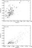 |
Fig. 1 Upper panel: relationship between |
Our activity indices are corrected for the effects of photospheric flux and can, if they are not dependent on other factors other than chromospheric flux, be used to compare the activity levels between different stars. Figure 1 (upper panel) shows the correlation between the mean values of and log IHα. These mean values were calculated by averaging the two indices over all our nightly measurements and represent the average activity level of each star. Open triangles are stars with a correlation coefficient of ρ ≥ 0.5, squares are stars with ρ ≤ − 0.5, and dots stars with no strong correlations. There is a correlation between the indices with a correlation coefficient of 0.53, but the scatter is large and the relation does not appear to be linear (cf. Cincunegui et al. 2007, Fig. 12). However, if we choose only the positively correlated stars (open triangles), they show a slightly more well defined relationship for the mean values with a correlation coefficient of 0.65. When Cincunegui et al. (2007) studied the correlation between the mean values of the flux in Ca ii and Hα, they concluded that the correlation between them is due to the dependence of the mean fluxes on stellar colour. Indeed, we have a stronger correlation with ρ = 0.79 when we plot the logarithm of the mean indices SMW vs. Hα (without colour correction) (Fig. 1, lower panel). We can therefore confirm that stellar colour is playing a role in the correlation between the mean flux levels of the Ca ii and Hα lines.
Variability and correlations using binned data for the stars with strong long-term correlations.
3.4. Activity cycles: detectability
To detect activity cycles, we fitted sinusoids to the time-series of the two activity indices. The significance of the fitting process was addressed by using an F-test, where  , to compare the fitting of a sinusoid with that of a constant model with σ being the standard deviation of the residuals of the fitted model. The probability p(F) gives the probability that the data is better fitted by a constant model than a sinusoidal function. We selected stars with cycles as the ones where probabilities, p(F)HK and p(F)Hα, are lower than 0.05 and, similarly to Lovis et al. (2011), we searched for periods in the region between 2 and 11 years.
Based on this selection criteria and using , we detected 69 stars (26%) with significant activity cycles with periods varying between 2.0 and 10.8 years. The log IHα index, however, is not so sensitive at detecting magnetic cycles. Only 9 stars (3.3%) showed significant cycles with periods varying between 3.9 and 9.5 years. As a comparison, Robertson et al. (2013) detected activity cycles with periods longer than one year in 5% of their sample of 93 K5-M5 stars using an Hα index similar to ours. In their study of activity cycles based on this sample but with a different selection criteria, Lovis et al. (2011) found that 99 stars (35%1) showed long-term activity cycles in their index, out of their 284-star sample. Their slightly higher fraction of stars with cycles is probably due to their use of a different selection criteria with a different restriction on the number of data points (some of their stars with detected cycles have less than 10 observations). We use only data with S/N ≥ 100, and we have more data points.
4. Correlations between log and log IHα
For all stars, we calculated the Pearson correlation coefficient between and log IHα. As was detected by Cincunegui et al. (2007) for the flux in the Ca ii H & K and Hα lines, we also find a great variety of correlation coefficients between and log IHα in the range −0.78 ≤ ρ ≤ 0.95 (Fig. 2). Although there is a tendency for the stronger correlations to be positive, we found a few cases of anti-correlations with ρ ≤ − 0.5.
Since we are interested in studying the cases of strong long-term correlations between the flux in the Ca ii H & K and Hα lines, we made a new selection of stars with good quality data that we are going to describe in the following section.
4.1. Stars with “strong” long-term correlations
We are interested in measuring the long-term Pearson correlation coefficient (ρ) between the and log IHα indices. Therefore, We need therefore to ensure that we have (a) a long time-span to certify that we are measuring long-term variations2, (b) variability in the long term so that we are not measuring correlations due to noise, (c) no short-term variations that can interfere with or hide the long-term ones, (d) enough quantity of points to calculate a significant ρ, and (e) strong correlations. To achieve this, we perform the following selection criteria on our 271-star sample:
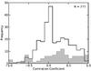 |
Fig. 2 Distribution of correlation coefficients between |
-
1.
All data was binned into 100-day averages. Each bin has at least three nights of observations, where the errors were calculated as the standard error on the mean, σ/
 , where σ is the standard deviation of the observations and N the number of observations. This reduces the variation induced by short-term activity modulated by stellar rotation.
 -
2.
We selected stars with at least four bins. This selection ensures that we have enough points to calculate ρ and that the time span is at least 400 days.
-
3.
Only stars that showed long-term variability in
were selected. This ensures that we are not detecting random variations due to noise. We performed an F-test on the binned data, where  , with σe the standard deviation of the binned data and ⟨ σi ⟩ the mean of the errors on the bins (e.g. Zechmeister et al. 2009). We calculated the probability of the F-test, P(F), such that the variations are due to the internal errors of the binned data, and selected stars with P(F) ≤ 0.05 (95% probability that the variability in not due to the internal errors).
 -
4.
We also applied the variability F-test for the log IHα index in a similar way as described above.
-
5.
To select significant correlation coefficients between
and log IHα, we calculated the False Alarm Probability (FAP) of having absolute values of ρ higher than the ones obtained for each star by bootstrapping the binned data and calculating the fraction of cases with higher | ρ | values. We used 10 000 permutations per star to calculate the FAP values. Only stars with FAP ≤ 0.05 (95% significance level) were selected. -
6.
Stars with strong correlations were selected as the ones having | ρ | ≥ 0.70.
From the 129 stars that passed selection criteria (1) and (2), 95 stars (73.6%) show long-term variability in , 51 stars (39.5%) show long-term variability in log IHα, and 45 stars (34.9%) show long-term variability on both indices. Out of the 45 stars that show variability on both indices, 12 stars (26.7%) show strong positive correlations between the indices, 10 of them (22.2%) have positive correlations, while two (4.4%) have anti-correlations.
Stellar parameters of the stars with strong long-term correlations.
Table 1 shows the variability and correlations data for the 12 stars with strong long-term correlations, where Nbins the number of bins for each star, ρ the correlation coefficient value, FAP the false alarm probability of ρ, and the parameters of the F-tests for both activity indices. The time series of , log IHα, and their respective correlations for these 12 stars are shown in Fig. B.1. We also tried to fit sinusoids to these stars (see Sect. 3.4) using the binned data of both indices to check if these stars have significant activity cycles. These fits appear in Fig. B.1 if the p(F)HK of the fit is lower than 0.05 (95% significance level). Two stars, HD 100508 and HD 78612, only have four bins and therefore do not have enough free parameters to calculate the probability of the fit. From the stars with more than four bins, three have p(F) values lower than 0.05 for the index, namely HD 4915, HD 63765, and HD 88742. These are all stars with strong positive correlations. The seven stars with significant cycles in have periods in the range 1528 to 10 665 days, and five of them could be fitted in log IHα with the same period found for and a p(F)Hα value lower than 0.05 (HD 13808, HD 154577, HD 215152, HD 7199, and HD 85512). For this sample, no star showed a period in log IHα that was not also found in and at a higher significance.
To try to understand why some stars have positive correlations while others are negative, we compared the correlations with the basic stellar parameters shown in Table 2. The two stars with negative correlations are shown in bold. First, we observe that the two stars with the negative correlations are two of the most inactive in terms of both and log IHα. Second, while all the stars with positive correlation coefficient have negative metallicity (median value of −0.20 dex), the two stars with negative correlations have positive metallicity (median value of 0.34 dex).
Although we can see hints that activity level and metallicity could be influencing the correlation between the two indices, the small number of stars we are using is insufficient to clearly show a solid trend between these parameters. We therefore chose to relax our selection criteria to increase the number of stars in our sample and check if the trends with activity level and metallicity are maintained.
4.2. “Relaxed” selection of stars with correlations
To increase the number of stars in our study, we discarded the variability tests, or FAPs on the correlation coefficients and used the full data sets based on the nightly averaged data. The correlation coefficient limit was also decreased to | ρ | ≥ 0.5. This produced a larger sample, which includes weaker correlations that can be due to a lower number of data points, shorter time-spans, and/or short-term variations. We shall therefore take this part of the study as an indication and not as a proof. However, we are now be able to do statistical tests to this sample.
Using this selection, we found that out of the 271 stars in our original sample, 58 (21.4% of the sample) have positive correlations between and log IHα, and 8 (3.0% of the sample) have anti-correlations. Table B.1 shows the 66 stars with | ρ | ≥ 0.5 with their activity mean levels and standard deviations, stellar parameters, and correlation coefficient between the two indices. Stars with correlations coefficients in the range −0.5 <ρ< 0.5 (no correlations) are presented in Table B.2.
All the eight stars with negative correlations (ρ ≤ − 0.5) have low activity levels with a median value of −4.97 and a median super-solar metallicity with a value of 0.20. The 58 stars with positive correlations (ρ ≥ 0.5) have with a median value of −4.81 and a median sub-solar metallicity with a value of −0.16. This “relaxed” selection appears to maintain the trends found in Sect. 4.1. In the next sections, we study these trends for this sample of stars.
5. Mean activity level and correlations
Here, we investigate the distribution of the positively and negatively correlated stars in terms of and log IHα activity levels.
Figure 3 (upper panel) shows the distribution of activity as measured by the index. The black line is the histogram of the selected sample of 271 main sequence stars. We can observe the selection bias against active stars as the great majority of the sample lies between −5.1 and −4.8 dex with a median of −4.95 dex. The hatched and filled grey histograms show the distribution in average activity level of the stars with positive and negative –log IHα correlations, respectively. The median of the negatively correlated stars is close to the median of the full sample (but with a tendency to be less active) with a value of −4.97 dex, while the median of the positively correlated stars lies in a higher activity zone with a value of −4.81 dex. In general, the majority of the least active stars show no strong correlations between the two indices. However, it is obvious from the plot that there is a tendency for the positively correlated stars to be more active in general, and all stars more active than  have positive correlations between and log IHα. The relative histogram in Fig. 3 (lower panel) illustrates very well this tendency.
The separation between positively and negatively correlated stars is further confirmed by the Kolmogorov-Smirnov (K-S) test that shows that the two populations are distinct with a p-value of 0.002 and a D value3 of 0.664. A similar distribution was found for log IHα (Fig. 4). The correlation between the two indices have different distributions according to activity level with negatively correlated stars being the least active ones and the positively correlated stars increasing in number with IHα activity level. In this case, the K-S test have a D = 0.513 and p-value = 0.03. The histograms also show that the values in log IHα are very well constrained between −1.73 and −1.70, and only a few cases of higher activity stars exists beyond these values. In the relative histogram (lower panel) note that the “hole” in the region between −1.675 and −1.660 is due to lack of data.
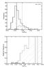 |
Fig. 3 Upper panel: distribution on |
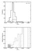 |
Fig. 4 Upper panel: distribution on log IHα activity for the full sample (black), stars with positive correlation coefficient higher than 0.5 (hatched grey), and stars with negative correlation coefficient lower than −0.5 (filled grey). Vertical lines are the medians of the distributions with a black line for the full sample, a dashed line for the positively correlated stars, and a dotted line for the negatively correlated stars. Lower panel: same as the upper panel but using a relative distribution on log IHα. |
6. Metallicity and correlations
Is stellar activity the only variable playing a role in the definition of the correlation or anti-correlation observed? In Table B.1, it is noticeable that there is a tendency for the eight stars with negative correlation between the and log IHα indices to have super-solar metallicity. We plotted the histogram of the two populations: the ones with a positive and those with a negative correlation against metallicity (Fig. 5). Symbols and colours are the same as that presented in Fig. 3. In Fig. 5 (upper panel), the median of the negatively correlated stars is not coincident with the medians of both the sample and the positively correlated stars. The histogram shows that, again, there seems to be two distinct populations of stars: the majority of the stars with positive correlations have negative metallicity while the negatively correlated stars appear to be of super-solar metallicity (mainly if compared to the overall sample). The sample median is −0.10 dex, and the median of positively correlated stars lies at −0.15 dex, but the negatively correlated star’s median is at a metallicity of 0.20 dex. This is further corroborated by the K-S test, which gives a probability of 0.04% that the two populations are indistinct (with a K-S D value of 0.733). The relative histogram of Fig. 5 (lower panel) confirms this with the negatively correlated stars peaking at the super-solar metallicity, while the positively correlated stars peaks at the sub-solar metallicity. Nevertheless, there are some stars with negative correlation that have sub-solar metallicity and stars with positive correlation with super-solar metallicity. We plotted metallicity histograms for two bins where there is superposition of positively and negatively correlated stars in activity in the region 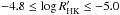 (Fig. 6). The tendency for stars with higher metal content to have negative correlations is maintained in each activity bin. In the lower panel of the figure for the three stars with metallicity between −0.1 and −0.2 dex, the positively correlated star has [Fe/H] = −0.20 dex, while the two negatively correlated stars have [Fe/H] = −0.16 and [Fe/H] = −0.15 dex. These plots show that metallicity still has an impact on the correlation between and log IHα for a given activity range.
Our analysis was based on a small number of anti-correlated stars, and our conclusions can be a consequence of small-number statistics. Also, as was stated before, this sample is not rigorous in terms of long-term variability of the stars or the significance of the correlations used. Further studies with a larger number of metal-rich stars would be crucial to confirm or refute these results.
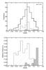 |
Fig. 5 Upper panel: distribution of metallicity for the full sample (black), stars with positive correlation coefficient higher than 0.5 (hatched grey), and stars with negative correlation coefficient lower than −0.5 (filled grey). The black vertical line is the median of the full sample, the dashed vertical line is the median of the positively correlated stars, and the dotted line is the median of the negatively correlated stars. Lower panel: same as the top panel but for relative distributions. The K-S test gives a p-value of 0.01% for the probability that the two populations are drawn from the same distribution. |
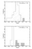 |
Fig. 6 Upper panel: distribution of metallicity for stars with positive correlation coefficient higher than 0.5 (hatched grey), and stars with negative correlation coefficient lower than −0.5 (filled grey) with activity in the range |
7. Effective temperature and correlations
We also analysed what would be the effect of temperature on the correlations between and log IHα. Figure 7 (upper panel) shows the distributions of the correlations for the full sample (black), the positively correlated stars (hatched grey), and negatively correlated stars (filled grey). There is an observational bias toward brighter stars and therefore hotter ones. However, the positively correlated stars seem very well distributed across the temperature range, which implies that there are more cooler stars having positive correlations than hotter stars relative to the full sample distribution. This can be easily observed in the lower panel of Fig. 7. Stars with negative correlations appear also well distributed in effective temperature but are only restricted to the range between ~5000 and ~6100 K. It would be easier then to find positively correlated stars among the cooler dwarfs. This effect is probably because cooler stars in our sample have a tendency to be more active than the hotter ones (Fig. 8). All the stars in our sample with  have effective temperatures lower than 5500 K. As we saw before in Sect. 5, all stars with activity higher than −4.7 have positive correlations.
Since the Mount Wilson survey, it is known that stellar age and mean activity level are related: younger stars exhibit higher activity levels than their older counterparts (Baliunas et al. 1995). Stars with 0.55 <B − V< 0.9, which are evolved, have lower activity levels than non-evolved stars (do Nascimento et al. 2003). Furthermore, Wright (2004) found that most of the stars classifieds as “flat” or “Maunder minimum”, which show very low activity and no variability, were evolved or sub-giant stars. Recently, Schröder et al. (2013) showed that the mean activity level decreases with relative MS-age. This confirms theorectical work by Reiners & Mohanty (2012). In other words, cooler K and M dwarfs did not had enough time to evolve (and decrease their activity level) so much as F-stars which evolve faster. We therefore observe cooler stars at a relative younger stage and, consequently, higher activity levels than their hotter counterparts.
The tendency for more earlier types in our sample is then a consequence of the bias towards fewer active stars due to the planetary search nature of this survey.
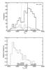 |
Fig. 7 Upper panel: distribution of effective temperature for the full sample (black), stars with positive correlation coefficient higher than 0.5 (hatched grey), and stars with negative correlation coefficient lower than −0.5 (filled grey). The black vertical line is the median of the full sample, the dashed vertical line is the median of the positively correlated stars, and the dotted line is the median of the negatively correlated stars. Lower panel: same as the top panel but for relative distributions. |
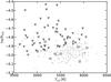 |
Fig. 8 Activity level measured by |
8. Discussion
8.1. Interpretation of the correlations via the effect of filaments and plages
So, why we sometimes see stars with anti-correlations (and “anti-cycles”) when we measure the flux in the Hα line? Meunier & Delfosse (2009) studied the contribution of plages and filaments to the SMW and Hα indices for the case of the Sun. They noted that the emission in the Ca ii lines increases in the presence of plages but is almost unaffected by filaments (their contribution is negligible). On the other hand, filaments contribute to the absorption in the flux of Hα, while plages contributes to emission. However, the filling factor of filaments saturates at a given activity level, while plages filling factor continues to increase as the activity level increases further. This saturation contributes to an increase in the correlation between the flux in the two line cores for higher activity levels. For the Sun, the filaments are not only found in active regions. They explain that, as the activity gets stronger (higher emission in the Ca ii lines), the positive correlation between the two indices is because the contribution of plages becomes more important for the Hα index than the contribution coming from filaments which saturates at a certain activity level. This produces the observed strong positive correlation between the two indices for higher activity stars as observed in Figs. 3 and 9. On the other hand, the low-activity stars with anti-correlation between the emission in Ca ii and Hα, which appear in Figs. 3 and 9, can be explained if these stars have the filaments with a strong contrast (compared to plages) and which have not reached their saturation limit (due to their low activity levels).
The occurrence of positively correlated stars at higher activity levels and negatively correlated stars at lower activity levels, which we observe in Sect. 5, can then be explained by the effect of filaments on the flux of the Hα line.
If the positively and negatively correlated stars are two different populations in terms of metallicity as discussed in Sect. 6 and if the ratio of the contrast/filing factor of filaments to plages is responsible for the anti-correlation between the flux in the Ca ii H & K and Hα lines, then metallicity might have an effect on the presence of filaments (or their contrast and/or filling factor) in the stellar corona. This could be used to predict the correlation between these two indices and to forecast the presence, contrast, and/or filling factor between plages and filaments for a given star.
8.2. Comparison with M dwarfs
In a previous work, Gomes da Silva et al. (2011) studied the long-term activity of 30 M0-M5 dwarfs and found hints of Hα “anti-cycles” (inverted in comparison to the cycles) on some stars of their sample. The potential maxima and minima of some stars were anti-correlated. This can be an indication that the physical mechanisms responsible for the anti-correlation, and thus “anti-cycles” between the two indices are present in both solar-type stars and at least in the earlier M dwarfs. The authors also found that all M-dwarfs in their sample have positive correlations after a certain value of S-index activity and found a case of an anti-correlation with a correlation coefficient value lower than −0.5 in the least active stars zone (see their Fig. 3). We should note, however, that their S-index was not corrected for the effects of photospheric flux, and therefore there is a temperature contribution to the mean index values that varies from star to star. Nevertheless, their distribution of correlations is compatible with ours in the sense that after a certain level of activity all active stars have positive correlations, and there are some cases of low activity stars with anti-correlations (Fig. 9). Since both FGK and early M stars have radiative cores with convective envelopes, their activity phenomena might not be too different (contrary to later M dwarfs which are fully convective). Therefore, if the contribution of filaments to the Hα absorption is the sole responsible to the anti-correlation between the flux in the Ca ii and Hα lines, then it is possible that this phenomenon is occurring in a similar way for the two types of stars.
Further studies of the correlations between the two indices for later M dwarfs would be interesting to understand how the behaviour of the two indices evolve in spectral type and infer about the presence of filaments in fully convective stars.
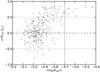 |
Fig. 9 Correlation coefficient of the relation between |
9. Conclusions
We studied the correlation between the flux in the Ca ii H & K and Hα lines via two activity indices, and IHα, corrected for photospheric flux. A sample of 271 low activity FGK stars observed during ~9 years was used to this effect. This study was the larger scale study (in both sample number and time-span) of the correlation between these two chromospheric indices for solar-type stars.
We detected significant activity cycles in 69 stars (26% of our sample) using the index but only in 9 stars (3.3%) using log IHα. The Hα line is not so sensitive at measuring long-term variations as the Ca ii lines. We also found a great variety of correlation coefficients in the range −0.78 ≤ ρ ≤ 0.95, similar to what was found by Cincunegui et al. (2007). Possible explanations for this variety are given by Meunier & Delfosse (2009) and include the spatial distribution and difference in contrast of filaments relative to plages.
To study the correlation between the and log IHα indices, we first selected only the stars showing “strong” long-term correlations between the two indices by applying a rigorous selection criteria based on variability F-tests, using FAPs on the correlation coefficients and binning the data to 100-day bins. This selection criteria returned a sample of 12 stars, where two of them have anti-correlations and the rest positive correlations. We observed that the two stars with anti-correlations have tendency to have lower activity levels and super-solar metallicity when compared to the positively correlated stars.
Since this rigorous selection returned a small number of stars, we relaxed the selection criteria to increase our sample and study the trends found with the rigorous selection. Using this selection criteria we found that:
-
58 stars (21% out of 271) have positive correlations (with ρ ≥ 0.5) and 8 stars (3% out of 271) show anti-correlations (with ρ ≤ − 0.5). These numbers are compatible with those found by Gomes da Silva et al. (2011) for early-M dwarfs. Some of the stars with strong anti-correlations show “anti-cycles” measured in log IHα: negative activity cycles when compared to those measured by
. -
The stars with positive correlation between the two indices have a tendency to be more active than those with negative correlations. All the stars with
 have positive correlation between the indices. We interpret this behaviour using the results from Meunier & Delfosse (2009) that the contribution to absorption in the Hα line by filaments saturates after a certain level of activity, and only plages contribute to emission in both Ca ii and Hα.
 -
We also found a tendency for the stars with negative correlations to be more metal rich than the rest of the sample and that this holds for stars of similar activity level.
-
The distribution of the correlations in effective temperature was also studied, and we detected that there are more cooler stars showing positive correlations than hotter stars in relative terms. This is because cooler stars in our sample are in general more active than hotter ones, and there is a tendency for the more active stars to have positive correlations.
-
As a parallel result, we found that our Hα index can be used to estimate the effective temperature of a low-activity FGK star.
These results might affect planet detections since activity is one of the main source of errors in radial velocity (and photometric) measurements. It would be interesting to compare the correlation between the flux in the Ca ii H & K and Hα lines with the measured radial velocity and see if this correlation has any effect on the observed radial velocity signal.
Online material
Appendix A: The IHα hydrogen line based activity index
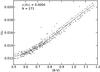 |
Fig. A.1 Calibration of Hα index as a function of (B − V) colour. The solid curve line is the best fit to the data and the dashed lines correspond to the 1–σ limits. |
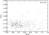 |
Fig. A.2 Dependence of the log IHα index on stellar colour. |
The Hα index is calculated from the fraction of the flux in the Hα line centre to the flux in two continuum reference bands, where one bluer other redder than the hydrogen line. This is sufficient if we are interested in determining the activity evolution over time for a star. However, stars with different colours have different amounts of flux in the continuum, and this makes the average Hα level not comparable between different stars due to a systematic error introduced by the photospheric flux interference in the measurements (e.g. Cincunegui et al. 2007).
To be able to compare the average Hα index between different stars, the photospheric contribution to the index needs to be taken into account. Figure A.1 shows the calibration of Hα to the effects of stellar colour. We fitted Hα to (B − V) using a cubic
polynomial, which resulted in a standard deviation of the fit of 0.0004. Our corrected IHα activity index is then  (A.1)Figure A.2 shows that the resulting index is not dependent on (B − V) and can therefore be used to compare the activity level of stars of different colour. This calibration is valid for main sequence stars with (B − V) colour between 0.5 and 1.2 and has mean Hα activity levels between 0.012 and 0.021.
Appendix B: Estimating effective temperature using the flux in Hα line
The Hα line wings are known to be a proxy of effective temperature (e.g. Fuhrmann et al. 1993; Barklem et al. 2002) and are sometimes used to confirm more accurate results by other methods. For example, Bouchy et al. (2008) used the wings of the Hα line to derive a temperature of 5450 ± 120 K for the star CoRoT-Exo-2. Sozzetti et al. (2007) compared the Hα wings to those of synthetic spectra to obtain a temperature region of 5750−6000 K for TrES-2 (other authors that used the same technique as a rogue estimate of temperature include Santos et al. 2006; Sozzetti et al. 2009).
We found that our Hα activity index is also a good proxy of Teff. Figure B.1 shows a quadratic fit to the correlation between these parameters. Active stars (open circles) were not used due to their contribution to a larger scatter. We obtained an rms of the Teff residuals of σ = 68 K, and a correlation coefficient of ρ = −0.96. The calibrated Teff is of the form  (B.1)This equation can be used for dwarfs with log IHK ≤ − 4.70, mean Hα activity in the range 0.012 ≤ Hα ≤ 0.021, and effective temperatures in the range 4600 ≤ Teff ≤ 6280 K.
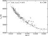 |
Fig. B.1 Calibration of Teff by using Hα activity index for all main sequence stars except the most active (log IHK ≥ − 4.75, open circles). The grey line is the best quadratic fit to the data. |
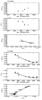 |
Fig. B.1 Time-series of |
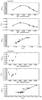 |
Fig. B.1 continued. |
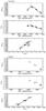 |
Fig. B.1 continued. |
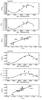 |
Fig. B.1 continued. |
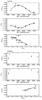 |
Fig. B.1 continued. |
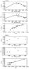 |
Fig. B.1 continued. |
Parameters for the 66 stars with | ρ | ≥ 0.5 from the nightly averaged 271-star sample.
Parameters for the 205 stars with |ρ| ≤ 0.5 from the nightly averaged 271-star sample.
We should note that they do not find cycles for 165 stars but they cannot exclude cycles either. In their conclusions, they arrive at a final value of 61% of stars with cycles when they exclude these stars from the fraction.
Since this sample derives from a planet hunt selection of stars, active stars with were monitored early and only rarely measured. Therefore, stars with higher activity have fewer measurements and possibly a lower time-span of observations. This selection thus reduces even more the number of active stars in the sample.
The K-S D value is the highest value of the difference between the cumulative distributions of the two populations. The p-value gives the probability that the two populations come from the same parent distribution.
Acknowledgments
This work has been supported by the European Research Council/European Community under the FP7 through a Starting Grant, as well as in the form of a grant reference PTDT/CTE-AST/098528/2008, funded by Fundação para a Ciência e a Tecnologia (FCT), Portugal. J.G.S. would like to thank the financial support given by FCT in the form of a scholarship, namely SFRH/BD/64722/2009. N.C.S. would further like to thank the support from FCT through a Ciência 2007 contract funded by FCT/MCTES (Portugal) and POPH/FSE (EC). I.B. also acknowledges the financial support given by FCT in the form of grant reference SFRH/BPD/81084/2011.
References
- Baliunas, S. L., Donahue, R. A., Soon, W. H., et al. 1995, ApJ, 438, 269 [NASA ADS] [CrossRef] [Google Scholar]
- Barklem, P. S., Stempels, H. C., Allen de Prieto, C., et al. 2002, A&A, 385, 951 [NASA ADS] [CrossRef] [EDP Sciences] [Google Scholar]
- Boisse, I., Moutou, C., Vidal-Madjar, A., et al. 2009, A&A, 495, 959 [NASA ADS] [CrossRef] [EDP Sciences] [Google Scholar]
- Boisse, I., Bouchy, F., Hébrard, G., et al. 2011, A&A, 528, A4 [NASA ADS] [CrossRef] [EDP Sciences] [Google Scholar]
- Bouchy, F., Queloz, D., Deleuil, M., et al. 2008, A&A, 482, L25 [NASA ADS] [CrossRef] [EDP Sciences] [Google Scholar]
- Cincunegui, C., Díaz, R. F., & Mauas, P. J. D. 2007, A&A, 469, 309 [NASA ADS] [CrossRef] [EDP Sciences] [Google Scholar]
- do Nascimento, Jr., J. D., Canto Martins, B. L., Melo, C. H. F., Porto de Mello, G., & De Medeiros, J. R. 2003, A&A, 405, 723 [NASA ADS] [CrossRef] [EDP Sciences] [Google Scholar]
- Dumusque, X., Lovis, C., Ségransan, D., et al. 2011a, A&A, 535, A55 [NASA ADS] [CrossRef] [EDP Sciences] [Google Scholar]
- Dumusque, X., Santos, N. C., Udry, S., Lovis, C., & Bonfils, X. 2011b, A&A, 527, A82 [NASA ADS] [CrossRef] [EDP Sciences] [Google Scholar]
- Dumusque, X., Pepe, F., Lovis, C., et al. 2012, Nature, 491, 207 [NASA ADS] [CrossRef] [PubMed] [Google Scholar]
- Fuhrmann, K., Axer, M., & Gehren, T. 1993, A&A, 271, 451 [NASA ADS] [Google Scholar]
- Giampapa, M. S., Cram, L. E., & Wild, W. J. 1989, ApJ, 345, 536 [NASA ADS] [CrossRef] [Google Scholar]
- Gomes da Silva, J., Santos, N. C., Bonfils, X., et al. 2011, A&A, 534, A30 [NASA ADS] [CrossRef] [EDP Sciences] [Google Scholar]
- Gomes da Silva, J., Santos, N. C., Bonfils, X., et al. 2012, A&A, 541, A9 [NASA ADS] [CrossRef] [EDP Sciences] [Google Scholar]
- Livingston, W., Wallace, L., White, O. R., & Giampapa, M. S. 2007, ApJ, 657, 1137 [NASA ADS] [CrossRef] [Google Scholar]
- Lovis, C., Dumusque, X., Santos, N. C., et al. 2011, A&A, submitted [arXiv:1107.5325] [Google Scholar]
- Meunier, N., & Delfosse, X. 2009, A&A, 501, 1103 [NASA ADS] [CrossRef] [EDP Sciences] [Google Scholar]
- Montes, D., Fernandez-Figueroa, M. J., de Castro, E., & Cornide, M. 1995, A&A, 294, 165 [NASA ADS] [Google Scholar]
- Noyes, R. W., Hartmann, L. W., Baliunas, S. L., Duncan, D. K., & Vaughan, A. H. 1984, ApJ, 279, 763 [NASA ADS] [CrossRef] [Google Scholar]
- Pasquini, L., & Pallavicini, R. 1991, A&A, 251, 199 [NASA ADS] [Google Scholar]
- Queloz, D., Henry, G. W., Sivan, J. P., et al. 2001, A&A, 379, 279 [NASA ADS] [CrossRef] [EDP Sciences] [Google Scholar]
- Reiners, A., & Mohanty, S. 2012, ApJ, 746, 43 [NASA ADS] [CrossRef] [Google Scholar]
- Robertson, P., Endl, M., Cochran, W. D., & Dodson-Robinson, S. E. 2013, ApJ, 764, 3 [NASA ADS] [CrossRef] [Google Scholar]
- Robinson, R. D., Cram, L. E., & Giampapa, M. S. 1990, ApJS, 74, 891 [NASA ADS] [CrossRef] [Google Scholar]
- Saar, S. H., & Donahue, R. A. 1997, ApJ, 485, 319 [NASA ADS] [CrossRef] [Google Scholar]
- Santos, N. C., Mayor, M., Naef, D., et al. 2000, A&A, 361, 265 [NASA ADS] [Google Scholar]
- Santos, N. C., Pont, F., Melo, C., et al. 2006, A&A, 450, 825 [NASA ADS] [CrossRef] [EDP Sciences] [Google Scholar]
- Santos, N. C., Gomes da Silva, J., Lovis, C., & Melo, C. 2010, A&A, 511, A54 [NASA ADS] [CrossRef] [EDP Sciences] [Google Scholar]
- Schröder, K.-P., Mittag, M., Hempelmann, A., González-Pérez, J. N., & Schmitt, J. H. M. M. 2013, A&A, 554, A50 [NASA ADS] [CrossRef] [EDP Sciences] [Google Scholar]
- Sousa, S. G., Santos, N. C., Mayor, M., et al. 2008, A&A, 487, 373 [NASA ADS] [CrossRef] [EDP Sciences] [MathSciNet] [Google Scholar]
- Sozzetti, A., Torres, G., Charbonneau, D., et al. 2007, ApJ, 664, 1190 [NASA ADS] [CrossRef] [Google Scholar]
- Sozzetti, A., Torres, G., Charbonneau, D., et al. 2009, ApJ, 691, 1145 [NASA ADS] [CrossRef] [Google Scholar]
- Strassmeier, K. G., Fekel, F. C., Bopp, B. W., Dempsey, R. C., & Henry, G. W. 1990, ApJS, 72, 191 [NASA ADS] [CrossRef] [Google Scholar]
- Vaughan, A. H., & Preston, G. W. 1980, PASP, 92, 385 [NASA ADS] [CrossRef] [Google Scholar]
- Wright, J. T. 2004, AJ, 128, 1273 [NASA ADS] [CrossRef] [Google Scholar]
- Zechmeister, M., Kürster, M., & Endl, M. 2009, A&A, 505, 859 [NASA ADS] [CrossRef] [EDP Sciences] [Google Scholar]
All Tables
Variability and correlations using binned data for the stars with strong long-term correlations.
Parameters for the 66 stars with | ρ | ≥ 0.5 from the nightly averaged 271-star sample.
Parameters for the 205 stars with |ρ| ≤ 0.5 from the nightly averaged 271-star sample.
All Figures
|
Fig. 1 Upper panel: relationship between |
| In the text | |
|
Fig. 2 Distribution of correlation coefficients between |
| In the text | |
|
Fig. 3 Upper panel: distribution on |
| In the text | |
|
Fig. 4 Upper panel: distribution on log IHα activity for the full sample (black), stars with positive correlation coefficient higher than 0.5 (hatched grey), and stars with negative correlation coefficient lower than −0.5 (filled grey). Vertical lines are the medians of the distributions with a black line for the full sample, a dashed line for the positively correlated stars, and a dotted line for the negatively correlated stars. Lower panel: same as the upper panel but using a relative distribution on log IHα. |
| In the text | |
|
Fig. 5 Upper panel: distribution of metallicity for the full sample (black), stars with positive correlation coefficient higher than 0.5 (hatched grey), and stars with negative correlation coefficient lower than −0.5 (filled grey). The black vertical line is the median of the full sample, the dashed vertical line is the median of the positively correlated stars, and the dotted line is the median of the negatively correlated stars. Lower panel: same as the top panel but for relative distributions. The K-S test gives a p-value of 0.01% for the probability that the two populations are drawn from the same distribution. |
| In the text | |
|
Fig. 6 Upper panel: distribution of metallicity for stars with positive correlation coefficient higher than 0.5 (hatched grey), and stars with negative correlation coefficient lower than −0.5 (filled grey) with activity in the range |
| In the text | |
|
Fig. 7 Upper panel: distribution of effective temperature for the full sample (black), stars with positive correlation coefficient higher than 0.5 (hatched grey), and stars with negative correlation coefficient lower than −0.5 (filled grey). The black vertical line is the median of the full sample, the dashed vertical line is the median of the positively correlated stars, and the dotted line is the median of the negatively correlated stars. Lower panel: same as the top panel but for relative distributions. |
| In the text | |
|
Fig. 8 Activity level measured by |
| In the text | |
|
Fig. 9 Correlation coefficient of the relation between |
| In the text | |
|
Fig. A.1 Calibration of Hα index as a function of (B − V) colour. The solid curve line is the best fit to the data and the dashed lines correspond to the 1–σ limits. |
| In the text | |
|
Fig. A.2 Dependence of the log IHα index on stellar colour. |
| In the text | |
|
Fig. B.1 Calibration of Teff by using Hα activity index for all main sequence stars except the most active (log IHK ≥ − 4.75, open circles). The grey line is the best quadratic fit to the data. |
| In the text | |
|
Fig. B.1 Time-series of |
| In the text | |
|
Fig. B.1 continued. |
| In the text | |
|
Fig. B.1 continued. |
| In the text | |
|
Fig. B.1 continued. |
| In the text | |
|
Fig. B.1 continued. |
| In the text | |
|
Fig. B.1 continued. |
| In the text | |
Current usage metrics show cumulative count of Article Views (full-text article views including HTML views, PDF and ePub downloads, according to the available data) and Abstracts Views on Vision4Press platform.
Data correspond to usage on the plateform after 2015. The current usage metrics is available 48-96 hours after online publication and is updated daily on week days.
Initial download of the metrics may take a while.