| Issue |
A&A
Volume 565, May 2014
|
|
|---|---|---|
| Article Number | A110 | |
| Number of page(s) | 15 | |
| Section | Interstellar and circumstellar matter | |
| DOI | https://doi.org/10.1051/0004-6361/201117510 | |
| Published online | 20 May 2014 | |
Physical properties of the jet from DG Tauri on sub-arcsecond scales with HST/STIS ⋆,⋆⋆
1 Universita di Firenze, Sez. di Astronomia, Largo E. Fermi 2, 50125 Florence, Italy
e-mail: This email address is being protected from spambots. You need JavaScript enabled to view it.
2 INAF – Osservatorio Astrofisico di Arcetri, Largo E. Fermi 5, 50125 Florence, Italy
3 Thüringer Landessternwarte Tautenburg, Sternwarte 5, 07778 Tautenburg, Germany
4 School of Cosmic Physics, Dublin Institute for Advanced Studies, 31 Fitzwilliam Place, Dublin 2, Ireland
5 Max-Planck-Institut für Astronomie, Königstuhl 17, 69117 Heidelberg, Germany
6 Dipartimento di Matematica, Università degli Studi di Roma “Tor Vergata”, Via della Ricerca Scientifica 1, 00133 Roma, Italy
7 School of Physics, University College Dublin, Belfield, Dublin 4, Ireland
Received: 17 June 2011
Accepted: 1 December 2013
Abstract
Context. Stellar jets are believed to play a key role in star formation, but the question of how they originate is still being debated.
Aims. We derive the physical properties at the base of the jet from DG Tau both along and across the flow and as a function of velocity.
Methods. We analysed seven optical spectra of the DG Tau jet, taken with the Hubble Space Telescope Imaging Spectrograph. The spectra were obtained by placing a long-slit parallel to the jet axis and stepping it across the jet width. The resulting position-velocity diagrams in optical forbidden emission lines allowed access to plasma conditions via calculation of emission line ratios. In this way, we produced a 3D map (2D in space and 1D in velocity) of the jet’s physical parameters i.e. electron density ne, hydrogen ionisation fraction xe, and total hydrogen density nH. The method used is a new version of the BE-technique.
Results. A fundamental improvement is that the new diagnostic method allows us to overcome the upper density limit of the standard [S ii] diagnostics. As a result, we find at the base of the jet high electron density, ne ~ 105, and very low ionisation, xe ~ 0.02−0.05, which combine to give a total density up to nH ~ 3 × 10⁶. This analysis confirms previous reports of variations in plasma parameters along the jet, (i.e. decrease in density by several orders of magnitude, increase of xe from 0.05 to a plateau at 0.7 downstream at 2′′ from the star). Furthermore, a spatial coincidence is revealed between sharp gradients in the total density and supersonic velocity jumps. This strongly suggests that the emission is caused by shock excitation. No evidence was found of variations in the parameters across the jet, within a given velocity interval. The position-velocity diagrams indicate the presence of both fast accelerating gas and slower, less collimated material. We derive the mass outflow rate, Ṁj, in the blue-shifted lobe in different velocity channels, that contribute to a total of Ṁj ~ 8±4 × 10⁻⁹ M⊙ yr-1. We estimate that a symmetric bipolar jet would transport at the low and intermediate velocities probed by rotation measurements, an angular momentum flux of L̇j ~ 2.9 ± 1.5 × 10⁻⁶ M⊙ yr-1 AU km s-1. We discuss implications of these findings for jet launch theories.
Conclusions. The derived properties of the DG Tau jet are demonstrated to be consistent with magneto-centrifugal theory. However, non-stationary modelling is required in order to explain all of the features revealed at high resolution.
Key words: stars: pre-main sequence / Herbig-Haro objects / ISM: jets and outflows / stars: formation
Based on observations made with the NASA/ESA Hubble Space Telescope, obtained at the Space Telescope Science Institute, which is operated by the Association of Universities for Research in Astronomy, Inc., under NASA contract NAS5-26555.
Figures 16–18 are available in electronic form at http://www.aanda.org
© ESO, 2014
1. Introduction
Herbig-Haro (HH) jets emanating from young stars have been widely studied in the recent past (Bally et al. 2007; Ray et al. 2007). Jets are believed to regulate important processes, such as the extraction of the angular momentum in excess from the star-disk system and the dispersion of the parent cloud. The phenomenon, however, is far from completely understood, and open questions still remain.
For example, the elegant magneto-centrifugal theory behind the proposed models for the jet launch (e.g., Shu et al. 2000; Ferreira et al. 2006; Pudritz et al. 2007; Edwards 2009) still lacks a strong observational confirmation. In this scenario, particles that have been lifted from the disk are then accelerated and collimated by the combined action of centrifugal and magnetic forces along hour-glass shaped magnetic surfaces anchored to the disk. This process takes place within the first few AU from the central star, a region that is not directly observable even for the closest jet-disk systems. Another important open issue is the nature of the gas excitation. The observed jet emission is generally attributed to the presence of shocks that heat the gas locally (Hartmann & Raymond 1989; Hartigan et al. 1994, 1995; and Bacciotti et al. 1999). However, other heating mechanisms may also be in operation, such as ambipolar diffusion (Safier 1993; Garcia et al. 2001) or turbulent dissipation in a viscous mixing layer (Raymond et al. 1994).
To clarify these issues it is important to rely on high resolution facilities, such as the Hubble Space Telescope (HST), to examine young stars for which the immediate stellar environment is not opaque, i.e. classical T Tauri stars (CTTS). In 1999, we used the Hubble Space Telescope Imaging Spectrograph (HST/STIS) to observe the jet from the CTTS DG Tau at optical wavelengths. The angular resolution of 0.̋1 corresponds to a spatial scale of 14 AU at the distance of the Taurus cloud (140 pc). Although this scale is much greater than that of the magneto-centrifugal engine (a few AU), we can expect to see an imprint of the jet launching conditions.
The DG Tau jet (HH 158) was one of the first HH jets discovered (Mundt & Fried 1983) and, because of its brightness, proximity, and structure, it is still one of the most well-studied stellar jets. The blue-shifted lobe of the bipolar jet is inclined by about 38° to the line of sight (Eislöffel & Mundt 1998). The flow presents a diverging geometry and appears to blow a sequence of “bubbles” that terminate in luminous bow-like features. In particular, a large bright bow-like structure was imaged at 2.̋7 arcseconds from the source in 1997 by Lavalley et al. (1997; labelled B1 in their nomenclature), but other knots are also seen farther away (Eislöffel & Mundt 1998; McGroarty et al. 2007). Subsequently, the DG Tau jet has been studied at near infrared wavelengths (e.g., Takami et al. 2002; Pyo et al. 2003; Agra-Amboage et al. 2011), and most recently in the X-ray domain (Güdel et al. 2008).
A high resolution study of the DG Tau jet morphology and kinematics was conducted based on HST/STIS observations. In 1999, our team obtained a valuable HST/STIS dataset of the DG Tau jet, consisting of seven long-slit spectra. The slit was placed along the jet and stepped by 0.̋07 across the jet width, to build a three-dimensional datacube (i.e. two spatial dimensions and one spectral dimension). Firstly, Bacciotti et al. (2000) presented examples of high spatial resolution velocity-channel maps of the jet, within the first 2″ from the source. These maps outline well-defined features in the flow, as well as an onion-like kinematic structure in which the low velocity gas is less collimated than that at higher velocities. Subsequently, Bacciotti et al. (2002) described how these data provide possible indications for rotation of the jet about its symmetry axis close to the base of the flow. Further signatures of jet rotation from complementary HST/STIS observations were presented in (Coffey et al. 2004, 2007). These rotation results supported the magneto-centrifugal jet launch scenario (e.g., Ferreira et al. 2006; Pudritz et al. 2007) and, for the first time, tested the idea that jets can extract angular momentum from the disk, in order to permit accretion onto the star at the observed rate.
In the present study, we continue to exploit the 1999 HST/ STIS dataset, in order to achieve a detailed parameterisation of the jet plasma physics. Previous studies of the gas conditions include: Lavalley-Fouquet et al. (2000); Bacciotti (2002; preliminary analysis of HST/STIS 1999 data); and Coffey et al. (2008). These studies relied on the so-called BE-technique (Bacciotti et al. 1999), and yet give contradictory reports regarding the correlation between gas excitation and gas velocity. The present study aims to clarify the issue, while providing high resolution maps of the gas physics in three dimensions (two spatial and one in velocity). No jet plasma study to-date (Bacciotti 2002; Melnikov et al. 2008, 2009; Coffey et al. 2008; Hartigan & Morse 2007) has been in a position to present the combination of high resolution with all three dimensions.
The most important outcome of this study is the determination of the total hydrogen density, resolved in space and velocity. This is a fundamental parameter for the characterisation of the jet dynamics, allowing estimates of the mass outflow rate (Ṁj) and of the angular momentum flux ( ).
).
The paper is organised as follows. The observations and the diagnostic techniques are presented in Sect. 2. The position-velocity (PV) diagrams of the emission lines and their ratios are illustrated in Sect. 3. The results of the spectral diagnostic analysis are given in Sect. 4, and their implications for the dynamics of the system are discussed in Sect. 5. Finally, Sect. 6 summarises our conclusions.
2. Observations and method of analysis
2.1. Observations and data reduction
As described in Bacciotti et al. (2000), seven optical spectra of DG Tau and its jet were taken with HST/STIS in January 1999 (Proposal ID. GO 7311). The slit was placed parallel to the jet axis (PA ~ 226°), and stepped by 0.̋07 in the transverse direction thus covering a total jet width of ~ 0.̋5. The spectra (labelled S1, S2, ... S7, from south-east to north-west) constitute a 3D data-cube, comprising two spatial dimensions and one spectral dimension. To observe strong jet tracers such as [O i] λλ6300, 6363, [N ii] λλ6548, 6583, [S ii] λλ6716, 6731, and Hα, the G750M grating was used, covering a wavelength band of 652 Å centred at 6581 Å. The stronger component of the OI doublet, [O i]λ6300, is partially blue-shifted off the detector. However, since this doublet is emitted in a fixed ratio of 3:1, we use the [O i]λ6363 line in its place. At the chosen wavelengths, the angular resolution of HST is 0.̋1, with two-pixel sampling. The slit aperture is 52 × 0.1 arcsec2. and the spectral sampling 0.554 Å pixel-1. The effective velocity resolution is ~50 km s-1 for extended sources. Standard data reduction was carried out by the HST/STIS pipeline. IRAF tasks were used to remove the effects of bad pixels and cosmic rays, to conduct continuum subtraction, and to convert to a velocity scale. Velocities have been corrected for the heliocentric velocity of the star, v⋆,hel ~ + 17.0 km s-1, as derived from a Gaussian fit to the LiI λ6707 photospheric absorption line in the central slit position. A velocity resampling was applied to achieve the same dispersion in all lines (24.67 km s-1 per pixel), to ensure the utmost accuracy in the line ratios.
2.2. Application of the BE diagnostic technique
The BE-technique is a method of obtaining information on the gas physics by comparing ratios of the gas emission lines (Bacciotti & Eislöffel 1999; Podio et al. 2006). The technique relies on the fact that, in low excitation conditions and far from strong sources of ionising radiation, sulphur is ionised only once, and the ionisation state of oxygen and nitrogen is dominated by charge-exchange with hydrogen. Under these conditions, the ratios between the forbidden emission lines emitted by S+, O, and N+ are a known function of electron density, ne, ionisation fraction, xe (where xe = ne/nH), and electron temperature, Te.
With the lines in our dataset, ne can be calculated from the ratio [S ii]λ6731/[S ii]λ6716 (hereafter [S ii]31/16). Then, using ne, a dedicated numerical code (see Melnikov et al. 2008) evaluates the ratios [N ii](λ6583+λ6548)/[O i](λ6300+λ6363) and [O i](λ6300+λ6363)/[S ii](λ6716+λ6731) (hereafter [N ii]/ [O i] and [O i]/[S ii], respectively) against a grid of xe and Te values. The best fit gives the ionisation (and temperature) of the emitting gas, leading ultimately to an estimate of the total hydrogran density, nH, a fundamental parameter in jet dynamics.
The procedure is independent of the assumed heating mechanism and its simplicity of application allows speedy investigation of large datasets. Excitation conditions are assumed to remain constant along the line of sight, which results in smoothing the gradients of the quantities (DeColle et al. 2010). However, in the present case the problem is mitigated by the velocity resolution, which naturally sorts the different jet layers. A further limitation is that in spatially unresolved shock waves, Te varies rapidly over the line emission region, while the evolution of ne and xe is slow. Therefore, as discussed in Bacciotti & Eislöffel (1999), the observed line ratios, averaged over the resolution element and along the line of sight, can only give a rough indication of the local excitation temperature. In order to illustrate the uncertainties of the BE-technique in the case of unresolved shocks, a determination of xe has been attempted from the grid of shock models of Hartigan et al. (1994), assuming that the ionisation in the gas is produced locally in each resolution element by a shock. To this aim, we used the grid of shock models by Hartigan et al. (1994), finding values of xe lower than those derived with the BE-technique by about 30%.
Finally, extinction is not taken into account, as this should be determined locally around the jet base using emission lines across a broader wavelength range. However, the lines used in the BE technique are close in wavelength, and typically in the case of CTTS, the uncertainty introduced by not accounting for extinction is found to be lower than the error due to noise (Podio et al. 2006). We also note that to increase the number of positions where an indication of the plasma conditions can be given, in regions where one of the emission line intensities falls below 3σ, the 3σ value is used in order to obtain an upper/lower limit for the ratio. In this case the results of the diagnostics are given in terms of upper or lower limits.
In this work we use an updated version of the technique with respect to recent papers (Coffey et al. 2008; Melnikov et al. 2009). As in Podio et al. (2011), we use values for the collision strengths derived from the results of Keenan et al. (1996) for S+, and of Hudson & Bell (2005) for N+. For neutral oxygen, we use the values of the collisional coefficients reported in Berrington & Burke (1981), which integrate the compilation by Mendoza (1983). The interpolation of these coefficients gives better values of the collision strengths over a wider temperature range than in previous studies. Elemental abundances are taken from Asplund et al. (2005).
In addition, where the plasma density is higher than the high density limit for the [S ii] ratio, thus preventing derivation of electron density, we use an extension of the diagnostic code which relies instead on the [N ii]/[O i] and[O i]/[S ii] line ratios to find ne and xe. This extension assumes a value of Te derived for neighbouring points where the standard BE technique can be safely applied (see Sect. 4). In this case the uncertainty in the determination of ne and xe is estimated to be of about 25% and 15%, respectively, for variations of the assumed temperature of 30%, with both quantities decreasing for increasing Te. When [N ii] is below the 3σ threshold, the inferred values of xe and ne are upper limits.
3. Results: 3D kinematic structure and line ratios
We present our data and results as PV maps of the emission lines, of the line ratios, and of the derived plasma parameters. In each figure the seven PV maps obtained from the stepped slit positions cover a combined field of view of ~5″× 0.̋5. The dashed lines indicate the position of emission peaks which were identified in previous studies: A2 at 0.̋75 and A1 at 1.̋45 in this dataset, Bacciotti et al. (2000); B1 at 2.̋7 Lavalley et al. (1997) in 1998, seen in this dataset at 3.̋8 (B1 is the same feature as the X-ray feature at 6′′ identified in 2010 Güdel et al. 2011; based on proper motion of 0 275 yr-1, Pyo et al. 2003); and a secondary peak, B0, at 3.̋3, identified in the channel maps at high velocity of Lavalley-Fouquet et al. (2000).
3.1. Position-velocity diagrams of the surface brightness
Figures 1–3 show the [S ii]λ6731, [O i]λ6363 and [N ii]λ6583 emission lines respectively, in three dimensions: along the jet, across the jet, and in velocity space.
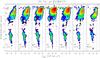 |
Fig. 1 Continuum-subtracted HST/STIS position-velocity (PV) plots of the jet from DG Tau, in [S ii]λ6731 emission in slit positions S1 to S7 (south-east to north-west). Contours are from 1.1 × 10⁻¹⁵ erg s-1 arcsec-2 cm-2 Å-1 (3σ), with a ratio of 22/5. The solid lines mark the position of the star and zero velocity, while dashed lines mark the positions of identified features in images of this flow (see text). |
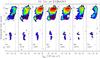 |
Fig. 2 Same as Fig. 1, but for [O ii]λ6363. The stronger doublet component, [O i]λ6300, is blue-shifted off the detector. However, since this doublet is emitted in a fixed ratio of 3:1, we use the [O i]λ6363 line in its place. |
At least three velocity components can be identified in the jet up to location A1: a low velocity component, between about −150 and +20, more evident in [S ii] and [O i], and in the lateral positions; a medium velocity component between −300 and −150 km s-1, more evident in [N ii], characterised by an emission peak at about 0.̋45 and a slow acceleration; and a high velocity component between about −300 and −400 km s-1, with an emission spot at 1.̋4, hereafter A1HV, brighter in slits 1, 2, 3 and 4, already identified as a knot in Lavalley-Fouquet et al. (2000) at 0.̋93 from the source. A bifurcation of the emission is evident between the low and the medium velocity components (e.g. slit 1 to 6 in [S ii] at A2, and slit 5 in [N ii] at 0.̋45). A steep gradient towards lower velocities, of ~30 km s-1, is apparent about 0.̋2 downstream from A1HV in [N ii], and less evidently in [S ii].
Futher along the jet, between A1 and ~3′′, emission is very low in [O i] and [S ii], while the [N ii] line is stronger, mainly at medium velocities. This region corresponds to a faint stripe connecting A1 and B1 in the images of Dougados et al. (2000). The PV plots are very difficult to read here, but there are indications of material flowing at two different velocities (about −150 and −320 km s-1), and marginal indications of a localised gradient in velocity (of about 30 km s-1) at 2.̋8.
Beyond 3′′, the system of slits intercepts the large (~2′′) bow-like feature of which B0 and B1 form a part. Here all lines are detected, with [N ii] being the strongest, but only at velocities between −150 and −350 km s-1, and brighter in slits S1 to S4. Another gradient towards lower velocities, of ~70 km s-1, is seen at 3.̋45 between the emission peaks at B0 and B1, and a less evident one at 4.̋1, of ~30 km s-1, downstream of knot B1. Interestingly, these apparent abrupt reductions in velocity occur immediately downsteam of a peak in emission. This is expected in radiative shocks, in which the discontinuity in velocity is at the front, while the optical emission arises behind the shock front on scales resolvable by HST (Hartigan et al. 1994).
3.2. Position-velocity diagrams of the line ratios
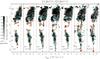 |
Fig. 4 Position-velocity plots of the [S ii]λ6731/[S ii]λ6716 line ratio in linear greyscale. Cyan and orange contours indicate the [S ii]λ6716 and [S ii]λ6731 emission at 3σ, respectively. Where only one of the two lines is above the 3σ threshold the upper/lower limit of the line ratio is reported. |
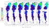 |
Fig. 5 Same as Fig. 4 for the logarithm of the [N ii](λ6583+λ6548)/ [O i](λ6300+λ6363) line ratio. The superposed cyan and red contours indicate the [O i]λ6363 and the [N ii]λ6583 emission at 3σ ([O i]λ6300 = 3 [OII]λ6363 and [N ii]λ6548 = 1/3 [N ii]λ6583 is assumed everywhere, see text). |
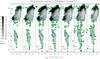 |
Fig. 6 Same as Fig. 4 for [O i](λ6300+λ6363)/[S ii](λ6716+λ6731) line ratio. Blue and green contours indicate [O i]λ6363 and the [S ii]6731+6716 emission at 3σ respectively. |
Figures 4–6 show emission line ratio PV plots for [S ii]31/16, [N ii]/[O i] and [O i]/[S ii], respectively. Plots are produced after two-pixel binning in both spatial and spectral dimensions, to reflect resolution (i.e. 0.̋1 and 50 km s-1). A 3σ contour (~2.2 × 10⁻¹⁵ erg s-1 arcsec-2 cm-2 Å-1 after binning) for each emission line is overlaid.
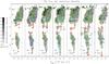 |
Fig. 7 Position-velocity plots of the logarithm of the electron density ne. Contours indicate regions inside which: cyan – [S ii]λ6716 ≥ 3σ; orange – [S ii]λ6731 ≥ 3σ; green – [S ii]31/16 ratio at the high density limit. Where only [S ii]λ6731 ([S ii]λ6731) ≥ 3σ, the derived ne is a lower (upper) limit. Inside the green contours ne is derived with the modified HDL-BE procedure (cf. Sect. 2.2). |
The [S ii] ratio is in many regions at the high density limit of 2.35 (HDL), beyond which the ratio is no longer a valid diagnostic tool. In these regions, encircled by green contours, the electron density is ≥2 × 104 cm-3, i.e. high when compared to published values at large distances along many jets of typically 103 cm-3.
The [N ii]/[O i] ratio is a good indicator of the hydrogen ionisation fraction since it increases monotonically with it, and is nearly independent of ne and Te, as long as the electron density is below the [N ii] critical electron density of ne< 105 cm-3. The value of this ratio is low near the star, but smoothly increases with distance and velocity. It reaches higher values at high speeds approaching A2, and at medium velocities between A2 and A1. At A1HV, both the [O i] and [N ii] lines are intense giving a moderate ratio. In the A1-B0 ridge the reported value of ~0.4 is a lower limit, as [O i] has been set to 3σ. Meanwhile, high ratio values return in the B0 - B1 region.
Finally, the [O i]/[S ii] line ratio depends on both ne and Te, and weakly on xe through [O i]. The ratio shows moderate values almost everywhere except for the shoulder between the star and A2 at progressively higher speeds, and at A1HV. This “shoulder” appears not to correspond to any of the kinematic components identified above.
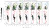 |
Fig. 8 Position-velocity diagrams of the ionisation fraction xe. Contours: blue – [O i]λ6363 at 3σ; red – [N ii]λ6583 at 3σ; green – high density limit for the [S ii]31/16 ratio. Where only [O i] ([N ii]) is above 3σ, xe is an upper (lower) limit. Inside the HDL regions xe is determined with the HDL-BE procedure (cf. Sect. 2.2). |
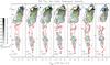 |
Fig. 9 Position-velocity diagrams of the logarithm of the hydrogen density derived as nH = ne/xe. Contour colour coding is as in Fig. 8. |
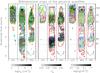 |
Fig. 10 2D velocity channel maps of the logarithm of the electron density (left), of the ionisation fraction (centre) and of the logarithm of the total density (right). Greyscales are linear. Low velocity interval (LVI) is defined as −120 to +25 km s-1, medium velocity interval (MVI) is defined as −270 to −120 km s-1 and high velocity interval (HVI) is defined as −420 to −270 km s-1. Contours: cyan – [S ii]λ6716 at 3σ; orange – [S ii]λ6731 at 3σ; green – region above [S ii] critical density; blue – [O i]λ6363 at 3σ; red – [N ii]λ6583 at 3σ. |
4. Results: physical quantities and jet widths
The diagnostic analysis was performed in three ways, in order to optimise the output and to facilitate comparisons with the literature. The first preserves all high resolution information in 3D (i.e. 2D space and 1D velocity), and the results are presented as PV plots of ne, xe, and nH (Figs. 7–9) giving a global picture of the jet excitation conditions. The results highlight regions of low signal-to-noise where the diagnostics would benefit from a further binning of the input data in space and/or velocity. Therefore, the second way of carrying out the analysis bins the velocity information into three velocity channels (Fig. 10), defined as low velocity interval (LVI), from −120 to +25 km s-1, medium velocity interval (MVI), from −270 to −120 km s-1 and high velocity interval (HVI) from −420 to −270 km s-1. The third way bins in velocity and jet width giving plasma parameters in 1D along the jet as it propagates (Figs. 11–13). 1D profiles of the line ratios are provided as on-line material, Figs. 16–18. In all cases, in positions in which the [SII] ratio is at the high density limit, the modified HDL technique has been applied (cf. Sect. 2.2) adopting in the affected regions Te = 104 K for the LVI, Te = 1 and 2 × 10⁴ K for the MVI, upstream and downstream A2, respectively, and Te = 3 × 10⁴ K for the HVI. Lastly, the jet width of the various velocity components is estimated, Fig. 14.
4.1. Electron density
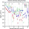 |
Fig. 11 1D profiles of log(ne) along the flow in discrete velocity intervals (see Fig. 10). Error bars (smaller than the symbol size where the signal is strong) are determined a posteriori by conducting the analysis with input values of the line ratios and their uncertainties (evaluated from the 3σ error on the fluxes). Empty symbols indicate positions where ne is above the high density limit of the [S ii] diagnostics, and the derivation has been made through the modified BE-technique described in Sect. 2.2. |
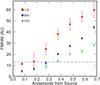 |
Fig. 14 DG Tau jet width in the first 0.̋7. Each point is the average obtained from four different lines, with the error bars indicating the dispersion. Dashed line: FWHM of the stellar continuum. |
The results for ne are illustrated in Figs. 7, 10 (left panels) and 11. The electron density is higher than 103 cm-3 almost everywhere in the jet (Fig. 7). The densest portion is near the jet base as far as A1, and for high velocities. While this trend was previously reported by Bacciotti et al. (2000) and Bacciotti (2002), these studies were limited by the critical density of [S ii]. Closer inspection via the modified BE-technique reveals that ne is higher in the MVI and HVI than in the LVI (Fig. 10), with values reaching close to 105 cm-3 near the star. Between the star and A2, there is marginal evidence of a separation between the LVI and the other velocity components (Fig. 7). Meanwhile, there is no variation of ne across the jet, from S1 to S7 in each velocity interval (Fig. 10).
Further along the jet, a slight increase in ne is noted at A1HV (Fig. 7), while downstream of A1, where the flow is seen only in the MVI and HVI, ne continues to decrease in the MVI, reaching 103 cm-3 at 2.̋8, in contrast to the HVI which reaches a maximum at this position. Continuing to the B0-B1 region, ne increases again in the MVI. Finally, the HVI contribution fades after B0, while in the MVI ne is detectable well beyond B1.
4.2. Ionisation fraction
The results for xe are illustrated in Figs. 8, 10 (middle panels) and 12. It is worth noting that the “missing” xe data points result from a low signal in both [S ii] lines, or lack of an unique solution from the code where [O i]/[S ii] ≫ 1 (i.e. between the star and A2). However, the trends in those regions can be gleaned from the [N ii]/[O i] ratio (Fig. 5), which is almost directly proportional to xe.
At the base of the jet, xe is not larger than 0.07 (Fig. 8), but it increases with distance and velocity up to a high value of over 0.6 in the region between A2 and A1, peaking at different distances in each velocity interval. Before A1, xe drops in MVI and HVI, while in LVI it increases toward A1 (Fig. 8). There is no strong enhancement of xe at A1HV, contrary to what would be expected given the strong emission. Moving along the jet, we note that between A1 and B0 the determination of xe is poor, and given often in terms of lower limits. Binning over space and velocity increases the [O i] signal-to-noise, making more evident the existence of a high ionisation region between 2′′ and 4.̋1 in both the MVI and the HVI. In the 1D profiles xe shows a plateau in xe of ~0.7 in this region. At 3.̋9 a sharp drop occurs for the MVI, possibly coincident with the 30 km s-1 velocity gradient (Sect. 3.1). After this point one sees a more gradual decrease in xe, for the MVI, represented mainly by lower limits (Fig. 12). Finally, as for ne, no large transverse variations are evident in the velocity channel maps of xe (Fig. 10).
4.3. Total hydrogen density
The results for nH are illustrated in Figs. 9, 10 (right panels) and 13. We stress that our mapping of this quantity is more extended than in previous works, thanks to the application of the modified BE-technique. Similar to ne, the total hydrogen density is at its maximum of 3 × 106 cm-3 close to the star, and then decreases by several orders of magnitude along the flow. The range of variation is larger than in ne, because of the effect of the increase in ionisation. Again, no spatial variation is evident in the transverse direction.
In contrast to MVI and LVI trends, moving from A2 to A1 we see a plateau in nH for HVI, giving rise to the high emission of the AHV1 spot. Then nH drops back again downstream of A1HV (Fig. 13). Other nH increases in HVI followed by a drop are seen at 2.̋8 and at B0 and B1. We note that all these locations are also sites of velocity gradients (Sect. 3.1) and this coincidence points toward a shock nature of the exciting mechanism, as it is dicussed in Sect. 5.2. At B0, the HVI jet slows down and merges with the MVI component, that remains dense to beyond B1 (Fig. 10).
4.4. Jet width in the initial channel
Measurements of the jet width close to its base are useful in constraining models for launching jets. We estimate the jet width, for the first 0.̋7 of the flow, as the full-width-half-maximum (FWHM) of the intensity profile across the jet. The intensity profiles are obtained by using the seven slit positions to construct an image of the jet in each of four emission lines ([O i]λ6563, [N ii]λ6583, [S ii]λ6716, [S ii]λ6731), and in three velocity intervals (similar to Fig. 10). The measured FWHM is deconvolved by subtracting in quadrature the FWHM of a reconstructed image of the stellar continuum in a wavelength interval of 3.2 Å, which turns out to be 13 AU (due to the overlap of the slit width).
The jet width estimates are shown in Fig. 14, where each point is the average of the values obtained in the different lines in each of the velocity intervals (with the error bar indicating the dispersion). The magnitude of the opening angle of the jet depends on the velocity interval, with the LVI being wider and the HVI narrower. However, within each velocity interval, the slope remains almost constant.
Our results for the jet width are in agreement with the values estimated in Dougados et al. (2000) and Woitas et al. (2002), where these velocity-integrated results are close to our MVI values. In a recent infra-red study of the DG Tau jet Agra-Amboage et al. (2011), the [Fe ii] emission at velocities of −300 to −160 km s-1 appears to have a smaller opening angle than our corresponding MVI emission, but similar to our HVI emission. This difference may be due to variability of the flow over a six year interval. For example, the data in Agra-Amboage et al. (2011) may have been taken between two episodes of intermittent inflation of hot plasma close to the source. Indeed, in contrast to our spectra, the [Fe ii] emission did not show any emission at velocities above −300 km s-1. Monitoring of [Fe ii] emission over time intervals of 1–2 years would help clarifying this issue.
5. Discussion
5.1. Flow structure
The emerging picture is that of a flow initially collimated and characterised by smoothly varying properties, which soon undergoes strong perturbations represented by bright spots in the PV plots corresponding to the tips of the bow-like features described by Bacciotti et al. (2000) and Lavalley et al. (1997).
The initial jet channel, up to at least position A2, has characteristics consistent with an overall onion-like kinematic structure, like the one predicted by classical models of jet launching, such as the so-called Disk-wind (e.g. Ferreira et al. 2006; Pudritz et al. 2007) or X-wind (Shu et al. 2000; Shang et al. 2002). In this context an interesting aspect is the apparent acceleration of the gas between the star and A2. Magnetocentrifugal models of disk winds predict an acceleration to asymptotic velocities on a scale proportional to the footpoint radius, r0 (i.e. the radius from the star in the disk plane from which the jet is launched). The terminal speed is reached at about 1000r0 for the solutions in Garcia et al. (2001, cf. their Fig. 1) and at about 100r0 for the solutions in Pesenti et al. 2004. Our observed acceleration would then imply a launch radius of 0.3 or 3 AU, respectively. Alternatively, the ejection velocity has decreased over time, or the apparent acceleration is actually the effect of the superposition of separate components.
Pyo03 examine the jet structure at lower spatial resolution in [Fe ii] infra-red emission. Two well-separated velocity components are detected at epoch 10/2001. Their low radial velocity component of −80 km s-1, located at 0.̋4, may correspond to the bright spot seen at the stellar position in our LVI, while their “high radial velocity component” at −220 km s-1, located at 0.̋6–0.̋8, may correspond to the bright elongated feature seen in our MVI in the [N ii] PV plots at 0 to 0.̋4 from the star. No HVI material is reported in Pyo et al. (2003), but the A1HV feature would have moved out of their 1.̋6-long diagrams in two years.
5.2. Gas heating
While our results are in agreement with previous studies, such as Lavalley-Fouquet et al. (2000), our analysis improves on these studies by quantifying the higher jet densities in the region close to the star.
In addition, the HST resolution reveals that the ionisation peaks upstream A1 have different positions in the different velocity bins (0.̋8 for the HVI, 1.̋1 for the MVI, and 1.̋4 for LVI, with a smaller peak at 0.̋5), followed by a decrease. This behaviour is reminiscent of the excitation produced by a Disk-wind heated by ambipolar diffusion (Garcia et al. 2001, Figs. 1, 2). In this model the slower outer material reaches its maximum xe at a greater distance than the inner higher velocity gas. The xe value, however, is much smaller than our value at the observed location. Alternatively, the HVI and MVI xe peaks may be due to marginally resolved shocks which are not evident in the forbidden emission lines. Indeed, in Bacciotti et al. (2000), small condensations are visible at 0.̋5 and 1.̋1 but only in the strong Hα line, in reconstructed images at various velocities. This would be in line with the conclusions of Lavalley-Fouquet et al. (2000), who find that the observed [N ii]/[O i] ratio are compatible only with shock heating, and of the numerical study of Massaglia et al. (2005), where the variations of xe and ne in distance were reproduced by a continuous series of identical shocks travelling along a jet of decreasing density.
We stress that we see an increase in total density nH toward each knot, at the same location of a sharp velocity gradient. This is a key result as these sudden compressions indicate clearly that the luminous knots in the DG Tau jet are generated by propagating shock fronts. For example, at A1HV, the high velocity tip of the A1 structure, there is a velocity gradient associated to a high nH value in the HVI. Then at B0, the velocity jump and the local increase in density suggests that this knot is shocking the slower gas at B1. Again feature B1 has the properties expected for a shock front generated by higher velocity gas catching up with slower material emitted at an earlier time. At 4.̋1, just downstream of the B1 emission peak, we see a supersonic velocity jump associated with a gradient in density and ionisation.
The increase in total density in proximity to velocity jumps, however, does not always correspond to an increase in ionisation. At A1HV, for example, no peak in xe is found. Again at B0 one would expect an increase in ionisation, but xe was already high upstream of B0. Spatial offsets between the position of peaks in xe and the position of shock fronts have been found in other works conducted on similar spatial scales (see e.g. Hartigan & Morse 2007 for the HH 30 jet). The lack of variation in xe does not necessarily exclude a shock. In a number of cases, in fact, line ratio modelling has shown evidence of substantial pre-shock ionisation (see, e.g., Hartigan et al. 2004, in HN Tau jet and Teşileanu et al. 2012, for the jet from RW Aur). If a strong pre-shock ionisation was created, for example by the passage of a previous front, or by the x-ray field associated with this jet (Güdel et al. 2011), this ionisation could endure in a low density gas because of the slow recombination time (Bacciotti et al. 1999). The half-life of free electrons is given by trec = (neαH(Te))-1, where α is the hydrogen recombination coefficient (which is weakly dependent on Te). Taking αH = 2.5 × 10⁻¹³ cm3 s-1 (Osterbrock 1989) and for the HVI upstream of B0 ne = 7 × 103 cm-3, we obtain a recombination time of trec = 6 × 10⁸ s. Combining this with a radial velocity of −300 km s-1 and the jet inclination of 38° to the line of sight, we find that the free electrons can travel a distance of about 3′′ in the plane of the sky before recombination.
Finally, all PV plots show a slight asymmetry with respect to the axis. This jet wiggle was first detected by Dougados et al. (2000), and is clear in Fig. 10 in the faint region between A1 and B0. Following Lavalley-Fouquet et al. (2000), the wiggling may explain the high excitation in this region, as a bending of the jet by only 10° at the observed velocities can produce oblique fronts with shock speeds of up to 70 km s-1.
5.3. Mass outflow rate
An important parameter in any jet launching model is the mass outflow rate. To ensure accuracy in estimates, it is vital to make measurements as close as possible to the base of the jet. Here it is hoped that the plasma parameters are still dominated by the physics of the launching mechanism, rather than interactions with the environment through which it propagates. Our HST/STIS dataset allows us to estimate the mass outflow rate of the jet, Ṁj, for the first 0.̋7 from the star. Inspired by the magneto-centrifugal models (Cabrit et al. 1999; Pudritz et al. 2007; Shang et al. 2002), we assume that the jet flows along nested magnetic surfaces, with a poloidal velocity which decreases with distance from the jet axis. Based in Fig. 14, the flow is structured in three nested cones around a hollow core, with boundary surfaces labelled k = 1–4 according to increasing opening angle. Therefore, k = 2–4 mark the outer surfaces of the HVI, MVI and LVI jet cones, respectively. Once the jet reaches a distance, d, of 50 AU above the disk plane, the k = 1 surface opens out to a diameter of either 6 AU for the disk-wind (Cabrit et al. 1999) or 2 AU, for the X-wind model (Shang et al. 2002).
At each distance, d, the jet material of each cone crosses an annulus of area  , where rk(d) = FWHM(d)/2 is the radius of a given cone surface. We define αk as half of the opening angle of a given cone. From Fig. 14, we find that αk = 8°,11°,19° for k = 2,3,4, respectively, and αk< 3° for k = 1 if we consider the Disk-wind model. The mass flux Ṁj in each velocity interval, labelled by the outer cone surface k of that interval, is then given by
  (1)where nH,k is the hydrogen density in the velocity interval region (with values taken from Fig. 13), μ = 1.41 is the average atomic weight per hydrogen atom (Allen & Cox 2001), mp the proton mass, i = 38° is the jet inclination angle with respect to the line of sight, and βk = (αk + αk − 1)/2. In the above expression,
  is the module of the average poloidal velocity in the considered interval, given as
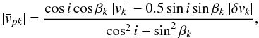 vk is the radial velocity at the middle of the interval and δvk the width of the velocity interval. Finally, fc is a correction factor which accounts for compression of the flow in unresolved shocks, estimated as the square root of the inverse of the post-shock compression (Hartigan et al. 1994). The latter is found to be 8–10 after 10 years evolution for an average shock velocity around 50 km s-1 and pre-shock magnetic field around 100 μG, (Massaglia et al. 2005), leading to fc = 1/3.
The results for α1 = 3° (i.e. the Disk-wind model) are presented in Fig. 15.
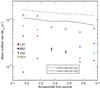 |
Fig. 15 Mass outflow rate of the jet, Ṁj, using two methods: (i) jet density traversing annuli of nested cones, represented by data points broken down by velocity interval and also totalled; (ii) jet density obtained via emission line luminosities from a uniform slab, as in Hartigan et al. (1995), represented by curves. Uncertainties are about 50% in every velocity interval. |
Neglecting the errors on distance and inclination, the uncertainty arises in the density and FWHM estimates. On average the uncertainty is of 20%, 30%, and 40% for the HVI, MVI, and LVI mass loss rates, respectively, as well as an additional 20 to 30% error introduced by the modified BE-technique for the MVI and HVI densities. The net effect is an uncertainty of 50% in every velocity interval.
Figure 15 shows that the contribution of the LVI and HVI is dominant initially, but it decreases with distance by 75%, due to the fall of density. By contrast, the MVI contribution increases beyond the LVI and HVI contributions from 0.̋5. The average total mass outflow rate of the jet is Ṁj = 8 ± 4 × 10⁻⁹ M⊙ yr-1, slightly decreasing with distance which is probably due to flux falling outside the 0.̋5 slit coverage as the jet diverges. Assuming a smaller central hollow cone, as in the X-wind model, only the HVI contribution increases, to a maximum of 25% for α1 = 0. Since the data are flux-calibrated, Ṁj could also be estimated using the luminosity-based method of Hartigan et al. (1995), finding good agreement (Fig. 15).
The derived  values of 10-9 to 10-8 match typical values for jets from CTTSs (e.g. for RW AUR Ṁj ~ 4.6 × 10⁻⁹ M⊙ yr-1Melnikov et al. 2009; and in CW Tau Ṁj ~ 7 × 10⁻⁹ M⊙ yr-1Coffey et al. 2008), and compare well with previous estimates for DG Tau. At 0.̋3 from the star, Coffey et al. (2008) find Ṁj = 2.6 and 4.1 × 10⁻⁸ M⊙ yr-1 at −100 and −225 km s-1. These values are reconciled with ours by: applying FWHM deconvolution (i.e. yielding jet widths of 24 and 15 AU, respectively); replacing the unreliable value for xe at high velocity; and introducing fc = 1/3. Meanwhile, Agra-Amboage et al. (2011) obtain a value of Ṁj ~ 1.6 and 1.7 × 10⁻⁸ M⊙ yr-1 at −300 and −135 km s-1. Their “jet density and cross-section” method at 0.̋4–0.̋7 (their Fig. 9) gives results in agreement with ours, if fc = 1/3 is applied. Finally, Lavalley-Fouquet et al. (2000) reported Ṁj ~ 0.2, 0.8, and 0.4 × 10⁻⁸ M⊙ yr-1 in their LVI, MVI, and HVI components beyond 1.̋2 from the star, again in line with our estimates.
Given that the range of accretion rates prevailing in DG Tau is found to be Ṁacc = 3 ± 2 10-7 M⊙ yr-1 (Agra-Amboage et al. 2011), for the two-sided jet the ejection to accretion ratio Ṁj/Ṁacc turns out to vary between 0.03 ± 0.01 and 0.16 ± 0.08, which is compatible with the range predicted by Disk-wind models (e.g. 0.01 <Ṁj/Ṁacc< 0.2, Ferreira et al. 2006).
5.4. Angular momentum flux
In these spectra Bacciotti et al. (2002) found systematic differences in the Doppler shift of the LVI emission either side of the jet axis. These measurements were tentatively interpreted as the jet rotating about its axis as it propagates. Toroidal velocities were found to be ~5–20 km s-1 at a radius of 20–30 AU from the jet axis and a distance of 40–80 AU from the star-disk plane. Subsequently, similar differences in Doppler shift were detected in this and other jets (Coffey et al. 2004; Woitas et al. 2005; Coffey et al. 2007). These results seem to support magneto-centrifugal jet launch and, in particular, the fact that jets extract the excess angular momentum from the star-disk system. Our estimate of Ṁj now enables us to test the extraction efficiency. We approximate the angular momentum of the jet in a given velocity interval (where k labels the outer cone surface of that interval) as follows: 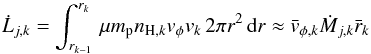 (2)where vk and vφ are the poloidal and toroidal components of the jet velocity. In DG Tau, vφ could only be measured for LVI and MVI (Bacciotti 2002; Coffey et al. 2007), so Eq. (2) simplifies to
  (3)where
  and
and  + rk−1)/2, for k = 3,4 respectively. Given vφ ~ 15 ± 5 km s-1 for DG Tau at 0.̋3 from the star (Coffey et al. 2007), and taking the values of mass outflow rates and FWHMs (with their error) derived at this distance, we obtain
  and 1.2 ± 0.8 × 10⁻⁷ M⊙ yr-1 AU km s-1 for the LVI and MVI components, respectively . The difference with higher values given by Bacciotti et al. (2002) and Coffey et al. (2008),
  and 1.3 × 10⁻⁵ M⊙ yr-1 AU km s-1, respectively, arises because we calculate lower mass outflow rates and smaller radii. Ferreira et al. (2006), however, show that for DG Tau at 50 AU from the star, the outer streamlines of the wind have not yet reached the asymptotic regime and contain only half of their final angular momentum, contrary to the inner streamlines. Accounting for this effect and for the presence of a symmetric red-shifted jet we obtain globally
  yr-1 AU km s-1.
In order to allow accretion to proceed, the disk must loose angular momentum. The excess angular momentum to be removed from the disk,  , can be calculated as in Woitas et al. (2005), Sect. 4.2. We consider a Disk-wind launched at a broad range of disk radii, from the innermost region where the disk is truncated by the stellar magnetosphere at rin ~ 0.03 AU, to the outermost region at rout ~ 3 AU (the latter value is dictated by limiting poloidal velocities of 50 km s-1, Bacciotti et al. 2002; Anderson et al. 2003; Pesenti et al. 2004). The disk material falling below the inner radius is accreted in full onto the star, such that the disk mass flux at the inner radius ṀD,in is equal to Ṁacc, the mass accretion flux. Conservation of mass in the disk dictates that the mass flux in the disk at the outer radius, ṀD,out, satisfies ṀD,out = Ṁacc + 2Ṁj. Considering the range of Ṁacc found in DG Tau and the estimate of Ṁj reported in the previous section, we obtain ṀD,out = 3.2 ± 2.1 × 10⁻⁷ M⊙ yr-1. The angular momentum which the disk looses between the outer and inner radii is given by
  (4)where vK is the Keplerian velocity of the disk. With M⋆ = 0.5 M⊙, vK = 122 and 11 km s-1 at the inner and outer radii, respectively, and therefore
  yr-1 AU km s-1. and are of the same order of magnitude, and both present a wide range of variation. It cannot be excluded that the atomic jet is carrying away all the excess angular momentum from the disk out to 3 AU, if the accretion rate was at the low end of the range of Ṁacc measured for DG Tau over the period 1988–2003 (Agra-Amboage et al. 2011). Unfortunately, however, the large uncertainties still affecting the mass outflow and accretion rates prevent a firm conclusion on this point.
6. Summary and conclusions
We analysed a set of seven high angular resolution HST/STIS spectra of the first 5 arcseconds of the outflow from DG Tau, taken in January 1999 with spectral and spatial resolution of ~50 km s-1 and 0.̋1. Previously published results based on this extraordinarily rich dataset include: the basic morphology of the jet in the first 2′′ from the star (Bacciotti et al. 2000); a preliminary set of spectral diagnostics over the same region (Bacciotti 2002); indications of jet rotation (Bacciotti et al. 2002). Here, we continue to exploit the 1999 HST/STIS dataset, to achieve a high resolution parameterisation of the jet plasma physics, investigating it in three dimensions: along the first 5′′of the jet; across the jet width; and in velocity space. We provide the PV plots of the forbidden emission lines and their ratios. From these we derive PV plots of the electron density ne, hydrogen ionisation fraction xe, and total hydrogen density nH, by applying an updated version of the BE-technique (first published in Bacciotti et al. 1999). The presentation of the results as PV plots has the advantage of retaining all the spatio-kinematic information available. To assist with the interpretation, we also create 2D images, and 1D profiles along the jet, of the plasma parameters in each of three velocity intervals, defined as LVI from −120 to +25 km s-1, MVI from −270 to −120 km s-1 and HVI from −420 to −270 km s-1, applying the updated technique to binned data. Our main conclusions are listed below.
Within the first arcsecond, the flow presents smoothly varying kinematic properties, with an apparent continuous acceleration in [S ii] and [O i] PV plots, reminiscent of a magneto-centrifugal jet launch mechanism. The [N ii] emission is concentrated in medium to high velocities, and the identified features in the flow (A2, A1, B0, B1) are associated with supersonic velocity jumps as expected of shocked gas. Previous reports of an onion-like kinematic structure in the initial (first 1′′) channel are confirmed, but the new estimates of the jet excitation properties indicate that the efficiency of their ionising mechanism is different in the moderate-high velocity components of the flow with respect to the surrounding slower, wider flow.
To find the plasma parameters above the high density limit of [S ii], the modified BE-technique was applied. At the beginning of the jet, values up to ne ~ 105 cm-3 were found for MVI and HVI, while lower values of ne ~ 104 cm-3 were found in the LVI. In the same region, xe increases markedly in the MVI and HVI, up to values of 0.7 and 0.6, respectively, close to A2. By contrast, the LVI value remains low i.e. xe ≤ 0.3 within the location of A1. This suggests a fundamental difference between the dominant ionisation process in the MVI and HVI components with respect to the LVI component. Proceeding along the jet beyond feature A1, ne decreases in all velocity intervals. Meanwhile, xe is found to remain high (0.7–0.8) in the MVI and HVI (the LVI is not visible here), both in the A2-B0 stream, and between features B0 and B1. After B1, ne and xe can only be determined for the MVI, and both decrease to low values, along the jet to 5 ′′. The total hydrogen density nH for the three velocity intervals is similar within a factor 3–4 all along the jet. Beyond A1 we have no nH estimates for the LVI, but values similar to our HVI are found here by Lavalley-Fouquet et al. (2000). Overall, the total density drops in magnitude over 4 orders along the jet (from almost 107 to 103 cm-3). Our results are in agreement with previous determinations of the excitation parameters, in the regions where the comparison was feasible.
Remarkably, our analysis shows absence of significant variations in the plasma parameters across the jet width in each velocity interval. Slightly downstream the emission peaks at AHV1, B0 and B1, and in the HVI, local pronounced gradients of the total density are found to be coincident with velocity jumps. This is direct evidence that the gas is compressed locally at the position of sharp velocity gradients, supporting a shock origin for the observed knots, as proposed by Lavalley-Fouquet et al. (2000). This conclusion holds true even if not in all cases an increase in ionisation is detected at the velocity jumps, as it is in the MVI at B1. In fact the absence of variation in the ionisation level does not exclude a shock, as the ionisation created by the passage of a previous shock or by a radiation field could endure because of the slow recombination time in a rarefied medium (Bacciotti et al. 1999). We confirm reports of wiggling between A1 and B0, supporting the suggestion by Lavalley-Fouquet et al. (2000), that the high excitation values in this region may be maintained via the occurence of lateral shocks.
The mass outflow rate of the jet, , is found as a function of velocity and distance from the star, in the initial portion of the jet (0.̋1–0.̋7), using the jet density and cross-section measurements. is similar in the HVI and LVI, and decreases along the flow. Meanwhile, the MVI value is initially lower, but then increases with distance until it dominates after 0.̋5. The total mass flux, of all velocity intervals, is on average  yr-1, and it is found to decrease slightly with distance, but this could be a bias introduced by the line flux loss at the slit borders. Results were cross-checked with mass outflow rates obtained via emission line luminosity (cf. Hartigan et al. 1995), finding good agreement. Taking into account differences in the derivation procedure, our results are also in agreement with previous estimates for this jet, and in the typical range for CTTS jets. Given the range of mass accretion rates found in DG Tau of Ṁacc ~ (3 ± 2) × 10-7 M⊙ yr-1 (Agra-Amboage et al. 2011), the ratio of mass ejection to mass accretion, Ṁj/Ṁacc, for the supposedly simmetric bipolar jet can vary between 0.03 ± 0.01 and 0.16 ± 0.08, which is compatible with the range predicted by Disk-wind models.
Combining the derived mass outflow rates with previously published toroidal velocities for the LVI and MVI material at 0.̋3 form the star, we estimate the angular momentum transported by these components. Considering two symmetric jet lobes and allowing a correction for the fraction of the angular momentum still in the disk-wind magnetic field before the asymptotic regime is reached, turns out to be ~(2.9 ± 1.5) × 10-6 M⊙ yr-1 AU km s-1. We tentatively compare this estimate to the amount of angular momentum lost by the disk to allow accretion, . Proceeding as in Woitas et al. (2005), we find yr-1 AU km s-1, which indicates that the two quantities are of the same order of magnitude, and comparable if the accretion rate was at its lower values when the material probed by our data was ejected. The large uncertainties affecting both estimates, however, prevent further conclusions.
In summary, the physical structure of the DG Tau jet reveals patterns of variation in parameters which are expected of magneto-centrifugal jet launch models. However, the situation is complicated by the simultaneous presence of other features, like hints of a multi-component flow, and shock fronts formed on different temporal scales, which seem to reach beyond this simple scenario. The presented plasma maps constitute a powerful benchmark for testing new alternatives.
Online material
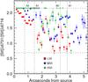 |
Fig. 16 1D profile of the [S ii]31/16 ratio along the flow, derived from integration of the line surface brightness across the jet and over each velocity interval. Horizontal dashed lines indicate upper and lower density limits on validity of the ratio as a ne diagnostic. Empty symbols mark positions and velocities for which the modified BE-technique has been applied. Upper and lower limits arise when one of the lines is undetected, and so its flux has been set to 3σ. |
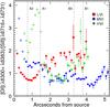 |
Fig. 18 Same as Fig. 16 for the [O i]/[S ii] line ratio. Due to the prominence of [O i] emission over the [S ii] lines close to the star, a few points are off the scale. Their values are: 6.58 at 0.̋175, for the MVI, and 12.10, 14.49, 9.54 and 4.99 at 0.̋175, 0.̋275, 0.̋375 and 0.̋475, respectively, for the HVI. |
Acknowledgments
The authors wish to thank the referee, Sylve Cabrit, for her detailed and thorough reports, that led to a significant improvement in the derivation and presentation of the results. L.M. thanks S. Cabrit and C. Dougados for the hospitality at IAP during the preliminary analysis of the data. T.P.R. acknowledges support from Science Foundation Ireland under grant 07/RFP/PHYF790.
References
- Agra-Amboage, V., Dougados, C., Cabrit, S., & Reunanen, J. 2011, A&A, 532, A59 [NASA ADS] [CrossRef] [EDP Sciences] [Google Scholar]
- Allen, C. W., & Cox, A. N. 2001, Allen’s astrophysical quantities, 4th edn. (Springer), 729 [Google Scholar]
- Anderson, J. M., Li, Z.-Y., Krasnopolsky, R., & Blandford, R. D. 2003, ApJ, 590, L107 [NASA ADS] [CrossRef] [Google Scholar]
- Asplund, M., Grevesse, N., & Sauval, A. J. 2005, in Cosmic Abundances as Records of Stellar Evolution and Nucleosynthesis, eds. T. G. Barnes, III, & F. N. Bash, ASP Conf. Ser., 336, 25 [Google Scholar]
- Bacciotti, F. 2002, in Rev. Mex. Astron. Astrof. Conf. Ser. 13, eds. W. J. Henney, W. Steffen, L. Binette, & A. Raga, 8 [Google Scholar]
- Bacciotti, F., & Eislöffel, J. 1999, A&A, 342, 717 [NASA ADS] [Google Scholar]
- Bacciotti, F., Eislöffel, J., & Ray, T. P. 1999, A&A, 350, 917 [NASA ADS] [Google Scholar]
- Bacciotti, F., Mundt, R., Ray, T. P., et al. 2000, ApJ, 537, L49 [NASA ADS] [CrossRef] [Google Scholar]
- Bacciotti, F., Ray, T. P., Mundt, R., Eislöffel, J., & Solf, J. 2002, ApJ, 576, 222 [NASA ADS] [CrossRef] [Google Scholar]
- Bally, J., Reipurth, B., & Davis, C. J. 2007, Protostars and Planets V, 215 [Google Scholar]
- Berrington, K. A., & Burke, P. G. 1981, Planet. Space Sci., 29, 377 [NASA ADS] [CrossRef] [Google Scholar]
- Cabrit, S. 2009, in Protostellar Jets in Context, eds. K. Tsinganos, T. Ray, & M. Stute (Berlin: Springer), Ap&SS Proc. Ser., 247 [Google Scholar]
- Cabrit, S., Ferreira, J., & Raga, A. C. 1999, A&A, 343, L61 [Google Scholar]
- Cerqueira, A. H., Velázquez, P. F., Raga, A. C., Vasconcelos, M. J., & de Colle, F. 2006, A&A, 448, 231 [NASA ADS] [CrossRef] [EDP Sciences] [Google Scholar]
- Coffey, D., Bacciotti, F., Woitas, J., Ray, T. P., & Eislöffel, J. 2004, Ap&SS, 292, 553 [NASA ADS] [CrossRef] [Google Scholar]
- Coffey, D., Bacciotti, F., Ray, T. P., Eislöffel, J., & Woitas, J. 2007, ApJ, 663, 350 [NASA ADS] [CrossRef] [Google Scholar]
- Coffey, D., Bacciotti, F., & Podio, L. 2008, ApJ, 689, 1112 [NASA ADS] [CrossRef] [Google Scholar]
- De Colle, F., del Burgo, C., & Raga, A. C. 2010, ApJ, 721, 929 [NASA ADS] [CrossRef] [Google Scholar]
- Dougados, C., Cabrit, S., Lavalley, C., & Ménard, F. 2000, A&A, 357, L61 [NASA ADS] [Google Scholar]
- Edwards, S. 2009, in 15th Cambridge Workshop on Cool Stars, Stellar Systems, and the Sun, ed. E. Stempels, AIP Conf. Ser., 1094, 29 [Google Scholar]
- Eislöffel, J., & Mundt, R. 1998, AJ, 115, 1554 [NASA ADS] [CrossRef] [Google Scholar]
- Ferreira, J., Dougados, C., & Cabrit, S. 2006, A&A, 453, 785 [NASA ADS] [CrossRef] [EDP Sciences] [Google Scholar]
- Garcia, P. J. V., Cabrit, S., Ferreira, J., & Binette, L. 2001, A&A, 377, 609 [NASA ADS] [CrossRef] [EDP Sciences] [Google Scholar]
- Güdel, M., Skinner, S. L., Audard, M., Briggs, K. R., & Cabrit, S. 2008, A&A, 478, 797 [NASA ADS] [CrossRef] [EDP Sciences] [Google Scholar]
- Güdel, M., Audard, M., Bacciotti, F., et al. 2011, in ASP Conf. Ser. 448, eds. C. Johns-Krull, M. K. Browning, & A. A. West, 617 [Google Scholar]
- Hartigan, P., & Morse, J. 2007, ApJ, 660, 426 [NASA ADS] [CrossRef] [Google Scholar]
- Hartigan, P., Morse, J. A., & Raymond, J. 1994, ApJ, 436, 125 [NASA ADS] [CrossRef] [Google Scholar]
- Hartigan, P., Edwards, S., & Ghandour, L. 1995, ApJ, 452, 736 [NASA ADS] [CrossRef] [Google Scholar]
- Hartigan, P., Edwards, S., & Pierson, R. 2004, ApJ, 609, 261 [NASA ADS] [CrossRef] [Google Scholar]
- Hartmann, L., & Raymond, J. C. 1989, ApJ, 337, 903 [NASA ADS] [CrossRef] [Google Scholar]
- Hudson, C. E., & Bell, K. L. 2005, A&A, 430, 725 [NASA ADS] [CrossRef] [EDP Sciences] [Google Scholar]
- Keenan, F. P., Aller, L. H., Bell, K. L., et al. 1996, MNRAS, 281, 1073 [NASA ADS] [Google Scholar]
- Kwan, J., & Tademaru, E. 1988, ApJ, 332, L41 [NASA ADS] [CrossRef] [Google Scholar]
- Lavalley, C., Cabrit, S., Dougados, C., Ferruit, P., & Bacon, R. 1997, A&A, 327, 671 [NASA ADS] [Google Scholar]
- Lavalley-Fouquet, C., Cabrit, S., & Dougados, C. 2000, A&A, 356, L41 [NASA ADS] [Google Scholar]
- Massaglia, S., Mignone, A., & Bodo, G. 2005, A&A, 442, 549 [NASA ADS] [CrossRef] [EDP Sciences] [Google Scholar]
- McGroarty, F., Ray, T. P., & Froebrich, D. 2007, A&A, 467, 1197 [NASA ADS] [CrossRef] [EDP Sciences] [Google Scholar]
- Melnikov, S., Woitas, J., Eislöffel, J., et al. 2008, A&A, 483, 199 [NASA ADS] [CrossRef] [EDP Sciences] [Google Scholar]
- Melnikov, S. Y., Eislöffel, J., Bacciotti, F., Woitas, J., & Ray, T. P. 2009, A&A, 506, 763 [NASA ADS] [CrossRef] [EDP Sciences] [Google Scholar]
- Mendoza, C. 1983, in Planetary Nebulae, ed. D. R. Flower, IAU Symp., 103, 143 [Google Scholar]
- Mundt, R., & Fried, J. W. 1983, ApJ, 274, L83 [NASA ADS] [CrossRef] [Google Scholar]
- Osterbrock, D.E., 1989, Astrophysics of Gaseous Nebulae and Active Galactic Nuclei (Mill Valley, CA: University Science Books) [Google Scholar]
- Pesenti, N., Dougados, C., Cabrit, S., et al. 2004, A&A, 416, L9 [NASA ADS] [CrossRef] [EDP Sciences] [Google Scholar]
- Podio, L., Bacciotti, F., Nisini, B., et al. 2006, A&A, 456, 189 [NASA ADS] [CrossRef] [EDP Sciences] [Google Scholar]
- Podio, L., Eislöffel, J., Melnikov, S., Hodapp, K. W., & Bacciotti, F. 2011, A&A, 527, A13 [NASA ADS] [CrossRef] [EDP Sciences] [Google Scholar]
- Pudritz, R. E., Ouyed, R., Fendt, C., & Brandenburg, A. 2007, Protostars and Planets V, 277 [Google Scholar]
- Pyo, T.-S., Kobayashi, N., Hayashi, M., et al. 2003, ApJ, 590, 340 [NASA ADS] [CrossRef] [Google Scholar]
- Ray, T., Dougados, C., Bacciotti, F., Eislöffel, J., & Chrysostomou, A. 2007, Protostars and Planets V, 231 [Google Scholar]
- Raymond, J. C., Morse, J. A., Hartigan, P., Curiel, S., & Heathcote, S. 1994, ApJ, 434, 232 [NASA ADS] [CrossRef] [Google Scholar]
- Safier, P. N. 1993, ApJ, 408, 148 [NASA ADS] [CrossRef] [Google Scholar]
- Shang, H., Glassgold, A. E., Shu, F. H., & Lizano, S. 2002, ApJ, 564, 853 [NASA ADS] [CrossRef] [Google Scholar]
- Shu, F. H., Najita, J. R., Shang, H., & Li, Z.-Y. 2000, Protostars and Planets IV, 789 [Google Scholar]
- Takami, M., Chrysostomou, A., Bailey, J., et al. 2002, ApJ, 568, L53 [NASA ADS] [CrossRef] [Google Scholar]
- Teşileanu, O., Mignone, A., Massaglia, S., & Bacciotti, F. 2012, ApJ, 746, 96 [NASA ADS] [CrossRef] [Google Scholar]
- Whelan, E. T., Ray, T. P., Bacciotti, F., et al. 2005, Nature, 435, 652 [NASA ADS] [CrossRef] [PubMed] [Google Scholar]
- Woitas, J., Ray, T. P., Bacciotti, F., Davis, C. J., & Eislöffel, J. 2002, ApJ, 580, 336 [NASA ADS] [CrossRef] [Google Scholar]
- Woitas, J., Bacciotti, F., Ray, T. P., et al. 2005, A&A, 432, 149 [NASA ADS] [CrossRef] [EDP Sciences] [Google Scholar]
All Figures
|
Fig. 1 Continuum-subtracted HST/STIS position-velocity (PV) plots of the jet from DG Tau, in [S ii]λ6731 emission in slit positions S1 to S7 (south-east to north-west). Contours are from 1.1 × 10⁻¹⁵ erg s-1 arcsec-2 cm-2 Å-1 (3σ), with a ratio of 22/5. The solid lines mark the position of the star and zero velocity, while dashed lines mark the positions of identified features in images of this flow (see text). |
| In the text | |
|
Fig. 2 Same as Fig. 1, but for [O ii]λ6363. The stronger doublet component, [O i]λ6300, is blue-shifted off the detector. However, since this doublet is emitted in a fixed ratio of 3:1, we use the [O i]λ6363 line in its place. |
| In the text | |
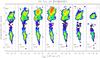 |
Fig. 3 Same as Fig. 1, but for [N ii]λ6583. |
| In the text | |
|
Fig. 4 Position-velocity plots of the [S ii]λ6731/[S ii]λ6716 line ratio in linear greyscale. Cyan and orange contours indicate the [S ii]λ6716 and [S ii]λ6731 emission at 3σ, respectively. Where only one of the two lines is above the 3σ threshold the upper/lower limit of the line ratio is reported. |
| In the text | |
|
Fig. 5 Same as Fig. 4 for the logarithm of the [N ii](λ6583+λ6548)/ [O i](λ6300+λ6363) line ratio. The superposed cyan and red contours indicate the [O i]λ6363 and the [N ii]λ6583 emission at 3σ ([O i]λ6300 = 3 [OII]λ6363 and [N ii]λ6548 = 1/3 [N ii]λ6583 is assumed everywhere, see text). |
| In the text | |
|
Fig. 6 Same as Fig. 4 for [O i](λ6300+λ6363)/[S ii](λ6716+λ6731) line ratio. Blue and green contours indicate [O i]λ6363 and the [S ii]6731+6716 emission at 3σ respectively. |
| In the text | |
|
Fig. 7 Position-velocity plots of the logarithm of the electron density ne. Contours indicate regions inside which: cyan – [S ii]λ6716 ≥ 3σ; orange – [S ii]λ6731 ≥ 3σ; green – [S ii]31/16 ratio at the high density limit. Where only [S ii]λ6731 ([S ii]λ6731) ≥ 3σ, the derived ne is a lower (upper) limit. Inside the green contours ne is derived with the modified HDL-BE procedure (cf. Sect. 2.2). |
| In the text | |
|
Fig. 8 Position-velocity diagrams of the ionisation fraction xe. Contours: blue – [O i]λ6363 at 3σ; red – [N ii]λ6583 at 3σ; green – high density limit for the [S ii]31/16 ratio. Where only [O i] ([N ii]) is above 3σ, xe is an upper (lower) limit. Inside the HDL regions xe is determined with the HDL-BE procedure (cf. Sect. 2.2). |
| In the text | |
|
Fig. 9 Position-velocity diagrams of the logarithm of the hydrogen density derived as nH = ne/xe. Contour colour coding is as in Fig. 8. |
| In the text | |
|
Fig. 10 2D velocity channel maps of the logarithm of the electron density (left), of the ionisation fraction (centre) and of the logarithm of the total density (right). Greyscales are linear. Low velocity interval (LVI) is defined as −120 to +25 km s-1, medium velocity interval (MVI) is defined as −270 to −120 km s-1 and high velocity interval (HVI) is defined as −420 to −270 km s-1. Contours: cyan – [S ii]λ6716 at 3σ; orange – [S ii]λ6731 at 3σ; green – region above [S ii] critical density; blue – [O i]λ6363 at 3σ; red – [N ii]λ6583 at 3σ. |
| In the text | |
|
Fig. 11 1D profiles of log(ne) along the flow in discrete velocity intervals (see Fig. 10). Error bars (smaller than the symbol size where the signal is strong) are determined a posteriori by conducting the analysis with input values of the line ratios and their uncertainties (evaluated from the 3σ error on the fluxes). Empty symbols indicate positions where ne is above the high density limit of the [S ii] diagnostics, and the derivation has been made through the modified BE-technique described in Sect. 2.2. |
| In the text | |
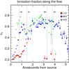 |
Fig. 12 Same as Fig. 11 for xe. |
| In the text | |
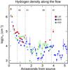 |
Fig. 13 Same as Fig. 11 for log(nH). |
| In the text | |
|
Fig. 14 DG Tau jet width in the first 0.̋7. Each point is the average obtained from four different lines, with the error bars indicating the dispersion. Dashed line: FWHM of the stellar continuum. |
| In the text | |
|
Fig. 15 Mass outflow rate of the jet, Ṁj, using two methods: (i) jet density traversing annuli of nested cones, represented by data points broken down by velocity interval and also totalled; (ii) jet density obtained via emission line luminosities from a uniform slab, as in Hartigan et al. (1995), represented by curves. Uncertainties are about 50% in every velocity interval. |
| In the text | |
|
Fig. 16 1D profile of the [S ii]31/16 ratio along the flow, derived from integration of the line surface brightness across the jet and over each velocity interval. Horizontal dashed lines indicate upper and lower density limits on validity of the ratio as a ne diagnostic. Empty symbols mark positions and velocities for which the modified BE-technique has been applied. Upper and lower limits arise when one of the lines is undetected, and so its flux has been set to 3σ. |
| In the text | |
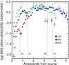 |
Fig. 17 Same as Fig. 16 for the logarithm of the [N ii]/[O i] line ratio. |
| In the text | |
|
Fig. 18 Same as Fig. 16 for the [O i]/[S ii] line ratio. Due to the prominence of [O i] emission over the [S ii] lines close to the star, a few points are off the scale. Their values are: 6.58 at 0.̋175, for the MVI, and 12.10, 14.49, 9.54 and 4.99 at 0.̋175, 0.̋275, 0.̋375 and 0.̋475, respectively, for the HVI. |
| In the text | |
Current usage metrics show cumulative count of Article Views (full-text article views including HTML views, PDF and ePub downloads, according to the available data) and Abstracts Views on Vision4Press platform.
Data correspond to usage on the plateform after 2015. The current usage metrics is available 48-96 hours after online publication and is updated daily on week days.
Initial download of the metrics may take a while.