| Issue |
A&A
Volume 564, April 2014
|
|
|---|---|---|
| Article Number | A75 | |
| Number of page(s) | 7 | |
| Section | Astronomical instrumentation | |
| DOI | https://doi.org/10.1051/0004-6361/201423422 | |
| Published online | 10 April 2014 | |
Cross-calibration of the XMM-Newton EPIC pn and MOS on-axis effective areas using 2XMM sources
1 Dept. of Physics and Astronomy, Leicester University, Leicester LE1 7RH, UK
e-mail: amr30@star.le.ac.uk
2 XMM-Newton Science Operations Centre, ESAC, Apartado 78, 28691 Villanueva de la Cañada, Madrid, Spain
Received: 14 January 2014
Accepted: 13 March 2014
Aims. We aim to examine the relative cross-calibration accuracy of the on-axis effective areas of the XMM-Newton EPIC pn and MOS instruments.
Methods. Spectra from a sample of 46 bright, high-count, non-piled-up, isolated on-axis point sources are stacked together, and model residuals are examined to characterize the EPIC MOS-to-pn inter-calibration.
Results. The MOS1-to-pn and MOS2-to-pn results are broadly very similar. The cameras show the closest agreement below 1 keV, with MOS excesses over pn of 0–2% (MOS1/pn) and 0–3% (MOS2/pn). Above 3 keV, the MOS/pn ratio is consistent with energy-independent (or only mildly increasing) excesses of 7–8% (MOS1/pn) and 5–8% (MOS2/pn). In addition, between 1–2 keV there is a “silicon bump” − an enhancement at a level of 2–4% (MOS1/pn) and 3–5% (MOS2/pn). Tests suggest that the methods employed here are stable and robust.
Conclusions. The results presented here provide the most accurate cross-calibration of the effective areas of the XMM-Newton EPIC pn and MOS instruments to date. They suggest areas of further research where causes of the MOS-to-pn differences might be found, and allow the potential for corrections and possible rectification of the EPIC cameras to be made in the future.
Key words: instrumentation: detectors / instrumentation: miscellaneous / telescopes / X-rays: general
© ESO, 2014
1. Introduction
XMM-Newton (Jansen et al. 2001), a cornerstone mission of ESA’s Horizon 2000 science programme, was designed as an X-ray observatory able to spectroscopically study cosmic X-ray sources with a very large collecting area in the 0.2−10 keV band. This high throughput is achieved primarily through the use of three highly nested Wolter type I imaging telescopes. One of the three co-aligned XMM-Newton X-ray telescopes has an unimpeded light path to the primary focus, where the European Photon Imaging Camera (EPIC) pn camera (Strüder et al. 2001) is positioned. The two other telescopes have EPIC-MOS cameras (Turner et al. 2001) at their primary foci, but receive only approximately half of the incoming radiation, the remainder being diffracted away by Reflection Grating Assemblies (RGAs) towards the secondary foci (where the Reflection Grating Spectrometers (RGS; den Herder et al. 2001) are situated).
The effective area of the EPIC instruments is defined here as the product of the mirror’s effective area, the detector quantum efficiency, and the filter transmission, and is an extremely important quantity to have accurately established. In more detail, further complications can include that the effective area for the MOSs includes the RGA transmission factors, that one cannot extract 100% of the source counts unless one uses unworkably large extraction regions (i.e. point spread function [PSF] concerns), that contamination of the mirror and/or detector may be present, that the full detector efficiency can include other effects in addition to the quantum efficiency such as out-of-time events, and that the mirror’s effective area includes vignetting, which though minimized on-axis, is still important. Furthermore, since the EPIC CCDs are sensitive to IR-UV light, a filter wheel provides a choice of optical blocking filter, including thin, medium, and thick filters (plus open and closed). Use of these filters alters the low-energy X-ray transmission and requires extra specific detailed calibration.
Many attempts have been made to quantify the effective area of the EPIC instruments more and more precisely (and other instruments, both on XMM-Newton and on other X-ray observatories), and this has been one of the main drivers behind IACHEC1− the International Astronomical Consortium for High Energy Calibration, formed to provide standards for high-energy calibration and to study the cross-calibration between different high-energy observatories in detail.
This work describes a new attempt to establish the relative cross-calibration accuracy of the on-axis effective areas of the XMM-Newton EPIC pn and MOS instruments, using a sample of bright, isolated point sources, selected from the 2XMM catalogue. The results provide the most accurate cross-calibration to date of the EPIC pn and MOS effective areas. The structure of the paper is as follows. Section 2 describes the sample selection and analysis. Section 3 describes the results obtained. In Sect. 4 we discuss these results and the further tests that were made, and in Sect. 5 we present our conclusions. Unless otherwise stated, a reference to the term MOS1, MOS2, or pn indicates that particular “whole telescope” system.
2. Analysis
2.1. Sample selection and data reduction
Sources were selected from the entire 2XMM (2XMMi-DR3) catalogue (Watson et al. 2008), as follows. The sources:
-
(i)
are identified within 2XMM as point-like (i.e. no extension),thus maximizing the signal-to-noise ratio, simplifying andunifying the spectral and effective area analysis, and maintainingconsistency of extent across the sample.
-
(ii)
have been observed in full-frame mode alone. This is the most common EPIC observing mode, and it has the most accurate event energy calibration since the CCD charge transfer inefficiency (CTI) models are best derived from full frame data. Full-frame mode has 100% livetime in both pn and MOS, and offers the best background subtraction because of the active silicon relatively near any on-axis source. Mode consistency is maintained across the sample.
-
(iii)
utilize either the thin or medium filter in all of MOS1, MOS2, and pn. These are the two most common EPIC filters employed. Consistency of filter is maintained across the sample.
-
(iv)
have large numbers of (0.2−12 keV) counts (>5000 for MOS1 or MOS2 and >15 000 for pn). Though a larger number of fainter sources could be used in addition to boost the statistics, much more screening would be necessary, and background-modelling and source-to-background effective area issues would become more significant.
-
(v)
have a countrate below the appropriate pile-up limits2 (0.70 ct/s [MOS full-frame], 6 ct/s [pn full-frame]). Pile-up distorts both the spatial and spectral distributions of the photons away from the well-understood non-piled-up case, and thus introduces extra unwanted problems into the analysis. Although the potential “pile-up”-free sample could be increased by using window mode data (with their shorter frame times), only full-frame mode data is used (see above).
-
(vi)
are situated near on-axis, with EP_OFFAX (the smallest value of the MOS1, MOS2 or pn boresight-to-source distances) being <2′. We are concerned here with the effective area cross-calibration on-axis, where all the proposed EPIC source targets are situated, and where the calibration is most mature (also the vignetting is minimized). Later work, outside of the scope of the present paper, hopes to look at the effective area cross-calibration off-axis, where many additional issues come into play; CCD gaps, different CCDs, increased vignetting, elongated PSFs, obscuration by the Reflection Grating Array (RGA) etc.
-
(vii)
lie out of the plane of the Galaxy (|b|>15 deg), where the Galactic column density is generally lower than at low Galactic latitudes. This minimises possible unknown effects due to absorption.
This gave rise to 87 sources. This is a very small number given the number of sources in the 2XMM catalogue (over 350 000), and this is because the above criteria applied are collectively extremely restrictive. For each of these sources, the appropriate raw data – the Observation Data Files (ODFs) – for each source were identified and obtained, and the standard SAS procedures (“epchain” for pn, “emchain” for MOS) were run on these to create the standard calibrated event lists. SAS version v12.0.0 and the then most up-to-date public calibration files, created in late October 2012, have been used throughout the analysis. Calibration is a continually evolving process, and as such this analysis (like all others) provides only a snapshot of the situation at the time of the analysis. It is worth noting that the latest SAS version and calibration files at the time of writing include a correction in the MOS effective area for an evolving contamination layer3. This is modelled as a pure carbon layer on the MOS detector and is relatively thin, having an estimated depth at current epochs in 2013 of only 0.015 μm and 0.04 μm on MOS1 and MOS2 respectively. This is less than 20% of the estimated thickness of the evolving carbon contaminant known to be on the RGS detector. There is no evidence as yet for a contaminant on the pn. As this study deals with sources detected prior to October 2008, the effect of the MOS contaminant model on this study is negligible.
The calibrated event lists were then filtered for periods of high background (solar proton flares) via good time interval (GTI) files. Single pattern lightcurves were created in the 10−15 keV band, with 100 s binning, across the full detectors (excluding MOS1/2 CCD1 and pn CCD4, which contain the sources under study), and then GTIs were then defined as those bins containg less than 130 (pn) or 40 (MOS) counts per bin. A common GTI (combining the MOS1, MOS2, and pn GTI files) was calculated, and this was then used to filter the MOS1, MOS2, and pn event files. Large-scale images around each source were created, and sources were rejected in the following cases; (i) crowded fields, where neighbouring sources lay within the target source region, or where there was no appropriate source-free background region; (ii) when the source had only a very short (<1 ks) common GTI-filtered exposure time; (iii) where chip gaps or bad CCD columns were seen to lie too close to the target source; (iv) where the source appeared to be extended (or to lie within extended emission); (v) there was a loss of an entire detector chip or quadrant. Cases (i) and (ii) accounted for the vast majority of the exclusions, and this yielded a final sample of 46 sources, which are listed in Table 1.
The final sample of 46 EPIC on-axis point sources.
2.2. Data analysis and spectral reduction
For each source and for each instrument, unbinned source spectra were extracted from a complete circle of radius 40′′, centred on the 2XMM source position. A background spectrum was extracted from a complete 90−180′′ annulus, again centred on the 2XMM source position. Cases where the background region appeared contaminated with other sources were removed in the above screening stage, thus keeping both the source (pure circle) and background (pure annulus) extraction regions as clean and as simple as possible. For each source, the three EPIC instruments each cover the same source and background regions on the sky. The estimated source contribution to the background is equally low (<5%) for all three cameras, and this total background only accounts for ≈2% of the extracted total source flux. The spectral extraction criteria that is recommended4 to the general XMM-Newton user were employed: PATTERN no greater than 12 for MOS, no greater than 4 for pn, flag selections of #XMMEA_EM for MOS, and FLAG==0 for pn, and using spectralbinsize=5 in evselect. Standard energy response matrices (RMFs) and effective area files (ARFs) were created for each spectrum via the standard SAS tools.
Then for each instrument, the source spectral counts C were stacked together, using various ftools5 (and exposure-weighting the BACKSCAL values):  where i refers to the ith spectral bin and j refers to the jth source. The background spectral counts B were stacked together in the same manner (exposure-weighting the BACKSCAL values).
  Slightly different source and background BACKSCAL values are seen from source to source within each detector, as different (and time-dependent) bad pixels and columns reduce the “good” detector areas. An average exposure-weighted ARF was calculated, summing the effective areas (EA) in the same way, using ftools:
  An average exposure-weighted RMF was calculated using the ftool addrmf, while ensuring that the sum of the individual exposure-weights was unity. The final output for each instrument (MOS1, MOS2, and pn) is then: one source spectrum, one background spectrum, one ARF and one RMF.
The spectral analysis that follows is confined to energies above 0.5 keV where relative uncertainties in the instruments are dominated by the components of the effective area calibration. At lower energies, the RMF of both pn and MOS becomes strongly non-Gaussian in shape and the interpretation of residuals in the cross-calibration becomes increasingly influenced by uncertainties in the RMF calibration.
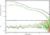 |
Fig. 1 Spectral fitting of the full stacked data from the sample of 46 sources. A phenomenological spectral model is fit closely to the pn data (black points). This model (for details, see text) is then convolved with the instrument responses of MOS1 (red) and MOS2 (green). Data and model are shown in the upper panel, and the residuals are shown in the lower panel. Ratioing the residuals reveals how MOS1 and MOS2 vary with respect to pn. |
2.3. Spectral analysis
To examine the relative cross-calibration accuracy of the effective areas of the EPIC instruments, we applied the method of Longinotti et al. (2008), in a similar manner to that performed in Kettula et al. (2013). This method involves a choice of a reference instrument, against which the other instruments are compared. As it is not known which, if any, of the instruments has a perfectly calibrated effective area, the choice of the reference instrument is arbitrary and the comparison is a relative one. The pn detector was chosen as the reference instrument, reasons being that the more sensitive pn mainly “drives” any all-EPIC fit, and that pn appears to be extremely stable; pn flux measurements below 1 keV are stable within 3% (at the 3σ level) over the whole of XMM-Newton’s operational life (Sartore et al. 2012), though this is probably still a very conservative upper limit (Pollock et al., in prep.), and pn is likely in fact to be much more stable.
How MOS1 and MOS2 vary with respect to pn can then be inspected. This method − firstly stacking all the data together, and then performing spectral fitting on these stacked data − we will later refer to as a “stack and fit” method. For two instruments, here pn and MOS, we begin with the data (data pn,MOS) and the responses (resp pn,MOS), defined here as the energy response matrix (RMF) multiplied by the effective area (ARF) of the instruments. The pn is used as the reference instrument (pn) and spectral analysis is performed on the pn data to fit a reference model (model pn). Several multi-component phenomenological models were constructed to closely fit the pn data to varying degrees of precision. The details of the phenomenological models are actually not important in this study, as usage of models of different complexity − using models of varying “goodness” − essentially produced no changes in the final result, the α ratio (see below). Typically though, the models included some absorption, one or two power laws, a small number of Gaussians, and sometimes an edge. A model that closely fits the pn data is shown (with residuals) in Fig. 1, and is as follows: wabs (nH = 1.84 × 1021 cm-2) × [power (Γ = 4.09) + power (Γ = 1.43) + Gauss (E = 0.59 keV) + Gauss (E = 0.88 keV) + Gauss (E = 5.03 keV) ] × edge (E = 6.85 keV). The reduced chi-squared for this model fit to the pn data is 1.19 for 1888 degrees of freedom.
To compare the two instruments, we ensure that the data (data pn,MOS) are of equal binning. We note here the minor caveat that the binning is in PI space, which may not necessarily correspond to exactly the same photon energy ranges, due to the slightly different redistributions in MOS and pn, however this effect is negligible in our case, as the energy bins of the stacked residual spectra shown in this paper are larger than, or at least comparable to the instrumental energy resolution of the EPIC cameras. We convolve the reference model (model pn) with the instrument responses of MOS1 and MOS2 to produce pn-based model MOS predictions (model MOS | pn). We then divide the MOS data by these model predictions to obtain residuals over the pn-based prediction (resid MOS) The model MOS predictions and residuals are also shown in Fig. 1.
Lastly, to obtain the comparison between MOS and pn, we divide the above residuals of MOS with the pn residuals, to remove effects of possible calibration uncertainties of pn, obtaining a ratio α= resid MOS/ resid pn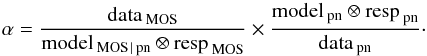 (1)The ratio α is then a useful measure of the effective area cross-calibration, since the value for each energy bin would be unity if the cross-calibration of the pn and MOS effective areas were consistent.
In a more formal analysis, along the lines of e.g. Marshall et al. (2004), we can start from the formal equation for the count spectrum for one source j in the sample for instrument xx (where xx = MOS or pn): 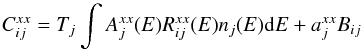 (2)where Tj is the exposure time of the jth source,
  is the effective area for source j for instrument xx, axx refers to the BACKSCAL parameter for source j for instrument xx, Bij is the background count spectrum for source j, nj(E) is the photon spectrum of source j, and
  is the RMF for source j, giving the fraction of events going into instrument xx’s PI bin i that originate at energy E.
The MOS-to-pn ratio of source counts for the stacked spectra is therefore: 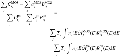 (3)where
  and
and  are the true MOS and pn effective areas.
We can then define a parameter α′ relating the ratio of the effective areas currently assumed to be correct to the true effective areas: 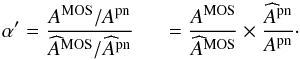 (4)This α′ parameter is equal to the α ratio above in Eq. (1), and we have:
 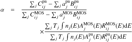 (5)This is true as
  is unity for both the MOS and pn instruments. Also as long as nj(E) and Aj(E) only vary slowly over a spectral channel − this in principle does not hold at energies where the effective area has the steepest gradient, i.e. close to the Si (≃1.8 keV) and Au (≃2.2 keV) edges. This may introduce features in the stacked spectrum. While one indeed sees structures in the residuals of the stacked spectrum against its best-fit model, the amplitude of these features is comparable to that observed when fitting individual spectra. They can be reconnected to imperfect calibration of the MOS Quantum Efficiency, and EPIC effective areas, respectively.
3. Results
Figure 1 shows (by design) a very good fit to the pn data, and a less good fit to the MOS data − the MOS1 and MOS2 data points appear to lie slightly above the model across much of the energy range − this is examined in more detail below. The method described here has removed or minimized as many sources of error or uncertainty as possible. Source variability cannot be the cause of the MOS-to-pn differences, as common GTIs across all the instruments have been used for each of the sources. All the sources are below the pile-up limit in all the instruments, so pile-up is not an issue. Consequently, it has therefore been possible to use a large, full circular region for the spectral extraction, such that any PSF inaccuracies have been minimized (i.e. importantly we have not had to excise any piled-up central core). Furthermore, the problem that all the sources may be spectrally rather different, some having perhaps complex spectra, is overcome by stacking all the spectra together into a single spectrum, and fitting this phenomenologically. We discuss this issue further in Sect. 4.
Once we have the pn, MOS1 and MOS2 residuals, we are then able to ratio these residuals to obtain α, and show how MOS1 and MOS2 vary with respect to pn. This ratio, described above, removes any differences between the pn data and the pn model prediction, and is seen to be insensitive to the general quality of the pn fit (so long that it is adequate − i.e. regardless of the quality of the fit, so long that a by-eye inspection of the residuals indicated that no spectral feature was still unaccounted for, then no change in the residual ratio α is observed). These α ratios for MOS1/pn and for MOS2/pn are shown as the bold points in Fig. 2. Here, adaptive binning of the results has been used to follow the quality of the statistics across the energy range. At low energies (<1 keV), small (0.05 keV) bins have been used, as there are many counts. At high energies (>7 keV), large (1.0 keV) bins have been used, as there are fewer counts.
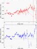 |
Fig. 2 How MOS1 (top panel) and MOS2 (bottom panel) vary with respect to pn. α ratios for MOS1/pn (red) and for MOS2/pn (blue) are plotted against energy (bold points). The data have been adaptively binned to follow the statistics. The faint points, connected by a thin line, show the results obtained using the “fit and stack” (see Sect. 4) analysis (the last MOS2/pn point is at α ≈ 0.75). |
To first order, the MOS1 and MOS2 plots appear very similar. Generally, the MOS/pn α ratio is, at low energy (<1 keV), flat and low (α ≈ 1.00–1.03). This is the energy range over which MOS and pn agree best. Then over the medium energy range, it rises, to flatten out again beyond 3 keV at a higher (close to) energy-independent value (α ≈ 1.05–1.08). On top of this function, where the growth is slowest at the beginning and the end of the function, there is a “bump” at 1−2 keV, which we hereafter call the “silicon bump”, and which may be larger in MOS2 than in MOS1. There are perhaps in addition other small differences between MOS1 and MOS2 that are close in size to the level of the statistical uncertainties; at high energies MOS1/pn may be slightly higher than MOS2/pn, whereas at low energies the reverse may be the case.
4. Discussion
There have been a number of attempts to accurately quantify the effective area – the product of the mirror effective area, the detector quantum efficiency and the filter transmission – not only of the EPIC instruments, but also of other X-ray instruments. The various strategies have certain advantages and disadvantages. Kettula et al. (2013) for instance, studied a sample of clusters of galaxies with the XMM-Newton/EPIC, Chandra/ACIS, BeppoSAX/MECS and Suzaku/XIS instruments. The advantages of using clusters of galaxies is that they are constant and unvarying and they are spectrally quite simple. However clusters are also extended and diffuse and this complicates the analysis, especially with regard to modelling the background and PSF issues. Very bright point sources, e.g. radio loud AGN, have been used for cross-calibration purposes (e.g. Stuhlinger et al. 2010). Here the advantages include the fact that the sources are very bright and, unlike the clusters, point-like. However, these sources are often too bright and consequently suffer from pile-up. Dealing with the pile-up, usually by excising the core of the emission (a non-optimum method given the azimuthal profile of the emission), can introduce errors if the PSF is not extremely accurately calibrated. Also these sources are variable. This problem can be circumvented by defining common GTIs to cover all the instruments in question. In the present paper, we have used various 2XMM point sources that are less bright and are therefore not piled-up. We do not need to excise the core and a full circular extraction region can be used, minimising any PSF issues. Another point is that the selection criteria employed only yielded a few tens of sources from the initial 2XMM catalogue of 350 000. This is an extremely small number, the criteria being extremely restrictive, and indicates why such a study as this has not been possible before now − many years of mission time have been needed in order to accumulate enough suitable sources. These sources may be variable (many of the 46 sources are AGN), but common GTIs have been used to deal with this. One remaining issue with the 2XMM sample is that the sources may be spectrally complex and/or different from one another. We discuss this issue in the following paragraphs.
In the analysis of Kettula et al. (2013), the residuals ratio analysis was performed on each source in their sample separately, and then the median and median absolute deviation of their α values were calculated for each energy channel for their sample. This represents more of a “fit and stack” analysis, as opposed to the “stack and fit” analysis presented in this paper. To test the validity of both methods, a “fit and stack” analysis was performed on our sample of 46 sources. This involved the spectral fitting of each of the 46 pn spectra separately, then convolving each model with the individual MOS instrument responses, to obtain 46 separate residual ratio datasets, from which the median and median absolute deviations could be calculated. These individual spectral fits were performed using χ2 goodness-of-fit tests, after standard spectral grouping using “specgroup”. Only those sources where the reduced χ2 was lower than 1.5 were retained in the final median analysis. We note that likelihood-based tests may have yielded a better agreement.
The results for the “fit and stack” method are shown as the faint points connected by thin lines in Fig. 2. It is seen that the agreement between the “stack and fit” and the “fit and stack” methods on the sample of 46 sources is very good in both MOS1 and MOS2 below 4 keV. Above 7 keV for MOS1, and above 5 keV for MOS2, a deficit in the α ratio is seen for the “fit and stack” method, which is not seen in the “stack and fit” results. Investigating further, we tentatively attribute the deficit to a background subtraction problem involving the error bars on the negative spectral bins that can sometimes occur in the individual source spectra, but not in the (high statistic) stacked spectrum. We conclude that the “stack and fit” method yields consistent results to the “fit and stack” method, and probably gives better results over energy ranges where there are many negative background-subtracted channels (due to statistical fluctuations of the background subtraction). If anything, the “stack and fit” method used here appears to be the more robust of the two.
An important epoch-dependent effect is the low-energy on-axis “patch” in both MOS instruments (Read et al. 2005). Here, the redistribution function is seen to evolve with time such that an increasing fraction of X-rays suffer incomplete charge collection. The effect is increasingly stronger towards lower energies, and appears to be related to the total X-ray radiation dose received by a pixel which will clearly be higher at the centre of the detector. Sources at MOS off-axis angles greater than 2′ are essentially immune to this effect. For MOS on-axis sources, photons from the energy band 0.2–0.5 keV can be redistributed in energy below the detection threshold and lost, while photons from energy band 0.5–1.0 keV can be redistributed into the 0.2–0.5 keV energy band. The effect is negligible at energies above 1 keV. The “patch effect” has been extensively studied, and is well calibrated. All but 4 of the 46 sources are seen to lie on the MOS patch. As a sanity check, we looked at the results obtained with the full stacked data, but using single RMFs from the beginning, the middle, and the end of the mission time period considered (revolutions <1800). The only effects seen were (as expected) those at low-energy due to the evolving patch and were entirely consistent with the known (and calibrated) instrumental evolution. Usage of the beginning (end) RMF introduces a downwards (upwards) offset of 5% in the α ratio at 0.5 keV, for both MOS1/pn and MOS2/pn, when compared with using the correct exposure-weighted average of the RMFs. This offset decreases to zero at 1.3 keV and remains at zero out to 10 keV. The “stacked” RMF that we have employed, an exposure-weighted average of the RMFs constructed for each separate source, is seen to behave entirely correctly, and as expected when compared with the single RMF cases and factoring in the epoch- and exposure-distrutions of the contributing files.
It is hard to resolve the cross-calibration discrepancies between the EPIC cameras reported here just by changing the quantum efficiency calibration, without violating the ground-based measurements (see Turner et al. 2001; Saxton & Sembay 2004). However, the overall shape of the stacked residuals indicates that a change in the quantum efficiency could contribute to alleviating the problem. A change in the energy-dependent quantum efficiency of the MOS detectors, say, which has an intrinsically larger silicon edge than the pn, could remove at least part of the “silicon bump” and part of the “slow-faster-slow” energy-dependence of the MOS/pn beaviour. Furthermore, a mis-calibration of the silicon fluorescence peak may be a cause of part of the “silicon bump”. Further analysis may help in understanding which other calibration element(s) might be involved, and might require further detailed investigation.
5. Conclusions
We have examined the accuracy of the relative cross-calibration of the on-axis effective areas of the XMM-Newton EPIC pn and MOS instruments. A sample of 46 bright, high-count, non-piled-up, isolated, on-axis point sources was selected from the 2XMM catalogue. After flare- and background-cleaning, and applying common GTI filtering, source and background spectra extracted from the 46 sources were stacked together, and the individual response files were averaged in an exposure-weighted manner. Spectral fitting was applied, and the MOS and pn model residuals were examined in order to characterize the EPIC MOS-to-pn inter-calibration. It was seen that the MOS1-to-pn and MOS2-to-pn results are broadly very similar, with the cameras showing the closest agreement below 1 keV, with MOS excesses over pn of 0–2% (MOS1/pn) and 0–3% (MOS2/pn). Above 3 keV, the MOS/pn ratio is consistent with an energy-independent (or only mildly increasing) ratio, with MOS excesses of 7–8% (MOS1/pn) and 5–8% (MOS2/pn). In addition to this, between 1–2 keV there is a further excess − a “silicon bump” − at a level of 2–4% (MOS1/pn) and 3–5% (MOS2/pn). Tests reveal that the “stack and fit” methods employed here appear to be stable and robust, and the results presented here provide the most accurate to date cross-calibration of the on-axis effective areas of the XMM-Newton EPIC pn and MOS instruments. Areas of research where possible causes of the MOS-to-pn mismatches might be found are suggested by the analysis, and we note the potential for future corrections to and possible rectification of the EPIC MOS and pn cameras to be made.
XMM-Newton Users Handbook (v.2.10): http://xmm.esac.esa.int/external/xmm_user_support/documentation/uhb/XMM_UHB.html
Acknowledgments
The XMM-Newton project is an ESA Science Mission with instruments and contributions directly funded by ESA Member States and the USA (NASA). We thank members of the EPIC cross-calibration working group − Jukka Nevalainen, Martin Stuhlinger, Frank Haberl, Silvano Molendi, Richard Saxton and Michael Smith − for helpful discussions. We also thank the referee Herman Marshall for very useful comments and discussions which have improved the paper. A.M.R. and S.S. acknowledge the support of STFC/UKSA/ESA funding.
References
- den Herder, J. W., Brinkman, A. C., Kahn, S. M., et al. 2001, A&A, 365, L7 [NASA ADS] [CrossRef] [EDP Sciences] [Google Scholar]
- Jansen, F., Lumb, D., Altieri, B., et al. 2001, A&A, 365, L1 [NASA ADS] [CrossRef] [EDP Sciences] [Google Scholar]
- Kettula, K., Nevalainen, J., & Miller, E. D. 2013, A&A, 552, 47 [Google Scholar]
- Longinotti, A. L., de La Calle, I., Bianchi, S., Guainazzi, M., & Dovciak, M. 2008, Rev. Mex. Astron. Astrofis. Conf. Ser., 32, 62 [NASA ADS] [Google Scholar]
- Marshall, H. L., Dewey, D., & Ishibashi, K. 2004, In-Flight Calibration of the Chandra High Energy Transmission Grating Spectrometer, Proc. SPIE, 5165, 457 [NASA ADS] [CrossRef] [Google Scholar]
- Read, A. M., Sembay, S. F., Abbey, T. F., & Turner, M. J. L. 2006, Proc. X-ray Universe 2005, 26–30 September 2005, El Escorial, Madrid, Spain, ed. A. Wilson, ESA SP, 604, 925 [Google Scholar]
- Sartore, N., Tiengo, A., Mereghetti, S., et al. 2012, A&A, 541, 66 [Google Scholar]
- Saxton, R. D., & Sembay, S. 2004, EPIC MOS low energy response and Quantum Efficiency, http://xmm2.esac.esa.int/docs/documents/CAL-SRN-0169-1-1.ps.gz [Google Scholar]
- Stuhlinger, M., et al. 2010, Status of XMM-Newton Instrument Cross-Calibration with SASv10.0, http://xmm2.esac.esa.int/docs/documents/CAL-TN-0052.ps.gz [Google Scholar]
- Strüder, L., Briel, U., Dennerl, K., et al. 2001, A&A, 365, L18 [NASA ADS] [CrossRef] [EDP Sciences] [Google Scholar]
- Turner, M. J. L., Abbey, A., Arnaud, M., et al. 2001, A&A, 365, L27 [NASA ADS] [CrossRef] [EDP Sciences] [Google Scholar]
- Watson, M. G., Schröder, A. C., Fyfe, D., et al. 2009, A&A, 493, 339 [NASA ADS] [CrossRef] [EDP Sciences] [Google Scholar]
All Tables
All Figures
|
Fig. 1 Spectral fitting of the full stacked data from the sample of 46 sources. A phenomenological spectral model is fit closely to the pn data (black points). This model (for details, see text) is then convolved with the instrument responses of MOS1 (red) and MOS2 (green). Data and model are shown in the upper panel, and the residuals are shown in the lower panel. Ratioing the residuals reveals how MOS1 and MOS2 vary with respect to pn. |
| In the text | |
|
Fig. 2 How MOS1 (top panel) and MOS2 (bottom panel) vary with respect to pn. α ratios for MOS1/pn (red) and for MOS2/pn (blue) are plotted against energy (bold points). The data have been adaptively binned to follow the statistics. The faint points, connected by a thin line, show the results obtained using the “fit and stack” (see Sect. 4) analysis (the last MOS2/pn point is at α ≈ 0.75). |
| In the text | |
Current usage metrics show cumulative count of Article Views (full-text article views including HTML views, PDF and ePub downloads, according to the available data) and Abstracts Views on Vision4Press platform.
Data correspond to usage on the plateform after 2015. The current usage metrics is available 48-96 hours after online publication and is updated daily on week days.
Initial download of the metrics may take a while.