| Issue |
A&A
Volume 564, April 2014
|
|
|---|---|---|
| Article Number | A128 | |
| Number of page(s) | 18 | |
| Section | Extragalactic astronomy | |
| DOI | https://doi.org/10.1051/0004-6361/201323123 | |
| Published online | 17 April 2014 | |
Fueling the central engine of radio galaxies
III. Molecular gas and star formation efficiency of 3C 293⋆,⋆⋆
1 Centro de Astrobiología (CSIC-INTA), Carretera de Ajalvir km. 4, 28850 Torrejón de Ardoz, Madrid, Spain
e-mail: This email address is being protected from spambots. You need JavaScript enabled to view it.
2 Observatorio Astronómico Nacional, Alfonso XII 3, 28014 Madrid, Spain
3 Observatoire de Paris, LERMA & CNRS UMR 8112, 61 Av. de l’Observatoire, 75014 Paris, France
4 INAF/Osservatorio Astrofisico di Arcetri, Largo Enrico Fermi 5, 50125 Florence, Italy
5 IRAM, 300 rue de la Piscine, Domaine Universitaire, 38406 Saint Martin d’ Hères Cedex, France
Received: 25 November 2013
Accepted: 13 February 2014
Abstract
Context. Powerful radio galaxies show evidence of ongoing active galactic nuclei (AGN) feedback, mainly in the form of fast, massive outflows. But it is not clear how these outflows affect the star formation of their hosts.
Aims. We investigate the different manifestations of AGN feedback in the evolved, powerful radio source 3C 293 and their impact on the molecular gas of its host galaxy, which harbors young star-forming regions and fast outflows of H i and ionized gas.
Methods. We study the distribution and kinematics of the molecular gas of 3C 293 using high spatial resolution observations of the 12CO(1-0) and 12CO(2-1) lines, and the 3 mm and 1 continuum taken with the IRAM Plateau de Bure interferometer. We mapped the molecular gas of 3C 293 and compared it with the dust and star-formation images of the host. We searched for signatures of outflow motions in the CO kinematics, and re-examined the evidence of outflowing gas in the H i spectra. We also derived the star formation rate (SFR) and star formation efficiency (SFE) of the host with all available SFR tracers from the literature, and compared them with the SFE of young and evolved radio galaxies and normal star-forming galaxies.
Results. The 12CO(1-0) emission line shows that the molecular gas in 3C 293 is distributed along a massive (M(H2) ~ 2.2 × 10¹⁰M⊙) ~24″(21 kpc-) diameter warped disk, that rotates around the AGN. Our data show that the dust and the star formation are clearly associated with the CO disk. The 12CO(2-1) emission is located in the inner 7 kpc (diameter) region around the AGN, coincident with the inner part of the 12CO(1-0) disk. Both the 12CO(1-0) and 12CO(2-1) spectra reveal the presence of an absorber against the central regions of 3C 293 that is associated with the disk. We do not detect any fast (≳500 km s-1) outflow motions in the cold molecular gas. The host of 3C 293 shows an SFE consistent with the Kennicutt-Schmidt law of normal galaxies and young radio galaxies, and it is 10–50 times higher than the SFE estimated with the 7.7 μm PAH emission of evolved radio galaxies. Our results suggest that the apparently low SFE of evolved radio galaxies may be caused by an underestimation of the SFR and/or an overestimation of the molecular gas densities in these sources.
Conclusions. The molecular gas of 3C 293, while not incompatible with a mild AGN-triggered flow, does not reach the high velocities (≳500 km s-1) observed in the H i spectrum. We find no signatures of AGN feedback in the molecular gas of 3C 293.
Key words: galaxies: individual: 3C 293 / galaxies: ISM / galaxies: kinematics and dynamics / galaxies: active / ISM: jets and outflows / galaxies: star formation
Based on observations carried out with the IRAM Plateau de Bure Interferometer. IRAM is supported by INSU/CNRS (France), MPG (Germany) and IGN (Spain).
Calibrated data as FITS files are available at the CDS via anonymous ftp to cdsarc.u-strasbg.fr (130.79.128.5) or via http://cdsarc.u-strasbg.fr/viz-bin/qcat?J/A+A/564/A128
© ESO, 2014
1. Introduction
An active galactic nucleus (AGN) releases vast amounts of energy into the interstellar medium (ISM) of its host galaxy. This energy transfer, known as AGN feedback, may increase the temperature of the ISM gas, preventing its collapse, and/or expel it in the form of outflows (see Fabian 2012, for a review). Both effects will inhibit the star formation of the host and affect its evolution. Observational evidence of the effects of AGN feedback on the hosts is frequently found in the literature (Thomas et al. 2005; Murray et al. 2005; Schawinski et al. 2006; Müller Sánchez et al. 2006; Feruglio et al. 2010; Crenshaw et al. 2010; Fischer et al. 2011; Villar-Martín et al. 2011; Dasyra & Combes 2011; Sturm et al. 2011; Maiolino et al. 2012; Aalto et al. 2012; Walter et al. 2013; Silk 2013). It is thought that AGN feedback might be responsible for several properties observed in galaxies, such as the correlations between black hole and host galaxy bulge mass (Magorrian et al. 1998; Tremaine et al. 2002; Marconi & Hunt 2003; Häring & Rix 2004), or the fast transition of early-type galaxies from the blue cloud to the red sequence (Schawinski et al. 2007; Kaviraj et al. 2011). Hence, it is now clear that models of galaxy evolution need to consider the effects of AGN feedback in the host galaxy (King 2003; Granato et al. 2004; Di Matteo et al. 2005; Croton et al. 2006; Ciotti & Ostriker 2007; Menci et al. 2008; King et al. 2008; Merloni & Heinz 2008; Narayanan et al. 2008; Silk & Nusser 2010).
The AGN feedback may take place through two mechanisms: through AGN radiation (known as radiative or quasar mode of AGN feedback), or through interaction of the jet with the ISM (known as kinetic or radio mode). The most intense effects of the kinetic mode are seen in powerful radio galaxies. The extremely large and fast jets of powerful radio galaxies are able to inject enormous amounts of energy into their host galaxy ISM and even into the intergalactic medium (IGM; e.g., Bîrzan et al. 2004; Fabian et al. 2006; McNamara & Nulsen 2007; McNamara et al. 2013; Russell et al. 2014). Most massive galaxies will harbor a radio galaxy phase during their lifetime (e.g., Best et al. 2006). Studying AGN feedback during this phase is thus crucial for understanding galaxy evolution.
A large number of radio galaxies show manifestations of ongoing AGN feedback at different redshift ranges, whether as gas outflows or as inhibition of star formation. Outflows in radio galaxies have been detected through H i and ionized gas observations (e.g., Morganti et al. 2003a; Rupke et al. 2005; Holt et al. 2006; Nesvadba et al. 2006, 2008; Lehnert et al. 2011). Searches for molecular gas, which may dominate the mass/energy budget of the wind, show evidence of outflows only in one radio source (4C 12.50; Dasyra & Combes 2011). Based on the molecular gas contents, and star formation rate (SFR) estimations using the 7.7 μm polycyclic aromatic hydrocarbons (PAH) emission, Nesvadba et al. (2010) found that radio galaxies can be ~10–50 times less efficient in forming stars than galaxies that follow the canonical Kennicutt-Schmidt (KS, Schmidt 1959; Kennicutt 1998b) relationship. The warm-H2 emission of these radio galaxies suggests shocks in the ISM that are induced by the expansion of the powerful radio jet. These shocks are thought to increase the turbulence in the molecular gas, which inhibits the star formation in the host galaxy. However, it is not clear how jet-induced shocks affect the cold phase of the molecular gas.
Our recent work on 3C 236 (Labiano et al. 2013) found that not all radio galaxies show a low star formation efficiency (SFE). 3C 236 is a re-activated radio source that shows an SFE consistent with the KS-law. The young age of its second period of radio-source activity (105 yr, based on the dynamics of the source, Tremblay et al. 2010; O’Dea et al. 2001), and the older age of the Nesvadba et al. (2010) radio source sample (107−108 yr) suggested that the impact of the AGN feedback on the SFR probably evolves with time. A literature search showed that different authors had measured the SFR and M(H2) of the young sources: 4C 12.50, 4C 31.04 (García-Burillo et al. 2007; Willett et al. 2010; Dasyra & Combes 2012). These two sources show an SFE consistent with the KS-law, which supports the evolutionary scenario of the feedback impact. Observations of cold molecular gas in the ISM of different populations of young and evolved radio galaxies and accurate measurements of their SFR are the key to understanding how AGN feedback affects the properties of their hosts.
1.1. 3C 293
The radio source 3C 293 is a large (~200 kpc), powerful (P5 GHz = 9 × 1024 W Hz-1), FR II1 (Fanaroff & Riley 1974) radio galaxy with PA = 135°. The inner 2″ of the radio source show a compact core and two jets aligned east-west (PA = 93°), with the eastern jet approaching. Estimations based on spectral aging show that the large radio source was triggered ≲20 Myr ago and stopped ~0.35 Myr ago, while the compact source was triggered ≲0.18 Myr ago (Akujor et al. 1996; Joshi et al. 2011). The time-lapse between the two activity epochs probably lasted only ≲0.1 Myr (Joshi et al. 2011). This short pause in activity implies that the radio jets of 3C 293 may have been almost continuously interacting with the ISM of the host for the last ~20 Myr.
The host galaxy of 3C 293 (UGC 8782 or VV5-33-12, z = 0.0450, de Vaucouleurs et al. 1991) has been classified both as a spiral galaxy (e.g., Sandage 1966; Colla et al. 1975; Burbidge & Crowne 1979) and as an elliptical galaxy (e.g., Véron-Cetty & Véron 2001; Tremblay et al. 2007), probably because of its extremely complex morphology, with a dust disk, compact knots, and large dust lanes2. The morphology and the vast amounts of gas and dust found in the host of 3C 293 are consistent with a gas-rich merger of an elliptical galaxy with a spiral galaxy (Martel et al. 1999; de Koff et al. 2000; Capetti et al. 2000; Floyd et al. 2006). UGC 8782 shows an optical emission tail that extends beyond a possible companion ~37″ to the southwest (Heckman et al. 1986; Smith & Heckman 1989). It is not clear whether this companion galaxy is interacting with UGC 8782 or was formed in the dust tail (Floyd et al. 2006).
Hubble Space Telescope (HST) near-UV (NUV) photometry of UGC 8782 revealed several regions of bright emission along the edges of the dust lanes, consistent with recent star formation (Allen et al. 2008; Baldi & Capetti 2008). Optical spectroscopy shows that the total stellar mass of 3C 293 is 2.8 × 10¹¹M⊙, consisting of a young (0.1–2.5 Gyr) stellar population, which represents 57% of the total stellar mass, and an old stellar population (≳10 Gyr, Tadhunter et al. 2005). The age of the young stellar population is consistent with a star formation episode after the merger (Tadhunter et al. 2005, 2011). The Starlight (Cid Fernandes et al. 2005) fit of the SDSS spectrum Ca H+K lines showed that the stellar population of 3C 293 can be described by three components with ages 10 Gyr, 0.1–1 Gyr, and 10 Myr (Nesvadba et al. 2010).
The H i spectrum of 3C 293 shows a broad (~1200 km s-1) absorption component associated with the western jet of the compact radio source (0.5 kpc west of the nucleus). This absorption is created in an outflow of neutral gas produced by the interaction of the radio jet with the ISM (Morganti et al. 2003b, 2005; Mahony et al. 2013). Optical, long-slit spectra show an outflowing component in the ionized gas emission lines, with a width and center consistent with those of the H i outflow. This ionized gas outflow, however, is associated with the east component of the compact radio source (1 kpc east of the nucleus). Weaker hints of outflowing ionized gas might also be present in the center and western components of the compact radio source (Emonts et al. 2005).
Based on CO observations made with the NRAO-12 m telescope and the OVRO Millimeter Array, Evans et al. (1999) reported the detection of the 12CO(1-0) line, both in emission and absorption, in 3C 293 (see also Evans et al. 2005). According to their data, which have a spatial resolution of ~3.5″, the 12CO(1-0) emission extends across a 7″ diameter disk, with a total mass of cold H2 of M(H2) ~ 1.5 × 10¹⁰M⊙, and is perpendicular to the large-scale radio source. Later observations, using the JCMT, detected high-excitation CO emission lines in 3C 293 (CO(4-3), CO(6-5), Papadopoulos et al. 2008, 2010). The Plateau de Bure Interferometer (PdBI) was also used to probe the molecular gas using the 12CO(2-1) line, and search for evidence of outflow (García-Burillo et al. 2009). None of the observations above had the required velocity coverage and sensitivity to detect the outflow seen in H i and ionized gas, however.
 |
Fig. 1 Continuum maps of 3C 293 at 3 mm (left) and 1 mm (right). The positions of the AGN and jet components, based on the UV-FIT results (Table 1), are identified with crosses (+). The dashed box marks the size of the 1 mm map shown in the right panel. The contour levels are –9, 9, 39 to 249 mJy beam-1, in steps of 30 mJy beam-1 for the 3 mm map; and –6, 6, 12 to 60 mJy beam-1, in steps of 6 mJy beam-1 for the 1 mm map. (Δ α, Δ δ) = (0,0) corresponds to the position of the AGN at 1 mm. The gray ellipses in the top-right corner show the PdBI beam for each map. |
Even though 3C 293 has large contents of molecular gas and young stars, Nesvadba et al. (2010) measured an SFE 20 times lower than expected for normal star-forming galaxies, based on its 7.7 μm PAH emission and the H2 measurements of Evans et al. (1999). They attributed this low SFE to the impact of AGN feedback on the ISM through the outflows observed in H i and ionized gas. On the other hand, the far-infrared luminosity of 3C 293 (3.3 × 10¹⁰ L⊙, Floyd et al. 2006) is consistent with far-infrared luminosities of normal, KS-law, star-forming galaxies with similar molecular gas contents, suggesting that the SFR of 3C 293 calculated with the 7.7 μm PAH emission may be underestimated.
The large molecular gas content of the host, the ages of the old radio source and young stellar population, the re-ignition of the nuclear activity, and gas outflows caused by jet-ISM interactions make 3C 293 an ideal candidate for studying the impact of AGN feedback in radio galaxies. We carried out 1 mm, 3 mm continuum and 12CO(1-0), 12CO(2-1) line observations of 3C 293 with the PdBI to investigate the impact of AGN feedback of activity in its host. Our sensitivity and resolution at 3 mm are, respectively, five and two times better than achieved before (e.g., Evans et al. 1999), and we covered a velocity range broad enough (>4000 km s-1) to detect the molecular gas counterpart of the H i and ionized gas outflows. In this paper, we present the results of these observations where we study the continuum emission of 3C 293, and analyze the morphology and kinematics of the molecular gas. We determine the systemic velocity of 3C 293, search for outflow signatures in the cold molecular gas, and compare our results with the H i observations of the outflow. We then reassess the SFR of 3C 293 based on several SFR tracers, taking care to examine possible effects of the AGN. Finally, we compare the SFE of 3C 293 with a sample of powerful radio galaxies and normal star-forming galaxies and examine the possible impact of AGN feedback on star formation.
2. Observations
2.1. Interferometer observations
We observed 3C 293 in the 12CO(1-0) and 12CO(2-1) lines, at 3 and 1 mm using six antennas in the D and B configurations, respectively, of the IRAM PdBI (Guilloteau et al. 1992) in January 2011. The receivers were tuned based on the redshift z = 0.0446 (ν0 = 13 371 km s-1), so that the 12CO(1-0) and 12CO(2-1) lines were centered on 110.350 and 220.695 GHz, respectively. With this setting we obtained a velocity coverage of ~10 000 km s-1 at 110.350 GHz and 5000 km s-1 at 220.695 GHz, with the WideX wide-band correlator of the PdBI (3.6 GHz-wide) and the two polarizations of the receiver. Observations were conducted in a single pointing of FWHM ~ 45″ at 110.350 GHz and ~23″ at 220.695 GHz. The adopted phase-tracking center of the observations was set at (α2000, δ2000) = (13h52m17.8s, 31°26′46.2″), the position of the nucleus given by the NASA/IPAC Extragalactic Database (NED). Nevertheless, the position of the AGN determined in Sect. 3, which coincides with the position of the radio continuum VLBI core (Beswick et al. 2004), is ≃0.3″ offset to the north with respect to the array center: (Δ α, Δ δ) ~ (0.0″, 0.3″). Hereafter, all positions are given with respect to the coordinates of the AGN. Visibilities were obtained through on-source integration times of 22.5 min framed by short (2.25 min) phase and amplitude calibrations on the nearby quasar 1308+326. The visibilities were calibrated using the antenna-based scheme. The absolute flux density scale was calibrated on MWC349 and found to be accurate to ≲10% at 220.695 GHz.
The image reconstruction was made with the standard IRAM/GILDAS software (Guilloteau & Lucas 2000)3. We obtained the maps of the continuum emission averaging channels free of line emission from ν− νo = −1810 to –3114 km s-1 for 110.350 GHz, and ν− νo = −1758 to –3035 km s-1 for 220.695 GHz. The corresponding 1σ sensitivities of the continuum emission are ~0.4 mJy beam-1 at 110.350 GHz, and ~0.7 mJy beam-1 at 220.695 GHz. We used natural weighting and no taper to generate the CO line maps, with a field-of-view (FoV) of 51″ and 0.2″/pixel sampling and a synthesized beam of 2.4″× 2.8″ @ PA = 42° at 3 mm, and a FoV of 26″ with 0.1″/pixel sampling, and a synthesized beam of 0.44″× 0.61″ @ PA = 44° at 1 mm. The continuum levels were subtracted in the visibilities plane to generate the line maps. The 1σ point source sensitivities were derived from emission-free channels resulting in 0.9 mJy beam-1 in 5.9 MHz (~16 km s-1)-wide channels for 110.350 GHz, and 1.7 mJy beam-1 in 5.9 MHz (~8 km s-1)-wide channels for 220.695 GHz.
2.2. Supplementary data
We used the following data from the HST archive: STIS/NUV-MAMA/F25SRF2 (hereafter NUV image, Allen et al. 2002; Floyd et al. 2006), WFPC2/F702W (R-band image, Martel et al. 1999; de Koff et al. 2000; Floyd et al. 2006), NICMOS2/F160W (H-band), F170M, F181M and R − H map from Floyd et al. (2006); H i data by Morganti et al. (2003b); mid-IR data from Dasyra & Combes (2011) and Guillard et al. (2012), and the Spitzer archive; Sloan Digital Sky Survey (SDSS) spectra from York et al. (2000), Abazajian et al. (2009), and Buttiglione et al. (2009); William Herschel Telescope (WHT) data from Emonts et al. (2005).
We use H0 = 71, ΩM = 0.27, and ΩΛ = 0.73 (Spergel et al. 2003, 2007) throughout the paper. Luminosity and angular distances are DL = 196.9 Mpc and DA = 180.3 Mpc; the latter gives 1″ = 0.874 kpc (Wright 2006).
 |
Fig. 2 12CO(1-0) and 12CO(2-1) intensity maps of 3C 293, integrating all emission above 3σ levels, from v − vo = −380 to +500 km s-1 and v − vo = −280 to +450 km s-1 respectively. Crosses (+) mark the position of the AGN and jet peak emission according to the UV-FIT models (Table 1). The dashed box in the 12CO(1-0) map marks the size of the 12CO(2-1) map shown in the right panel. Color scales are in Jy beam -1 km s-1. The maps were clipped at 3σ, with σ = 0.11 and 0.13 Jy beam-1 km s-1 for the 12CO(1-0) and 12CO(2-1) maps, respectively. The bottom panels show an overlay of the 12CO(1-0) (color scale) and 12CO(2-1) (contours) emission above 3σ levels. The contour levels are 0.39 to 3.9 Jy beam-1 km s-1, in steps of 0.39 Jy beam-1 km s-1. |
3. Continuum maps
Figure 1 shows the 1 mm and 3 mm continuum maps of 3C 293. The continuum emission at both wavelengths consists of a bright central component plus a fainter one ~1 3 to the east. Using the UV-FIT task of GILDAS, we fitted two point sources to the 1 mm and 3 mm continuum visibilities of 3C 293 (FWHM1 mm ≃ 0.52″, FWHM3 mm = 2.6″). The results of the best fits are given in Table 1. The central component, located at (Δα,
  0, 00), is responsible for 86% and 72% of the emission at 1 mm and 3 mm, respectively. The global-VLBI and MERLIN 1.35 and 1.5 GHz maps show that this central component corresponds to the position of the AGN (component “Core” in Beswick et al. 2004; Floyd et al. 2006). Therefore, we adopted this component as the AGN position of 3C 293 (component labeled “AGN” in Fig. 1).
AGN and jet position.
The eastern component was fitted at both wavelengths by a point source with coordinates (Δα,  3 ± 0.1, +00 ± 01), consistent with the jet component E1 of the global-VLBI and MERLIN 1.35 and 1.5 GHz maps (Beswick et al. 2004; Floyd et al. 2006). The coordinates of the fitted AGN and jet components yield a PA of 89° for the mm-jet(s), consistent with the orientation of the small radio jet determined in the VLBI cm-maps of the source. Therefore, we have detected the mm-counterparts of the approaching jet of the compact radio source of 3C 293 (component labeled “jet” in Fig. 1).
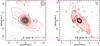 |
Fig. 3 Overlay of the continuum (black) and CO emission (red) emission of 3C 293. Crosses (+) mark the position of the AGN and jet peak emission according to the UV-FIT models (Table 1). The contour levels are 0.33 to 10.23 Jy beam-1 km s-1, in steps of 1.65 Jy beam-1 km s-1 for the 12CO(1-0) map; and 0.39 to 3.9 Jy beam-1 km s-1, in steps of 0.39 Jy beam-1 km s-1 for the 12CO(2-1) map. The contour levels of the continuum are the same as in Fig. 1. |
 |
Fig. 4 R-band (Martel et al. 1999), H-band (Floyd et al. 2006), and R–H (Floyd et al. 2006) images of 3C 293, with the 12CO(1-0) and 12CO(2-1) emissions overlaid. (Δα, Δδ)-offsets in arcsec are relative to the location of the AGN. Crosses (+) mark the position of the AGN and jet peak emission according to the UV-FIT models (Table 1). Solid lines mark the location of the IR counterparts of the Eastern radio lobe (Floyd et al. 2006). The dashed box in the 12CO(1-0) maps mark the size of the 12CO(2-1) maps shown in the right panel. Contour levels as in Fig. 3. |
Using the fluxes of the fitted mm components and the radio emission of 3C 293 between 10 MHz and 10 GHz (available in NED), we searched for the possible origin of the mm emission of 3C 293. The 10 MHz to 10 GHz emission of 3C 293 follows a power law with spectral index ≃− 0.65 ± 0.1. When the total fluxes (AGN plus jet) at 1 mm and 3 mm are added to the data, the spectral index (− 0.62 ± 0.1) is still consistent with synchrotron emission. The 1 mm and 3 mm fluxes of the AGN and jet components, considered separately, are also consistent with synchrotron emission and with the results of Floyd et al. (2006), who showed that the emission from the jet was caused by synchrotron radiation even at near-infrared wavelengths.
4. CO maps
4.1. Distribution of the molecular gas
We mapped the 12CO(1-0) and 12CO(2-1) emission of 3C 293 with spatial resolutions of 2.4″× 2.8″ and 0.44″× 0.61″, respectively. According to our data, 3C 293 shows 12CO(1-0) and 12CO(2-1) emission above significant (>3σ) levels from v − vo = −380 to +500 km s-1, and v − vo = −280 to +450 km s-1, respectively. Figure 2 shows the integrated 12CO(1-0) and 12CO(2-1) emission maps within these velocity ranges. The 12CO(1-0) emission extends to radius~12″ (~10.5 kpc) from the AGN, while the 12CO(2-1) emission extends to radius ~4″ (~3.5 kpc). Even though the 12CO(1-0) emission suggests a smooth morphology, the higher resolution 12CO(2-1) map shows a highly structured CO disk, with knots of emission and absorption regions near the center. Figure 2 shows that the distribution of 12CO(1-0) in 3C 293 is consistent with an elongated disk-like source, with a change in position angle (PA) at radius ~7″: PAmorph ~ 40° for the inner region, PAmorph ~ 55° for the outer region, suggesting a slightly warped molecular gas distribution. The possible presence of a warp is studied in detail in Sect. 4.4 along with the kinematics of the CO gas.The higher resolution 12CO(2-1) map shows that the PAmorph in the inner ≲3″ radius is 55°, and changes to ~40° at radii ~3–4″. This abrupt change in orientation suggests a ridge in the CO disk. Inspection of the 12CO(1-0)–12CO(2-1) overlay (bottom panels of Fig. 2) suggests that the size of the beam might have hidden the ridge in the 12CO(1-0) map.
Evans et al. (1999) observed that the 12CO(1-0) emission in 3C 293 was produced by a 7″ (6 kpc) diameter disk around the core of 3C 293 (see also Evans et al. 2005). The large difference between their measurements and our observations is due to the better sensitivity and resolution of the PdBI 12CO(1-0) data. Using single-dish, JCMT spectra, Papadopoulos et al. (2008) measured ~3 times more 12CO(2-1) flux in 3C 293 than we see in our 12CO(2-1) map, which suggests that the difference in the extension of the 12CO(1-0) emission (below 3σ at radius ~12″) and 12CO(2-1) emission (below 3σ at radius ~4″) in our data might be due to the sensitivity and PdBI filtering of the 12CO(2-1) emission on large scales. With the B-configuration, we loose flux at distances ≳4″ at 1 mm.
Papadopoulos et al. (2010) measured extremely high ratios for the CO lines: CO(6-5)/CO(3-2) and CO(4-3)/CO(3-2) in 3C 293 (R65/32 = 1.3 ± 0.54, R43/32 = 2.3 ± 0.91). Figure 3 shows the superposition of the mm continuum and CO emission maps. The 12CO(2-1) map shows a region in front of the 1 mm core without CO emission, suggesting a CO absorber against the core. The 12CO(1-0) map shows fainter emission towards the center, consistent with an absorber, although the flux variations are weaker than the 12CO(2-1) map because of the larger size of the 12CO(1-0) beam. Our data suggest that the high line ratios measured by Papadopoulos et al. (2010) might be caused by the CO absorber towards the central regions of 3C 293, because lines with low-J values are more affected by absorption than the high-J lines, which in turn yields overestimated ratios.
Figure 4 shows the 12CO(1-0) and 12CO(2-1) maps superposed on the HST R-band, H-band, and R − H color images of 3C 293. The R-band image shows two optical absorption systems: a disk-like dust structure in the inner ≲1 kpc radius, and the large-scale (≳10 kpc radius) tidal features responsible for the dust lanes that criss-cross the galaxy in front of the nucleus (Heckman et al. 1986; Smith & Heckman 1989; Evans et al. 1999; Floyd et al. 2006). The dust disk is oriented along the northwestern edge (where obscuration is higher) towards us. The H-band image shows that the IR counterparts of the Eastern jet radio lobe, which are on the approaching side of the radio source, are emerging from the southeastern side of the disk (Floyd et al. 2006). gions 1 The overlays of the CO emission and the R, H, and R − H maps show that the 12CO(2-1) emission follows the edge of the dust disk in the northwest, suggesting that the molecular gas is associated with the dust disk. The R − H map shows that the extinction follows the 12CO(1-0) emission contours up to distances of at least ~12″ (radius). Furthermore, the extinction in 3C 293 also follows the warped structure of the CO disk, supporting that the dust and CO disk are associated up to distances ≳12″ (10.5 kpc). Hence, our observations suggest that 3C 293 hosts a warped molecular gas (and dust) disk that extends at least ~12″ in radius. At the largest distances, the disk is seen highly inclined. The same warped structure is seen in other gas and star formation tracers of 3C 293 (see the NUV and 8 μm emission maps in Sect. 6). In Sect. 4.4, we study the dynamics of the CO emission in detail to determine whether it is consistent with a rotating, warped disk.
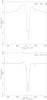 |
Fig. 5 Spectra of the 12CO(1-0) and 12CO(2-1) lines (with the continuum subtracted) toward the AGN of 3C 293. For clarity, we have zoomed into the velocity ranges where the emission is detected. |
4.2. Mass of molecular gas
The total 12CO(1-0) flux emitted by 3C 293 is 53 Jy km s-1. The equivalent 12CO(1-0) luminosity is L′CO = 4.8 × 10⁹ K km s-1 pc-2 (Solomon et al. 1997). Applying the Galactic ratio of H2-mass to CO-luminosity (4.6 M⊙/K km s-1 pc2Solomon et al. 1987), the H2 mass in 3C 293 is M(H2) = 2.2 × 10¹⁰M⊙. The column density of hydrogen atoms derived from CO is NH,CO = 2.8 × 1022 cm-2. Evans et al. (1999) measured a total 12CO(1-0) flux emitted by 3C 293 of 52 ± 11 Jy km s-1 in a 74″ diameter aperture, suggesting that we are including all CO emission of 3C 293 in our observations.
The dynamical mass (Mdyn) inside a radius, R, can be derived as  /G, where G is the gravitational constant, and νrot is the de-projected radial velocity at the edge of the disk. The fits to the velocity maps of 3C 293 (Sect. 4.4) show that the circular velocity of the CO disk is 251 km s-1 at R = 9.2″ (8 kpc). The inclination angle of the disk at that radius is i = 58° (Sect. 4.4). Therefore, νrot ≃ 300 km s-1, and Mdyn ≃ 2.0 × 10¹¹M⊙. Removing the mass of molecular gas derived above and neglecting the contribution from dark matter, the spheroidal stellar mass within R = 8 kpc is Msph ≃ 1.8 × 10¹¹M⊙, consistent with the total stellar mass derived from stellar population fits to the optical spectra (2.8 × 10¹¹M⊙, Tadhunter et al. 2011), and the Mbulge derived from optical photometry (Bettoni et al. 2003).
 |
Fig. 6 12CO(1-0) (left) and 12CO(2-1) (right) velocity maps of 3C 293. Velocities are given in km s-1 with respect to |
4.3. Determination of the systemic velocity
The first measurements of the vsys of 3C 293 were made by Sandage (1966) and Burbidge (1967). Using optical emission lines, they obtained vsys = 13 500 km s-1, which is also the central velocity of the deepest H i absorption. That value was adopted until 2005, when Emonts et al. (2005) used high-resolution long-slit spectra of the ionized gas emission lines to calculate the redshift of the narrow component of the optical emission lines in the nucleus of 3C 293: z = 0.048 6 ± 0.001 2,  450 ± 35 km s-1.
Our data resolve the whole molecular gas (and dust) disk that rotates around the AGN, which allows a new determination of the systemic velocity of 3C 293. Figure 5 shows that the 12CO(1-0) and 12CO(2-1) spectra of 3C 293 at the AGN consist of a combination of absorption and emission lines. Absorption lines can be formed in clouds with noncircular trajectories that cross in front of the AGN or jet. Estimations based on absorption lines, which are sensitive to a low column density of gas, may then yield incorrect values of the vsys. The CO emission lines of 3C 293, in contrast, are produced ubiquitously in the rotating disk. The inferred kinematic parameters, including vsys, are thus more representative of the majority of the molecular gas. Therefore, we used the 12CO(1-0) emission line (which has higher signal-to-noise ratio than the 12CO(2-1) line) toward the AGN to measure the vsys of 3C 293. After removing the absorption line from the spectrum, we averaged the velocities where the 12CO(1-0) emission line shows emission over 3σ, weighting them by the flux in each velocity channel, and obtained vsys = 13 437 ± 10 km s-1. A Gaussian fit of the emission line produces vsys = 13 435 ± 10 km s-1. Both values are consistent with  = 13 434 ± 8 km s-1derived from the kinematic analysis of the CO disk (see Sect. 4.4), and the optically derived
  . Hereafter, all velocities are given with respect to = 13 434 ± 8 km s-1.
4.4. Kinematics of the molecular gas
Figure 6 shows the 12CO(1-0) and 12CO(2-1) velocity maps of 3C 293. Based on these maps, the velocity fields of the 12CO(1-0) and 12CO(2-1) emission lines are consistent with a rotating disk where the northeastern side is receding and the southwest is approaching. The velocity field of the 12CO(1-0) line shows that the major axis of the disk is oriented along PAvel ~ 45° in the inner 7–8″ (radius), and shifts toward PAvel ~ 55° for larger distances, consistent with the PAmorph estimated from the 12CO(1-0) emission map (Sect. 4.1). Visual inspection of the 12CO(2-1) velocity field cannot confirm the ridge seen in the 12CO(2-1) line emission map at radius ~3–4″. The ridge is verified by the analytic study of the CO kinematics below.
 |
Fig. 7 Position–velocity diagram of the 12CO(1-0) (left panels) and 12CO(2-1) (right panels) emission along the major axis of the molecular gas disk (top panels) and AGN-jet line (bottom panels) of 3C 293. Positions (Δz′) are relative to the AGN. Velocities are relative to the |
Figure 7 shows the position−velocity (P − V) diagrams for the 12CO(1-0) and 12CO(2-1) lines taken along the major axis of the disk (PA = 45°), and along the AGN-jet line (PA = 89°). The P − V diagrams along the major axis are consistent with a CO-emitting, spatially resolved rotating molecular gas disk, with projected peak velocities of ±350 km s-1 at its edges. Both the 12CO(1-0) and 12CO(2-1)P − V diagrams show a spatially unresolved absorption feature centered on the AGN coordinates, with a width of ~100 km s-1, as seen in the CO spectra (Fig. 5). The P − V diagram of 12CO(1-0) along the AGN-jet line shows that the AGN absorption is spread by the beam up to the jet coordinates. The 12CO(2-1)P − V diagram shows two absorption features. The first one is detected between distances 0.4′′ and 1.6″ from the AGN, centered on –100 km s-1, with a width of ~100 km s-1. This feature corresponds to the blueshifted absorption detected toward the jet coordinates in the 12CO(2-1) spectrum. The second absorber is detected at the AGN coordinates, centered on velocities ~200 km s-1, corresponding to the narrow absorption feature seen in the 12CO(2-1) spectrum of the AGN (Fig. 5).
To analyze the kinematics of CO in 3C 293 in more detail, we used the IDL tool kinemetry (Krajnović et al. 2006). Kinemetry divides the 2D line-of-sight velocity map of a galaxy into a series of ellipses. Each of these ellipses has a velocity profile that is decomposed into a finite series of harmonic Fourier terms: ![Mathematical equation: \begin{equation} V = c_0(r) + \sum_{n=1}^{N} [c_n(r) \cos(n \psi) + s_n(r) \sin(n \psi)], \end{equation}](/articles/aa/full_html/2014/04/aa23123-13/aa23123-13-eq104.png) (1)where r is the radius of the ellipse, ψ the eccentric anomaly, and c0 the vsys. Krajnović et al. (2006) showed that to describe the velocity map, only terms up to N = 3 are needed. The circular (Vcirc) and noncircular (Vnc) velocities can be obtained using (Schoenmakers et al. 1997)
(1)where r is the radius of the ellipse, ψ the eccentric anomaly, and c0 the vsys. Krajnović et al. (2006) showed that to describe the velocity map, only terms up to N = 3 are needed. The circular (Vcirc) and noncircular (Vnc) velocities can be obtained using (Schoenmakers et al. 1997) ![Mathematical equation: \begin{equation} V_{\rm{circ}}=c_1 , \quad V_{\rm{nc}}=\sqrt[]{s_1^2+s_2^2+c_2^2+s_3^2+c_3^2} . \end{equation}](/articles/aa/full_html/2014/04/aa23123-13/aa23123-13-eq111.png) (2)To find the ellipse along which the velocity field should be extracted (the best-sampled ellipse), kinemetry minimizes Vnc2 (
(2)To find the ellipse along which the velocity field should be extracted (the best-sampled ellipse), kinemetry minimizes Vnc2 ( ; see also Carter 1978; Kent 1983; Jedrzejewski 1987). The best-sampled ellipse for a given radius is then given in terms of central coordinates, ellipticity, and PA.
 |
Fig. 8 Results of the fits with kinemetry for the inclination and position angles (top panels), the circular velocity (bottom-left panel), and the noncircular velocity (bottom-right panel). |
We set the ellipse radii in steps of 0.2″ for the 12CO(2-1) velocity field. For the 12CO(1-0) field we used ellipses every 0.5″ in the inner regions (<4″) and 1″ for the outer regions (>4″). The minimum radius was set to half the FWHM of the beam for both maps, and the centers of the ellipses were fixed at the AGN coordinates,which is implicitly assumed to be the dynamical center. For ellipses where the kinemetry fit did not converge, we allowed variations in the radius of ≲0.3″ until the fit converged. All the Fourier coefficients, including Vcirc, where left free to vary.
Figure 8 shows the kinemetry fits for the inclination and position angles, and the circular and noncircular velocities for 3C 293. The inclination angle plot shows two orientations: a roughly constant i ≃ 75° for radii below 3.8″, and an inclination angle increasing from 20° to 65° from a radius 4″ to 11″, suggesting a twist in the CO disk. Thus, our analysis confirms the orientation proposed by Floyd et al. (2006): the southeastern side of the disk is facing us, and the eastern jet of the compact radio source is approaching. The steep change in the inclination angle along radii 4′′ and 8′′ suggests that the CO disk is warped.
The position angle is roughly constant (PA ≃ 45°) for the 12CO(1-0) velocity field up to a radius of 8″. Beyond this radius, the diagram clearly shows a change in PA (≃55°), consistent with a warped CO disk. The PA fit of the 12CO(2-1) velocity map shows strong variations at small radii. These variations are likely due to small-scale structure of the velocity field and the presence of the central absorber, and not a global property of the disk. Between radii of 1″ and 2.5″, the PA of the 12CO(2-1) velocity field is consistent with the PA seen for 12CO(1-0). Beyond 2.5″, the PA is ~25°, consistent with the ridge seen in the 12CO(2-1) line emission map (Sect. 4.1 and Fig. 2). Hence, the fits of the inclination and position angles of 3C 293 support the scenario of a warped, corrugated CO disk.
The Vcirc increase with distance to the AGN, up to 240 km s-1 at a radius of ~4″. Beyond this radius we see a small dip in the curve followed by an increase with the distance up to 250 km s-1 at ~6–7″. Then, the circular velocity decreases with distance beyond 9″. The noncircular velocities (Vnc) constantly increase with distance all along the CO velocity field. Vnc shows a break point at radius 4′′.All changes in circular and noncircular velocities occur at radii where the inclination and position angles suggest a distortion in the disk, consistent with different stages of gas settling at each orientation of the disk.
The kinemetry fits give a total velocity (![Mathematical equation: \hbox{$\sqrt[]{V_{\rm{circ}}^2+V_{\rm{nc}}^2}$}](/articles/aa/full_html/2014/04/aa23123-13/aa23123-13-eq115.png) ) of 307 ± 33 km s-1 at R = 9″ (8.4 kpc). This corresponds to a de-projected velocity V = 361 ± 40 km s-1, compatible with the velocities observed in early-type galaxies (full width at zero intensity, FWZI ≲ 800 km s-1; e.g., Krips et al. 2010; Crocker et al. 2012, and references therein). As discussed above, kinemetry also fits the vsys for each ellipse of the velocity map. Based on the PA results of the 12CO(1-0) velocity map, we averaged the vsys fitted for each ellipse up to 8″. We obtained = 13 434 ± 8 km s-1, which is consistent with the vsys derived in Sect. 4.3.
) of 307 ± 33 km s-1 at R = 9″ (8.4 kpc). This corresponds to a de-projected velocity V = 361 ± 40 km s-1, compatible with the velocities observed in early-type galaxies (full width at zero intensity, FWZI ≲ 800 km s-1; e.g., Krips et al. 2010; Crocker et al. 2012, and references therein). As discussed above, kinemetry also fits the vsys for each ellipse of the velocity map. Based on the PA results of the 12CO(1-0) velocity map, we averaged the vsys fitted for each ellipse up to 8″. We obtained = 13 434 ± 8 km s-1, which is consistent with the vsys derived in Sect. 4.3.
The comparison of the first- and third-order sine coefficients of the Fourier decomposition (s1, s3) gives insights into the noncircular motions of the disk (Schoenmakers et al. 1997). Wong et al. (2004) showed that for a pure warp model, the s1, s3 data points follow  (3)with q = cos(i). Using the method by Wong et al. (2004), we aimed to confirm the warped morphology in 3C 293 by searching the kinematics of the gas for deviations from the disk rotation. We ran kinemetry a second time, fixing the inclination and position angle to their average values at the inner radii (R< 6″) obtained in the first kinemetry run (77° and 45°, respectively). Figure 9 shows the s1/c1 and s3/c1 values obtained from this second kinemetry run. If there is a warp, s1/c1 and s3/c1 should follow a correlation with slope δs3/δs1 = 0.83. This slope is illustrated in Fig. 9 with a black dashed line. The 12CO(2-1) data clearly have the warp-line slope for radii R ≥ 2.8″. For the 12CO(1-0) line, this behavior is seen between radii 4″ and 10″ and beyond R ≥ 10.8″, consistent with the scenario of a large-scale warp in the CO disk of 3C 293.
5. Is there a molecular gas outflow in 3C 293?
The radio and optical spectra of 3C 293 show broad (~1000 km s-1) components in the H i absorption and ionized gas emission lines generated by fast gas outflows near (≲1 kpc) the AGN. These outflows seem to be produced by the interaction between the radio jets of the inner radio source and the ISM of the host galaxy (Morganti et al. 2003b; Emonts et al. 2005; Mahony et al. 2013).
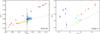 |
Fig. 9 Comparison of the s3/c1 and s1/c1 ratios of the Fourier coefficients from the kinemetry fits. Radii increase from blue to red. The distance between two adjacent radii is 0.2″. The dashed line shows the slope of the correlation expected for a warp (Wong et al. 2004). |
Figure 10 shows the overlay of the 12CO(1-0) and 12CO(2-1) spectra toward the AGN eastern jet and CO disk regions, with the spatially unresolved H i spectrum (Morganti et al. 2003b). All the CO spectra show emission consistent with a FWHM of ~300–350 km s-1 Gaussian, combined with a strong, structured absorption feature. The central 12CO(1-0) and 12CO(2-1) absorptions at the AGN and the 12CO(1-0) absorption at the jet show a similar structure, with central velocities v – ~ +40 km s-1, and a FWHM of ~60 km s-1. This absorption feature consists of two components separated by ~40 km s-1, with FWHM ~ 20–30 km s-1. The AGN spectra for the 12CO(1-0) and 12CO(2-1) lines also show a narrow (FWHM ≃ 30 km s-1) absorption line at v – ~ +200 km s-1. The 12CO(2-1) absorption at the coordinates of the jet has a FWHM of ≃80 km s-1, and it is ~10 times fainter and blueshifted by ~100 km s-1 with respect to the central absorptions in the rest of the spectra.
The H i spectrum of 3C 293 shows absorption features against the jets of the compact radio source, which seem to be produced by absorbers in the dust disk (Baan & Haschick 1981; Haschick & Baan 1985; Beswick et al. 2002, 2004; Floyd et al. 2006). Figure 11 shows the overlay of the 12CO(1-0) and H iP − V diagrams along the AGN-jet line (PA = 89°), and the location of the H i outflow. The H i absorption toward the core is centered on v – ~ +50 km s-1 and has FWHM ~ 80 km s-1, consistent with the CO absorption at the same coordinates. The 12CO(1-0) beam covers all of the eastern jet radio lobe (regions 1 through 6 in Beswick et al. 2004, see also the IR jet lobes in Fig. 4). At these coordinates, the H i spectrum shows absorptions with centers ranging from v – = − 100 km s-1 to 60 km s-1, and FWHM from 20 to 50 km s-1. All the CO absorption features seen toward the jet and core of 3C 293 are associated with the H i absorption components that originated in the disk. The CO spectra show no indications of outflowing molecular gas either in the absorption or emission lines.
As discussed in the previous section, the kinematics of CO in 3C 293 is consistent with a large, corrugated, warped disk with circular rotation around the core. The bottom panels of Fig. 10 show that ~400 km s-1 of the H i outflow component cannot be explained by rotation of the disk. None of the CO lines show traces of outflowing molecular gas in 3C 293 either in absorption or emission at the velocities of the H i outflow anywhere in the galaxy (see also Fig. 11). It should be noted that our data do not have the spatial resolution needed to separate the spectra of the AGN and the western jet lobe, where the H i outflow has been detected. Therefore we used our AGN spectrum to establish a limit on the mass of the CO outflow in 3C 293. Based on the 12CO(1-0) spectrum, the 3σ upper limit to the molecular gas mass of a 400 km s-1 cold-H2 emission outflow is ≲7.1 × 10⁸M⊙, that is, 3.2% of the total of cold-H2 mass. For comparison, the mass ratio of the outflow detected in Mrk 231 is 6% (Feruglio et al. 2010; Cicone et al. 2012), almost twice as high as the 3σ upper limit for 3C 293; the ratio measured in NGC 1266 is 2.2% (Alatalo et al. 2011), and the ratio for IC 5063 is somewhere between 4.5–26% (Morganti et al. 2013). Mahony et al. (2013) estimated that the mass outflow rate of the H i outflow is Ṁ = 8 − 50M⊙ yr -1, assuming velocities between 100 and 600 km s-1 for the gas. If we compare the CO and H i spectra in the region where the H i outflow was detected (Fig. 11), the H i outflow velocities beyond the rotation of the disk range from ~–300 to ~–900 km s-1, with respect to (i.e. voutflow = 0–600 km s-1), which yields an average outflow rate Ṁ ≃ 25–30 M⊙ yr -1.
6. Star formation properties of 3C 293
Nesvadba et al. (2010) found that powerful radio galaxies show an SFR surface density lower by 10 to 50 times than normal star-forming galaxies with the same molecular gas surface density. They calculated the SFR using the 7.7 μm PAH feature emission of their sample, except for 3C 326 N, where they also used the 70 μm continuum emission as an SFR estimator (Ogle et al. 2007). Nesvadba et al. (2010) suggested that the low SFR in radio galaxies is due to a lower star-forming efficiency (SFE = SFR/M(H2)) than in normal galaxies. Large-scale shocks in the ISM of radio galaxies may increase the turbulence of molecular gas (see also Nesvadba et al. 2011), which inhibits star formation to a large extent.
In Sect. 6.1, we calculate the SFR of 3C 293 using all available estimators. Some SFR tracers are sensitive to AGN radiation and jet-induced shocks in the ISM, because these may increase the flux of ionized gas emission lines, vary the shape of the continuum, and destroy ISM molecules such as the PAH. Hence, we also discuss the possible caveats of the different SFR calibrations to find the most accurate value of the SFR for 3C 293. In Sect. 6.2, we study the SFE and the location of 3C 293 in the Kennicut-Schmidt (KS) diagram and discuss the differences with respect to the results obtained by Nesvadba et al. (2010). We complete the comparison sample with the young radio sources 4C 12.50, 4C 31.04 (Willett et al. 2010), and the reactivated radio source 3C 236 (Tremblay et al. 2010; Labiano et al. 2013).
6.1. Star formation rate
 |
Fig. 10 Overlays of the spatially unresolved H i (Morganti et al. 2003b) spectrum and the 12CO(1-0) and 12CO(2-1) spectra (with the continuum subtracted) toward the AGN, eastern jet, and disk regions of 3C 293. The CO spectra correspond to the regions of the AGN (top panels), jet (2nd row), and 12CO(1-0) and 12CO(2-1) emission disks (3rd row). The green-shaded area marks the area of the H i absorption that cannot be attributed to rotation around the AGN. Fluxes are in arbitrary units. Velocities are given with respect to |
6.1.1. Near-ultraviolet photometry
Figure 12 shows an overlay of the HST-NUV image and the CO maps of 3C 293. The morphology of the UV emission, which shows a highly clumpy distribution, indicates that most of the UV knots are associated with star formation (Allen et al. 2008; Baldi & Capetti 2008). Inspection of Fig. 12 suggests that the star-forming regions are associated with the CO disk. The heavy obscuration seen in the R − H map, and the patchy morphology of the NUV emission suggest that any SFR estimations based on the NUV image will be largely underestimated, however, and we therefore preferred not to use it to calculate the SFR.
6.1.2. Optical spectroscopy
The optical spectra available for 3C 293 are from the central 3″ of the source. In this region we can expect a large contribution from the AGN to the emission lines used to trace the SFR (e.g., Hα and O ii, Kennicutt 1998b), which would cause an overestimated SFR value. On the other hand, the nuclear region of 3C 293 is crossed by large, thick, dust lanes, which absorb a large amount of optical emission-line flux. Thus, any SFR evaluation based on optical fluxes will be underestimated. The combination of both effects (overestimation due to the AGN emission, and underestimation due to dust obscuration) makes it impossible to calculate the contribution from star-forming regions to the optical emission line fluxes in the nucleus of 3C 293.
6.1.3. Mid-infrared continuum
Calzetti et al. (2007) showed that the 24 μm luminosity of a galaxy is indicative of its SFR (see also Rieke et al. 2009; Kennicutt et al. 2009; Calzetti et al. 2010). They presented two SFR calibrations: based on the 24 μm luminosity alone, and combined with the Hα luminosity. If we apply these calibrations to the 24 μm emission of 3C 293 (F24 μm = 3.88 × 10⁻¹² erg s-1 cm-2, Dicken et al. 2010), and the Hα emission of 3C 293 (FHα = 9.83 × 10⁻¹⁵erg s-1 cm-2; SDSS, Buttiglione et al. 2010), we obtain an SFR = 3.0M⊙ yr-1 and an SFR = 3.2 ± 0.1 M⊙ yr-1for the 24 μm and 24 μm+Hα, respectively. A possible caveat of the 24 μm emission as SFR estimator is that this emission can be increased by the heating of dust by the AGN (Tadhunter et al. 2007), yielding an overestimated SFR. However, Leipski et al. (2009) found that the Spitzer IRS spectrum of 3C 293 is dominated by star formation, and the shape of the continuum is similar to the continuum of local star-forming galaxies (e.g., Smith et al. 2007). Therefore the SFR obtained from the 24 μm emission is a good estimator of the global SFR of the obscured star-forming regions in 3C 293.
 |
Fig. 11 Overlay of the 12CO(1-0) (contours) and the H i (Fig. 1 from Mahony et al. 2013, gray scale) P − V diagrams along the AGN-jet line (PA = 89°). Positions (Δz′) are relative to the AGN. Velocities are relative to the |
The 70 μm luminosity can be used to establish lower and upper limits on the SFR (Seymour et al. 2011; Symeonidis et al. 2008; Kennicutt 1998a). The lower limit is obtained by subtracting the AGN contribution from the 70 μm luminosity with the [O iii] and 70 μm correlation by Dicken et al. (2010). The upper limit is obtained assuming that all the 70 μm emission is due to star formation. Using the 70 μm flux of 3C 293 measured by Dicken et al. (2010) with Spitzer (F70 μm = 1.29 × 10⁻¹¹ erg s-1 cm-2), we obtained 5.8 <SFR< 6.0 M⊙ yr -1. The 70 μm emission can be increased by the heating of dust by the AGN (Tadhunter et al. 2007), which would give an overestimated SFR. For 3C 293, Dicken et al. (2010) found that the 70 μm emission is ~35 times brighter than expected for a nonstarburst galaxy with the same [O iii] luminosity. The authors showed that this difference arises because star formation is the main contributor to the 70 μm flux. The SFR derived from 70 μm for 3C 293 is consistent with the SFR derived from the 24 μm emission, which supports the assumption that the contribution from the AGN to these fluxes is low, and the SFR estimations from the IR continuum are accurate.
6.1.4. Mid-infrared spectroscopy
Based on a sample of 25 Seyfert galaxies, Diamond-Stanic & Rieke (2010) found that the [Ne ii] emission line is a good tracer of the SFR in AGN. Willett et al. (2010) used the [Ne iii]λ15.6 μm plus the [Ne ii]λ12.8 μm fluxes to measure the SFR in a sample of compact symmetric objects (CSO, see also Ho & Keto 2007). The neon emission lines of 3C 293 have fluxes F[Ne ii] = (4.07 ± 1.29) × 1010 erg s-1 cm-2 and F[Ne iii] = (1.27 ± 0.09) × 1010 erg s-1 cm-2 (Spitzer spectrum, Guillard et al. 2012), which yield SFR = 4.4 ± 1 M⊙ yr-1 and SFR = 11 ± 1M⊙ yr-1for the [Ne ii] and [Ne ii]+[Ne iii] relations, respectively.
The AGN contribution to the [Ne ii] line luminosity can be estimated with the [O iv]λ25.9 μm/[Ne ii] λ12.8 μm or the [Ne v]λ14.3 μm/[Ne ii]λ12.8 μm ratios (Diamond-Stanic & Rieke 2010; Sturm et al. 2002; Genzel et al. 1998). For 3C 293, the [O iv]/[Ne ii] and [Ne v]/[Ne ii] ratios are 0.07 and 0.04, respectively. Both values yield an AGN contribution below 10% to the [Ne ii] line (90% starburst contribution), consistent with the results obtained by Leipski et al. (2009) using the whole Spitzer IRS spectrum of 3C 293. The higher SFR from the combined neon lines is probably due to contributions from the AGN to the [Ne iii] line emission (LaMassa et al. 2012). Another estimate of the AGN contribution is given by the ratio [Ne iii]/[Ne ii], which increases with the hardness of the ionizing environment. For 3C 293, log [Ne iii]/[Ne ii] = –0.5, similar to the mean value of the ratio in ULIRG and starburst galaxies (–0.35), and below the mean value for AGN (–0.07) and CSO (–0.16, Willett et al. 2010), suggesting a low contribution from the AGN in 3C 293. Pereira-Santaella et al. (2010) studied the IR emission line ratios in a large sample of active and H ii galaxies. Based on their results, the [O iv]/[Ne ii] and [Ne iii]/[Ne ii] ratios of 3C 293 are closer to those of LINER-like and HII galaxies than Seyferts or quasi-stellar objects. Therefore, the flux of the [Ne ii] line of 3C 293 has negligible contributions from the AGN, and it is a reliable SFR estimator.
 |
Fig. 12 HST-NUV image of 3C 293, with the 12CO(1-0) (left) and 12CO(2-1) (right) emission overlaid. Contour levels as in Fig. 3. Color version available in electronic form. HST image in counts s-1. |
 |
Fig. 13 Spitzer/IRAC 8 μm map of 3C 293, with the 12CO(1-0) and 12CO(2-1) emission overlaid. Contour levels as in Fig. 3. Color version available in electronic form. |
6.1.5. PAH emission
The mid-IR spectrum of 3C 293 shows clear emission lines from several PAH features: F11 μm = (2.15 ± 0.06) × 10-13 erg s-1 cm-2, F7.7 μm = (5.57 ± 0.25) × 10-13 erg s-1 cm-2 and F6.2 μm = (1.11 ± 0.06) × 10-13 erg s-1 cm-2 (Dicken et al. 2012; Guillard et al. 2012).
Based on the correlation found between the emission of the neon line and the 6.2 μm plus 11.3 μm PAH, Willett et al. (2010) used the luminosities of these PAH to calculate the SFR in their sample (see also Farrah et al. 2007). Applying this method to 3C 293 (F6.3 + 11.3 μm = (3.26 ± 0.12) × 10-13 erg s-1 cm-2), we obtained SFR = 18 ± 1 M⊙ yr -1.
By combining Eqs. (2), (3) and (8) of Calzetti et al. (2007), a relation between S8 μm,dust and SFR can be derived (see e.g., Nesvadba et al. 2010); where S8 μm,dust is the luminosity surface density in the IRAC 8 μm image with the stellar continuum removed using the IRAC 3.6 μm image (Helou et al. 2004; Calzetti et al. 2005). Both the 8 μm and 3.6 μm IRAC images of 3C 293 are available in the Spitzer archive. We downloaded them and obtained an S8 μm,dust image4. To estimate the SFR, we divided 3C 293 into six different regions based on its NUV and CO morphology (the details can be found in Appendix A) and derived the SFR in each region. The results are summarized in Table 2. Our SFR estimates from S8 μm,dust are on average ~six times higher than the value obtained by Nesvadba et al. (2010). Nesvadba et al. (2010) calculated the SFR using the flux of the 7.7 μm PAH line from the Spitzer nuclear spectrum of 3C 293 (Ogle et al. 2010) as S8 μm,dust in the Calzetti et al. (2007) equations. The flux of the 7.7 μm PAH line was measured using PAHFIT (Smith et al. 2007). It should be noted that this flux estimate may be off by a factor ≲2 due to the extended PAH emission of 3C 293 (Ogle et al. 2010), while the IRAC image includes the whole extension of the PAH emission. In our analysis, we used the complete bandpass of the 8 μm IRAC image (6.4 to 9.3 μm, Fig. 13), corrected for the stellar continuum, as done by Calzetti et al. (2007).Inspection of the mid-infrared spectrum of 3C 293 shows that the 7.7 μm PAH line emission represents only ≲15% of the nuclear flux in the 8 μm IRAC band (e.g., Ogle et al. 2010; Guillard et al. 2012). Therefore, the origin the discrepancy with the Nesvadba et al. (2010) results seems to be the different fluxes considered for S8 μm,dust. Using the 7.7 μm PAH flux as S8 μm,dust underestimates the SFR of 3C 293.
Diamond-Stanic & Rieke (2010) found that the 11.3 μm PAH emission, by itself, is a reliable estimator of the SFR in Seyfert galaxies, unlike the 6.3 and 7.7 μm PAH (see also Smith et al. 2007; Diamond-Stanic & Rieke 2012; Esquej et al. 2014). They found a strong correlation between the emission of the [Ne ii] and 11.3 μm lines in their sample due to the star formation of the host galaxies, with no contributions from the AGN. By comparing the [Ne ii] and 11.3 μm PAH emission of 3C 293 with their sample (Fig. 5 of their paper), it is clear that the emission of 3C 293 is consistent with that correlation5. Using the 11.3 μm emission of 3C 293, we obtain a reliable estimation for the SFR of 3C 293: SFR = 2.5 ± 0.2 M⊙ yr -1.
6.2. Star formation efficiency
As discussed above, the most accurate SFR tracers for 3C 293 are the 11.3 μm PAH, and [Ne ii] emission lines and the 24 μm, 70 μm continuum emission, which yield an average SFR of 4.0 ± 1.5 M⊙ yr -1. Therefore, SFE3C 293 = 0.18 Gyr-1, and tdeplete ~ 5.6 Gyr. The average mass rate of the H i outflow is Ṁ ≃ 25–30 M⊙ yr -1 (Sect. 5), suggesting that the outflow might deplete the gas reservoir faster than the star formation, lowering the SFE of 3C 293. Figure 14 compares the canonical KS-law fitted for normal star-forming galaxies (Roussel et al. 2007; Kennicutt 1998b) with the SFR surface density (ΣSFR = SFR/area) and cold-H2 mass surface density (ΣMH2 = M(H2)/area) for 3C 293, the young sources 4C 12.50, 4C 31.04 (Willett et al. 2010), the re-started source 3C 236 (Labiano et al. 2013), and the sample of Nesvadba et al. (2010)6. Inspection of Fig. 14 shows that 3C 293 is a normal-efficiency (consistent with the KS-law) star-forming radio galaxy and is 10–50 times more efficient than the sample of Nesvadba et al. (2010). This means that the outflow seen in H i and ionized gas does not seem to affect the molecular-gas-forming stars.
The ΣSFR given by Nesvadba et al. (2010) for 3C 293 (labeled 3C 293-N10 in Fig. 14) is lower by a factor 2.5 than our ΣSFR estimates using S8 μm,dust, the 11 μm PAH and the [Ne ii] emission line. Inspection of Fig. 14 shows that increasing the ΣSFR of 3C 293-N10 by a 2.5 factor does not make it consistent with the KS-law, however. The ΣMH2 would be too large compared with our results. Nesvadba et al. (2010) used the M(H2) data published by Evans et al. (1999) to calculate the column density of H2 in 3C 293. Combining their single-dish and 3.5′′-resolution map of the 12CO(1-0) emission, Evans et al. (1999) argued that the 1010M⊙ of H2 are distributed along a ~7′′ (6 kpc) diameter disk, yielding a surface density ΣMH2 = 7.1 × 10⁸M⊙ yr -1/kpc-2. Our higher resolution and sensitivity 12CO(1-0) map shows that the molecular gas is distributed along a ~24″ (21 kpc-) diameter disk, with an average density of ΣMH2 = 6.4 × 10⁸M⊙ yr -1 kpc-2. Applying the latter density to 3C 293-N10 gives an SFE consistent with the KS-law.
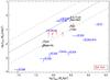 |
Fig. 14 ΣSFR and ΣMH2 of 3C 293 (black and red), the sample of Nesvadba et al. (2010) (blue diamonds), young sources 4C 12.50, 4C 31.04, and 3C 236 (blue stars). Red diamonds show the Spitzer S8 μm,dust data for 3C 293. Black diamonds show the SFR estimates for 3C 293 using the rest of tracers discussed in the text. DRNe2 and DR11 show the SFR estimates using the recipes of Diamond-Stanic & Rieke (2012), DS70 is the SFR estimate based on the method of Seymour et al. (2011), Dicken et al. (2010). Solid line: best-fit of the KS-law from Kennicutt (1998b). Dashed lines: dispersion around the KS-law best fit for normal star-forming galaxies (Roussel et al. 2007; Kennicutt 1998b). |
Our previous study of feedback in radio galaxies (Labiano et al. 2013) showed that the young (≲105 yr) radio sources 3C 236, 4C 12.50, and 4C 31.04 had an unexpectedly high SFE compared with the evolved (≳107 yr) radio galaxies in the sample of Nesvadba et al. (2010). Based on the age of these sources, we proposed an evolutionary scenario where the impact of AGN feedback on the ISM of the host galaxy would increase with the age of the radio source. Hence, older radio sources would show lower SFE than young sources. The large radio jets of 3C 293 have been active for the past ~2 × 10⁷ yr, which gives enough time for the feedback effects (such as an outflow) to spread across the ISM and suppress the star formation in the host. The SFE of 3C 293 is consistent with that of normal star-forming galaxies and young radio sources, with no evidence of quenched star formation, however. Therefore, the evolutionary scenario proposed in Labiano et al. (2013) does not seem to apply for 3C 293. Moreover, a recent study of the SED (from UV to radio wavelengths) of radio-loud AGN found that the SFR in these systems is mildly diminished by the radio jets, but similar (or higher) to the SFR of inactive galaxies (Karouzos et al. 2013). Our results suggest that the apparently low SFE found in evolved radio galaxies is probably caused by an underestimation of the SFR and/or an overestimation of the H2 density and is not a property of these sources.
7. Summary and conclusions
We carried out 1 mm, 3 mm continuum and 12CO(1-0), 12CO(2-1) line PdBI observations of the powerful radio galaxy 3C 293. The host of 3C 293 was known to harbor active star-forming regions and outflows on H i and ionized gas. The high sensitivity and resolution of our data in combination with HST and Spitzer images and H i spectra allowed us to study the impact of AGN feedback on the host of this evolved radio galaxy in detail. We investigated the kinematics and distribution of the molecular gas to search for evidence of outflow motions. We also accurately determined the SFE of the host galaxy and compared it with the efficiencies of normal star-forming galaxies and young and old radio sources. The main results of our work are summarized below:
-
The 1 mm and 3 mm maps separate the continuum emission from the AGN and the eastern jet of 3C 293. The emission of the AGN and jet at 1 mm and 3 mm are consistent with synchrotron radiation.
-
The cold molecular gas of 3C 293, traced by the 12CO(1-0) emission, forms a disk with a diameter of 21 kpc, with a mass M(H2) = 2.2 × 10¹⁰M⊙. The dust mapped by the HST R–H image and the star formation seen in the HST-NUV and Spitzer-8 μm images are clearly associated with the molecular gas disk. The morphology of the CO emission is consistent with a warped, corrugated disk, with the outer edges (R ≳ 8 kpc) seen almost edge-on, and the central (R ≲ 4 kpc) region tilted toward the plane of the sky, with the southern side facing us.
-
The kinematics of the CO disk is consistent with rotation around the core, with no evidence of fast (≳500 km s-1) outflowing molecular gas. The detailed analysis of the CO kinematics showed that the inclination and the position angle of the disk are consistent with a corrugated, warped morphology. Furthermore, the Fourier decomposition of the velocity field is consistent with the presence of a warp in the CO disk of 3C 293, as suggested by the CO maps. Using the kinematics of the 12CO(1-0) emission line, we determined the systemic velocity of 3C 293 to be
= 13 434 ± 8 km s-1. -
The CO spectra of 3C 293 reveal several CO absorption features toward the core and jet coordinates. These absorptions are consistent with those observed in the H i spectra, which originate in the disk. The comparison of the CO and H i spectra also showed that the velocities of the H i outflow that cannot be explained by rotation of the disk range from ~300 km s-1 to ~900 km s-1 with respect to the systemic velocity.
-
We studied the different SFR tracers available for 3C 293, from NUV to IR, to obtain an accurate estimate of its SFR. The most reliable tracers are the [Ne ii] and 11.3 μm PAH emission, as well as the 24 and 70 μm continuum, which, for 3C 293, have negligible AGN contributions. The average SFR value for 3C 293 is 4.0 ± 1.5 M⊙ yr -1.
-
The SFE of 3C 293 (SFE = 0.18 Gyr-1) is consistent with the KS-law of normal galaxies and young radio galaxies. It is 10–50 times higher than the efficiencies measured in other evolved radio galaxies. Therefore, the evolutionary scenario of AGN feedback proposed in our previous work (Labiano et al. 2013) does not apply to the evolved radio galaxy 3C 293. The higher SFE of 3C 293 is a global property of the molecular gas disk.
-
The origin of the discrepancy between the SFE of powerful radio galaxies and normal, KS-law, star-forming galaxies, might be due to the use of the 7.7 μm PAH emission, which probably underestimates the SFR in powerful AGN environments, and/or an underestimation of the H2 surface densities in radio galaxies.
3C 293 also shows properties of an FR I radio galaxy. In the literature, it is sometimes classified as an FR I or intermediate FR I/II radio galaxy (e.g., Leipski et al. 2009; Massaro et al. 2010; Tadhunter et al. 2011).
The total mass of dust in UGC 8782 is ~ 107M⊙ (de Koff et al. 2000; Papadopoulos et al. 2010).
For our data, the variations in the f3.6 factor of the correction (0.22−0.29 Helou et al. 2004) do not affect the results noticeably.
LaMassa et al. (2012) found that the 11.3 μm PAH is significantly suppressed in AGN-dominated systems. However, this may not apply to 3C 293, because it is a starburst-dominated system (Dicken et al. 2010; Leipski et al. 2009).
The data from Nesvadba et al. (2010) did not include warm-H2. Therefore, we considered only the cold-H2 mass for the comparison of star-formation laws, which yields log ΣMH2 ≃ 7.7 M⊙ kpc-2. Adding the cold and warm-H2 masses of 3C 293 yields log ΣMH2 ≃ 7.9 M⊙ kpc-2.
Acknowledgments
We are grateful to A. Alonso-Herrero, P. Esquej, N. Nesvadba, E. Bellocchi and K. Dasyra for fruitful scientific discussions. We also thank the anonymous referee for very useful comments and suggestions. AL acknowledges support by the Spanish MICINN within the program CONSOLIDER INGENIO 2010, under grant ASTROMOL (CSD2009-00038), Springer and EAS. This research has made use of NASA’s Astrophysics Data System Bibliographic Services and of the NASA/IPAC Extragalactic Database (NED) which is operated by the Jet Propulsion Laboratory, California Institute of Technology, under contract with the National Aeronautics and Space Administration. Based on observations made with the NASA/ESA Hubble Space Telescope, and obtained from the Hubble Legacy Archive, which is a collaboration between the Space Telescope Science Institute (STScI/NASA), the Space Telescope European Coordinating Facility (ST-ECF/ESA) and the Canadian Astronomy Data Centre (CADC/NRC/CSA). Funding for the SDSS and SDSS-II has been provided by the Alfred P. Sloan Foundation, the Participating Institutions, the National Science Foundation, the United States Department of Energy, NASA, the Japanese Monbukagakusho, the Max-Planck Society, and the Higher Education Funding Council for England. The SDSS website is http://www.sdss.org/. The SDSS is managed by the Astrophysical Research Consortium for the Participating Institutions. The Participating Institutions are the American Museum of Natural History, Astrophysical Institute Potsdam, University of Basel, University of Cambridge, Case Western Reserve University, University of Chicago, Drexel University, Fermilab, the Institute for Advanced Study, the Japan Participation Group, Johns Hopkins University, the Joint Institute for Nuclear Astrophysics, the Kavli Institute for Particle Astrophysics and Cosmology, the Korean Scientist Group, the Chinese Academy of Sciences (LAMOST), Los Alamos National Laboratory, the Max-Planck Institute for Astronomy (MPIA), the Max-Planck Institute for Astrophysics (MPA), New Mexico State University, Ohio State University, University of Pittsburgh, University of Portsmouth, Princeton University, the United States Naval Observatory and the University of Washington. This work makes use of euro-vo software, tools or services and TOPCAT (Taylor 2005). Euro-vo has been funded by the European Commission through contract numbers RI031675 (DCA) and 011892 (VO-TECH) under the Sixth Framework Programme and contract number 212104 (AIDA) under the Seventh Framework Programme.
References
- Aalto, S., Garcia-Burillo, S., Muller, S., et al. 2012, A&A, 537, A44 [NASA ADS] [CrossRef] [EDP Sciences] [Google Scholar]
- Abazajian, K. N., Adelman-McCarthy, J. K., Agüeros, M. A., et al. 2009, ApJS, 182, 543 [NASA ADS] [CrossRef] [Google Scholar]
- Akujor, C. E., Leahy, J. P., Garrington, S. T., et al. 1996, MNRAS, 278, 1 [NASA ADS] [CrossRef] [Google Scholar]
- Alatalo, K., Blitz, L., Young, L. M., et al. 2011, ApJ, 735, 88 [NASA ADS] [CrossRef] [Google Scholar]
- Allen, M. G., Sparks, W. B., Koekemoer, A., et al. 2002, ApJS, 139, 411 [NASA ADS] [CrossRef] [Google Scholar]
- Allen, M. G., Groves, B. A., Dopita, M. A., Sutherland, R. S., & Kewley, L. J. 2008, ApJS, 178, 20 [Google Scholar]
- Baan, W. A., & Haschick, A. D. 1981, ApJ, 243, L143 [NASA ADS] [CrossRef] [Google Scholar]
- Baldi, R. D., & Capetti, A. 2008, A&A, 489, 989 [NASA ADS] [CrossRef] [EDP Sciences] [Google Scholar]
- Best, P. N., Kaiser, C. R., Heckman, T. M., & Kauffmann, G. 2006, MNRAS, 368, L67 [NASA ADS] [Google Scholar]
- Beswick, R. J., Pedlar, A., & Holloway, A. J. 2002, MNRAS, 329, 620 [NASA ADS] [CrossRef] [Google Scholar]
- Beswick, R. J., Peck, A. B., Taylor, G. B., & Giovannini, G. 2004, MNRAS, 352, 49 [NASA ADS] [CrossRef] [Google Scholar]
- Bettoni, D., Falomo, R., Fasano, G., & Govoni, F. 2003, A&A, 399, 869 [NASA ADS] [CrossRef] [EDP Sciences] [Google Scholar]
- Bîrzan, L., Rafferty, D. A., McNamara, B. R., Wise, M. W., & Nulsen, P. E. J. 2004, ApJ, 607, 800 [NASA ADS] [CrossRef] [Google Scholar]
- Burbidge, E. M. 1967, ApJ, 149, L51 [NASA ADS] [CrossRef] [Google Scholar]
- Burbidge, G., & Crowne, A. H. 1979, ApJS, 40, 583 [NASA ADS] [CrossRef] [EDP Sciences] [Google Scholar]
- Buttiglione, S., Capetti, A., Celotti, A., et al. 2009, A&A, 495, 1033 [NASA ADS] [CrossRef] [EDP Sciences] [Google Scholar]
- Buttiglione, S., Capetti, A., Celotti, A., et al. 2010, A&A, 509, A6 [NASA ADS] [CrossRef] [EDP Sciences] [Google Scholar]
- Calzetti, D., Kennicutt, Jr., R. C., Bianchi, L., et al. 2005, ApJ, 633, 871 [NASA ADS] [CrossRef] [Google Scholar]
- Calzetti, D., Kennicutt, R. C., Engelbracht, C. W., et al. 2007, ApJ, 666, 870 [NASA ADS] [CrossRef] [Google Scholar]
- Calzetti, D., Wu, S.-Y., Hong, S., et al. 2010, ApJ, 714, 1256 [NASA ADS] [CrossRef] [Google Scholar]
- Capetti, A., de Ruiter, H. R., Fanti, R., et al. 2000, A&A, 362, 871 [NASA ADS] [Google Scholar]
- Carter, D. 1978, MNRAS, 182, 797 [NASA ADS] [CrossRef] [Google Scholar]
- Cicone, C., Feruglio, C., Maiolino, R., et al. 2012, A&A, 543, A99 [NASA ADS] [CrossRef] [EDP Sciences] [Google Scholar]
- Cid Fernandes, R., Mateus, A., Sodré, L., Stasińska, G., & Gomes, J. M. 2005, MNRAS, 358, 363 [NASA ADS] [CrossRef] [Google Scholar]
- Ciotti, L., & Ostriker, J. P. 2007, ApJ, 665, 1038 [NASA ADS] [CrossRef] [Google Scholar]
- Colla, G., Fanti, C., Fanti, R., et al. 1975, A&AS, 20, 1 [NASA ADS] [Google Scholar]
- Crenshaw, D. M., Schmitt, H. R., Kraemer, S. B., Mushotzky, R. F., & Dunn, J. P. 2010, ApJ, 708, 419 [Google Scholar]
- Crocker, A., Krips, M., Bureau, M., et al. 2012, MNRAS, 421, 1298 [NASA ADS] [CrossRef] [Google Scholar]
- Croton, D. J., Springel, V., White, S. D. M., et al. 2006, MNRAS, 365, 11 [NASA ADS] [CrossRef] [Google Scholar]
- Dasyra, K. M., & Combes, F. 2011, A&A, 533, L10 [NASA ADS] [CrossRef] [EDP Sciences] [Google Scholar]
- Dasyra, K. M., & Combes, F. 2012, A&A, 541, L7 [NASA ADS] [CrossRef] [EDP Sciences] [Google Scholar]
- de Koff, S., Best, P., Baum, S. A., et al. 2000, ApJS, 129, 33 [NASA ADS] [CrossRef] [Google Scholar]
- de Vaucouleurs, G., de Vaucouleurs, A., Corwin, Jr., H. G., et al. 1991, Third Reference Catalogue of Bright Galaxies, Volume 1–3 (Berlin, Heidelberg, New York: Springer-Verlag) [Google Scholar]
- Di Matteo, T., Springel, V., & Hernquist, L. 2005, Nature, 433, 604 [NASA ADS] [CrossRef] [PubMed] [Google Scholar]
- Diamond-Stanic, A. M., & Rieke, G. H. 2010, ApJ, 724, 140 [NASA ADS] [CrossRef] [Google Scholar]
- Diamond-Stanic, A. M., & Rieke, G. H. 2012, ApJ, 746, 168 [Google Scholar]
- Dicken, D., Tadhunter, C., Axon, D., et al. 2010, ApJ, 722, 1333 [NASA ADS] [CrossRef] [Google Scholar]
- Dicken, D., Tadhunter, C., Axon, D., et al. 2012, ApJ, 745, 172 [NASA ADS] [CrossRef] [Google Scholar]
- Emonts, B. H. C., Morganti, R., Tadhunter, C. N., et al. 2005, MNRAS, 362, 931 [NASA ADS] [CrossRef] [Google Scholar]
- Esquej, P., Alonso-Herrero, A., González-Martín, O., et al. 2014, ApJ, 780, 86 [Google Scholar]
- Evans, A. S., Sanders, D. B., Surace, J. A., & Mazzarella, J. M. 1999, ApJ, 511, 730 [NASA ADS] [CrossRef] [Google Scholar]
- Evans, A. S., Mazzarella, J. M., Surace, J. A., et al. 2005, ApJS, 159, 197 [NASA ADS] [CrossRef] [Google Scholar]
- Fabian, A. C. 2012, ARA&A, 50, 455 [NASA ADS] [CrossRef] [Google Scholar]
- Fabian, A. C., Celotti, A., & Erlund, M. C. 2006, MNRAS, 373, L16 [NASA ADS] [Google Scholar]
- Fanaroff, B. L., & Riley, J. M. 1974, MNRAS, 167, 31 [NASA ADS] [CrossRef] [Google Scholar]
- Farrah, D., Bernard-Salas, J., Spoon, H. W. W., et al. 2007, ApJ, 667, 149 [NASA ADS] [CrossRef] [Google Scholar]
- Feruglio, C., Maiolino, R., Piconcelli, E., et al. 2010, A&A, 518, L155 [NASA ADS] [CrossRef] [EDP Sciences] [Google Scholar]
- Fischer, T. C., Crenshaw, D. M., Kraemer, S. B., et al. 2011, ApJ, 727, 71 [NASA ADS] [CrossRef] [Google Scholar]
- Floyd, D. J. E., Perlman, E., Leahy, J. P., et al. 2006, ApJ, 639, 23 [NASA ADS] [CrossRef] [Google Scholar]
- García-Burillo, S., Combes, F., Neri, R., et al. 2007, A&A, 468, L71 [NASA ADS] [CrossRef] [EDP Sciences] [Google Scholar]
- García-Burillo, S., Combes, F., Usero, A., & Fuente, A. 2009, Astron. Nachr., 330, 245 [NASA ADS] [CrossRef] [Google Scholar]
- Genzel, R., Lutz, D., Sturm, E., et al. 1998, ApJ, 498, 579 [NASA ADS] [CrossRef] [Google Scholar]
- Granato, G. L., De Zotti, G., Silva, L., Bressan, A., & Danese, L. 2004, ApJ, 600, 580 [Google Scholar]
- Guillard, P., Ogle, P. M., Emonts, B. H. C., et al. 2012, ApJ, 747, 95 [NASA ADS] [CrossRef] [Google Scholar]
- Guilloteau, S., & Lucas, R. 2000, in Imaging at Radio through Submillimeter Wavelengths, eds. J. G. Mangum, & S. J. E. Radford, ASP Conf. Ser., 217, 299 [Google Scholar]
- Guilloteau, S., Delannoy, J., Downes, D., et al. 1992, A&A, 262, 624 [NASA ADS] [Google Scholar]
- Häring, N., & Rix, H.-W. 2004, ApJ, 604, L89 [NASA ADS] [CrossRef] [Google Scholar]
- Haschick, A. D., & Baan, W. A. 1985, ApJ, 289, 574 [NASA ADS] [CrossRef] [Google Scholar]
- Heckman, T. M., Smith, E. P., Baum, S. A., et al. 1986, ApJ, 311, 526 [NASA ADS] [CrossRef] [Google Scholar]
- Helou, G., Roussel, H., Appleton, P., et al. 2004, ApJS, 154, 253 [NASA ADS] [CrossRef] [MathSciNet] [Google Scholar]
- Ho, L. C., & Keto, E. 2007, ApJ, 658, 314 [NASA ADS] [CrossRef] [Google Scholar]
- Holt, J., Tadhunter, C. N., & Morganti, R. 2006, Astron. Nachr., 327, 147 [NASA ADS] [CrossRef] [Google Scholar]
- Jedrzejewski, R. I. 1987, MNRAS, 226, 747 [Google Scholar]
- Joshi, S. A., Nandi, S., Saikia, D. J., Ishwara-Chandra, C. H., & Konar, C. 2011, MNRAS, 414, 1397 [NASA ADS] [CrossRef] [Google Scholar]
- Karouzos, M., Im, M., Trichas, M., et al. 2013, IAU Symp., 295, 270 [NASA ADS] [Google Scholar]
- Kaviraj, S., Schawinski, K., Silk, J., & Shabala, S. S. 2011, MNRAS, 415, 3798 [NASA ADS] [CrossRef] [Google Scholar]
- Kennicutt, Jr., R. C. 1998a, ARA&A, 36, 189 [Google Scholar]
- Kennicutt, Jr., R. C. 1998b, ApJ, 498, 541 [NASA ADS] [CrossRef] [Google Scholar]
- Kennicutt, Jr., R. C., Armus, L., Bendo, G., et al. 2003, PASP, 115, 928 [NASA ADS] [CrossRef] [Google Scholar]
- Kennicutt, Jr., R. C., Hao, C.-N., Calzetti, D., et al. 2009, ApJ, 703, 1672 [NASA ADS] [CrossRef] [Google Scholar]
- Kent, S. M. 1983, ApJ, 266, 562 [Google Scholar]
- King, A. 2003, ApJ, 596, L27 [NASA ADS] [CrossRef] [Google Scholar]
- King, A. R., Pringle, J. E., & Hofmann, J. A. 2008, MNRAS, 385, 1621 [NASA ADS] [CrossRef] [Google Scholar]
- Krajnović, D., Cappellari, M., de Zeeuw, P. T., & Copin, Y. 2006, MNRAS, 366, 787 [NASA ADS] [CrossRef] [Google Scholar]
- Krips, M., Crocker, A. F., Bureau, M., Combes, F., & Young, L. M. 2010, MNRAS, 407, 2261 [NASA ADS] [CrossRef] [Google Scholar]
- Labiano, A., García-Burillo, S., Combes, F., et al. 2013, A&A, 549, A58 [NASA ADS] [CrossRef] [EDP Sciences] [Google Scholar]
- LaMassa, S. M., Heckman, T. M., Ptak, A., et al. 2012, ApJ, 758, 1 [NASA ADS] [CrossRef] [Google Scholar]
- Lehnert, M. D., Tasse, C., Nesvadba, N. P. H., Best, P. N., & van Driel, W. 2011, A&A, 532, L3 [NASA ADS] [CrossRef] [EDP Sciences] [Google Scholar]
- Leipski, C., Antonucci, R., Ogle, P., & Whysong, D. 2009, ApJ, 701, 891 [NASA ADS] [CrossRef] [Google Scholar]
- Magorrian, J., Tremaine, S., Richstone, D., et al. 1998, AJ, 115, 2285 [NASA ADS] [CrossRef] [Google Scholar]
- Mahony, E. K., Morganti, R., Emonts, B. H. C., Oosterloo, T. A., & Tadhunter, C. 2013, MNRAS, 435, L58 [NASA ADS] [CrossRef] [Google Scholar]
- Maiolino, R., Gallerani, S., Neri, R., et al. 2012, MNRAS, 425, L66 [NASA ADS] [CrossRef] [Google Scholar]
- Marconi, A., & Hunt, L. K. 2003, ApJ, 589, L21 [NASA ADS] [CrossRef] [Google Scholar]
- Martel, A. R., Baum, S. A., Sparks, W. B., et al. 1999, ApJS, 122, 81 [NASA ADS] [CrossRef] [Google Scholar]
- Massaro, F., Harris, D. E., Tremblay, G. R., et al. 2010, ApJ, 714, 589 [NASA ADS] [CrossRef] [Google Scholar]
- McNamara, B. R., & Nulsen, P. E. J. 2007, ARA&A, 45, 117 [NASA ADS] [CrossRef] [MathSciNet] [Google Scholar]
- McNamara, B. R., Russell, H. R., Nulsen, P. E. J., et al. 2013, ApJ, submitted [arXiv:1309.0013] [Google Scholar]
- Menci, N., Fiore, F., Puccetti, S., & Cavaliere, A. 2008, ApJ, 686, 219 [NASA ADS] [CrossRef] [Google Scholar]
- Merloni, A., & Heinz, S. 2008, MNRAS, 388, 1011 [NASA ADS] [Google Scholar]
- Morganti, R., Oosterloo, T. A., Emonts, B. H. C., van der Hulst, J. M., & Tadhunter, C. N. 2003a, ApJ, 593, L69 [NASA ADS] [CrossRef] [Google Scholar]
- Morganti, R., Tadhunter, C. N., Oosterloo, T. A., et al. 2003b, PASA, 20, 129 [NASA ADS] [CrossRef] [Google Scholar]
- Morganti, R., Tadhunter, C. N., & Oosterloo, T. A. 2005, A&A, 444, L9 [NASA ADS] [CrossRef] [EDP Sciences] [Google Scholar]
- Morganti, R., Frieswijk, W., Oonk, R. J. B., Oosterloo, T., & Tadhunter, C. 2013, A&A, 552, L4 [NASA ADS] [CrossRef] [EDP Sciences] [Google Scholar]
- Müller Sánchez, F., Davies, R. I., Eisenhauer, F., et al. 2006, A&A, 454, 481 [NASA ADS] [CrossRef] [EDP Sciences] [Google Scholar]
- Murray, N., Quataert, E., & Thompson, T. A. 2005, ApJ, 618, 569 [NASA ADS] [CrossRef] [Google Scholar]
- Narayanan, D., Cox, T. J., Kelly, B., et al. 2008, ApJS, 176, 331 [NASA ADS] [CrossRef] [Google Scholar]
- Nesvadba, N. P. H., Lehnert, M. D., Eisenhauer, F., et al. 2006, ApJ, 650, 693 [NASA ADS] [CrossRef] [Google Scholar]
- Nesvadba, N. P. H., Lehnert, M. D., De Breuck, C., Gilbert, A. M., & van Breugel, W. 2008, A&A, 491, 407 [NASA ADS] [CrossRef] [EDP Sciences] [Google Scholar]
- Nesvadba, N. P. H., Boulanger, F., Salomé, P., et al. 2010, A&A, 521, A65 [NASA ADS] [CrossRef] [EDP Sciences] [Google Scholar]
- Nesvadba, N. P. H., Boulanger, F., Lehnert, M. D., Guillard, P., & Salome, P. 2011, A&A, 536, L5 [NASA ADS] [CrossRef] [EDP Sciences] [Google Scholar]
- O’Dea, C. P., Koekemoer, A. M., Baum, S. A., et al. 2001, AJ, 121, 1915 [NASA ADS] [CrossRef] [Google Scholar]
- Ogle, P., Antonucci, R., Appleton, P. N., & Whysong, D. 2007, ApJ, 668, 699 [NASA ADS] [CrossRef] [Google Scholar]
- Ogle, P., Boulanger, F., Guillard, P., et al. 2010, ApJ, 724, 1193 [NASA ADS] [CrossRef] [Google Scholar]
- Pahre, M. A., Ashby, M. L. N., Fazio, G. G., & Willner, S. P. 2004, ApJS, 154, 229 [NASA ADS] [CrossRef] [Google Scholar]
- Papadopoulos, P. P., Kovacs, A., Evans, A. S., & Barthel, P. 2008, A&A, 491, 483 [NASA ADS] [CrossRef] [EDP Sciences] [Google Scholar]
- Papadopoulos, P. P., van der Werf, P., Isaak, K., & Xilouris, E. M. 2010, ApJ, 715, 775 [NASA ADS] [CrossRef] [Google Scholar]
- Pereira-Santaella, M., Diamond-Stanic, A. M., Alonso-Herrero, A., & Rieke, G. H. 2010, ApJ, 725, 2270 [NASA ADS] [CrossRef] [Google Scholar]
- Rieke, G. H., Alonso-Herrero, A., Weiner, B. J., et al. 2009, ApJ, 692, 556 [NASA ADS] [CrossRef] [Google Scholar]
- Roussel, H., Helou, G., Hollenbach, D. J., et al. 2007, ApJ, 669, 959 [NASA ADS] [CrossRef] [Google Scholar]
- Rupke, D. S., Veilleux, S., & Sanders, D. B. 2005, ApJ, 632, 751 [Google Scholar]
- Russell, H. R., McNamara, B. R., Edge, A. C., et al. 2014, ApJ, 784, 78 [NASA ADS] [CrossRef] [Google Scholar]
- Sandage, A. 1966, ApJ, 145, 1 [NASA ADS] [CrossRef] [Google Scholar]
- Schawinski, K., Khochfar, S., Kaviraj, S., et al. 2006, Nature, 442, 888 [NASA ADS] [CrossRef] [Google Scholar]
- Schawinski, K., Thomas, D., Sarzi, M., et al. 2007, MNRAS, 382, 1415 [NASA ADS] [CrossRef] [Google Scholar]
- Schmidt, M. 1959, ApJ, 129, 243 [NASA ADS] [CrossRef] [Google Scholar]
- Schoenmakers, R. H. M., Franx, M., & de Zeeuw, P. T. 1997, MNRAS, 292, 349 [NASA ADS] [CrossRef] [Google Scholar]
- Seymour, N., Symeonidis, M., Page, M. J., et al. 2011, MNRAS, 413, 1777 [NASA ADS] [CrossRef] [Google Scholar]
- Silk, J. 2013, ApJ, 772, 112 [NASA ADS] [CrossRef] [Google Scholar]
- Silk, J., & Nusser, A. 2010, ApJ, 725, 556 [NASA ADS] [CrossRef] [Google Scholar]
- Smith, E. P., & Heckman, T. M. 1989, ApJS, 69, 365 [NASA ADS] [CrossRef] [Google Scholar]
- Smith, J. D. T., Draine, B. T., Dale, D. A., et al. 2007, ApJ, 656, 770 [NASA ADS] [CrossRef] [Google Scholar]
- Solomon, P. M., Rivolo, A. R., Barrett, J., & Yahil, A. 1987, ApJ, 319, 730 [NASA ADS] [CrossRef] [Google Scholar]
- Solomon, P. M., Downes, D., Radford, S. J. E., & Barrett, J. W. 1997, ApJ, 478, 144 [NASA ADS] [CrossRef] [Google Scholar]
- Spergel, D. N., Verde, L., Peiris, H. V., et al. 2003, ApJS, 148, 175 [NASA ADS] [CrossRef] [Google Scholar]
- Spergel, D. N., Bean, R., Doré, O., et al. 2007, ApJS, 170, 377 [NASA ADS] [CrossRef] [Google Scholar]
- Sturm, E., Lutz, D., Verma, A., et al. 2002, A&A, 393, 821 [NASA ADS] [CrossRef] [EDP Sciences] [Google Scholar]
- Sturm, E., González-Alfonso, E., Veilleux, S., et al. 2011, ApJ, 733, L16 [NASA ADS] [CrossRef] [Google Scholar]
- Symeonidis, M., Willner, S. P., Rigopoulou, D., et al. 2008, MNRAS, 385, 1015 [NASA ADS] [CrossRef] [Google Scholar]
- Tadhunter, C., Robinson, T. G., GonzálezDelgado, R. M., Wills, K., & Morganti, R. 2005, MNRAS, 356, 480 [NASA ADS] [CrossRef] [Google Scholar]
- Tadhunter, C., Dicken, D., Holt, J., et al. 2007, ApJ, 661, L13 [NASA ADS] [CrossRef] [Google Scholar]
- Tadhunter, C., Holt, J., González Delgado, R., et al. 2011, MNRAS, 412, 960 [NASA ADS] [Google Scholar]
- Taylor, M. B. 2005, in Astronomical Data Analysis Software and Systems XIV, eds. P. Shopbell, M. Britton, & R. Ebert, ASP Conf. Ser., 347, 29 [Google Scholar]
- Thomas, D., Maraston, C., Bender, R., & Mendes de Oliveira, C. 2005, ApJ, 621, 673 [NASA ADS] [CrossRef] [Google Scholar]
- Tremaine, S., Gebhardt, K., Bender, R., et al. 2002, ApJ, 574, 740 [NASA ADS] [CrossRef] [Google Scholar]
- Tremblay, G. R., Chiaberge, M., Donzelli, C. J., et al. 2007, ApJ, 666, 109 [NASA ADS] [CrossRef] [Google Scholar]
- Tremblay, G. R., O’Dea, C. P., Baum, S. A., et al. 2010, ApJ, 715, 172 [NASA ADS] [CrossRef] [Google Scholar]
- Véron-Cetty, M. P., & Véron, P. 2001, A&A, 375, 791 [NASA ADS] [CrossRef] [EDP Sciences] [Google Scholar]
- Villar-Martín, M., Humphrey, A., Delgado, R. G., Colina, L., & Arribas, S. 2011, MNRAS, 418, 2032 [NASA ADS] [CrossRef] [Google Scholar]
- Walter, F., Bolatto, A. D., Leroy, A. K., et al. 2013, in AAS Meeting Abstracts, 221, 29912 [Google Scholar]
- Willett, K. W., Stocke, J. T., Darling, J., & Perlman, E. S. 2010, ApJ, 713, 1393 [NASA ADS] [CrossRef] [Google Scholar]
- Wong, T., Blitz, L., & Bosma, A. 2004, ApJ, 605, 183 [NASA ADS] [CrossRef] [Google Scholar]
- Wright, E. L. 2006, PASP, 118, 1711 [NASA ADS] [CrossRef] [Google Scholar]
- York, D. G., Adelman, J., Anderson, Jr., J. E., et al. 2000, AJ, 120, 1579 [Google Scholar]
Appendix A: Spatially resolved SFE of 3C 293
 |
Fig. A.1 Overlay of the NUV image and 12CO(1-0) map of 3C 293, showing the different regions for the analysis of the SFR and H2. The NUV image has been smoothed with the beam of CO, and the NUV flux has been transformed into SFR using Eq. (1) of Kennicutt (1998a). Contour levels as in Fig. 4. Color version available in electronic form. |
The NUV and 8 μm emission of 3C 293 are almost co-spatial to the 12CO(2-1) disk, suggesting that 3C 293 is using the cold molecular gas traced by CO to form stars. The spatial resolution of the HST image and the CO map are sufficient to study the SFE along the molecular gas disk of 3C 293. In this appendix, we describe how we measured the SFR and SFE in different sections of the molecular gas disk.
Owing to its higher resolution, we used the NUV image to define six “star-forming” regions in 3C 293 (although it was not used to map the resolved SFR because of its sensitivity to obscuration, Sect. 6.1.1). Regions 1 to 4 were defined to include all NUV emission over three times the signal-to-noise threshold. Regions 5 and 6 are the areas of the 12CO(1-0) disk where the NUV emission is below that level. Region 1 contains the NUV emission from the core. Region 2 contains the NW emission, which originates at the bottom of the large NW radio jet. Regions 3 and 4 contain the NUV emission NE and SW of the AGN. Regions 5 and 6 are defined by the remaining areas of the molecular gas disk that are not included in regions 1 through 4. Figure A.1 shows the location of the different regions on the CO disk on top of the NUV image, smoothed to match the resolution of the 12CO(1-0) data.
We corrected the 8 μm emission from the stellar continuum using the 3 μm map (Helou et al. 2004; Pahre et al. 2004; Calzetti et al. 2005) to obtain S8 μm,dust. We then integrated S8 μm,dust in each region and applied the equations in Calzetti et al. (2007) to estimate their SFR. These estimates and the H2 contents for each region are listed in Table 2. We measured SFER1 ~ 0.4 Gyr-1, SFER2 ~ 0.6 Gyr-1, SFER3 = 0.5 Gyr-1, SFER4 = 0.3 Gyr-1, SFER5 = 0.2 Gyr-1, and SFER6 = 0.4 Gyr-1. The emission of regions 1 and 2 probably has contributions from the AGN and jet. The CO emission in region 1 is affected by absorption and the M(H2) is a lower limit. Therefore the SFR value of region 1 is merely indicative.
The SFE estimates for each section of the disk are consistent with the SFE of galaxies following the KS law (e.g., SINGS sample, Kennicutt et al. 2003; Roussel et al. 2007). Therefore the higher SFE of 3C 293, compared with the radio galaxies in Nesvadba et al. (2010), cannot be attributed to an individual region; 3C 293 shows an SFE consistent with the KS-law all along its molecular gas disk.
All Tables
All Figures
|
Fig. 1 Continuum maps of 3C 293 at 3 mm (left) and 1 mm (right). The positions of the AGN and jet components, based on the UV-FIT results (Table 1), are identified with crosses (+). The dashed box marks the size of the 1 mm map shown in the right panel. The contour levels are –9, 9, 39 to 249 mJy beam-1, in steps of 30 mJy beam-1 for the 3 mm map; and –6, 6, 12 to 60 mJy beam-1, in steps of 6 mJy beam-1 for the 1 mm map. (Δ α, Δ δ) = (0,0) corresponds to the position of the AGN at 1 mm. The gray ellipses in the top-right corner show the PdBI beam for each map. |
| In the text | |
|
Fig. 2 12CO(1-0) and 12CO(2-1) intensity maps of 3C 293, integrating all emission above 3σ levels, from v − vo = −380 to +500 km s-1 and v − vo = −280 to +450 km s-1 respectively. Crosses (+) mark the position of the AGN and jet peak emission according to the UV-FIT models (Table 1). The dashed box in the 12CO(1-0) map marks the size of the 12CO(2-1) map shown in the right panel. Color scales are in Jy beam -1 km s-1. The maps were clipped at 3σ, with σ = 0.11 and 0.13 Jy beam-1 km s-1 for the 12CO(1-0) and 12CO(2-1) maps, respectively. The bottom panels show an overlay of the 12CO(1-0) (color scale) and 12CO(2-1) (contours) emission above 3σ levels. The contour levels are 0.39 to 3.9 Jy beam-1 km s-1, in steps of 0.39 Jy beam-1 km s-1. |
| In the text | |
|
Fig. 3 Overlay of the continuum (black) and CO emission (red) emission of 3C 293. Crosses (+) mark the position of the AGN and jet peak emission according to the UV-FIT models (Table 1). The contour levels are 0.33 to 10.23 Jy beam-1 km s-1, in steps of 1.65 Jy beam-1 km s-1 for the 12CO(1-0) map; and 0.39 to 3.9 Jy beam-1 km s-1, in steps of 0.39 Jy beam-1 km s-1 for the 12CO(2-1) map. The contour levels of the continuum are the same as in Fig. 1. |
| In the text | |
|
Fig. 4 R-band (Martel et al. 1999), H-band (Floyd et al. 2006), and R–H (Floyd et al. 2006) images of 3C 293, with the 12CO(1-0) and 12CO(2-1) emissions overlaid. (Δα, Δδ)-offsets in arcsec are relative to the location of the AGN. Crosses (+) mark the position of the AGN and jet peak emission according to the UV-FIT models (Table 1). Solid lines mark the location of the IR counterparts of the Eastern radio lobe (Floyd et al. 2006). The dashed box in the 12CO(1-0) maps mark the size of the 12CO(2-1) maps shown in the right panel. Contour levels as in Fig. 3. |
| In the text | |
|
Fig. 5 Spectra of the 12CO(1-0) and 12CO(2-1) lines (with the continuum subtracted) toward the AGN of 3C 293. For clarity, we have zoomed into the velocity ranges where the emission is detected. |
| In the text | |
|
Fig. 6 12CO(1-0) (left) and 12CO(2-1) (right) velocity maps of 3C 293. Velocities are given in km s-1 with respect to |
| In the text | |
|
Fig. 7 Position–velocity diagram of the 12CO(1-0) (left panels) and 12CO(2-1) (right panels) emission along the major axis of the molecular gas disk (top panels) and AGN-jet line (bottom panels) of 3C 293. Positions (Δz′) are relative to the AGN. Velocities are relative to the |
| In the text | |
|
Fig. 8 Results of the fits with kinemetry for the inclination and position angles (top panels), the circular velocity (bottom-left panel), and the noncircular velocity (bottom-right panel). |
| In the text | |
|
Fig. 9 Comparison of the s3/c1 and s1/c1 ratios of the Fourier coefficients from the kinemetry fits. Radii increase from blue to red. The distance between two adjacent radii is 0.2″. The dashed line shows the slope of the correlation expected for a warp (Wong et al. 2004). |
| In the text | |
|
Fig. 10 Overlays of the spatially unresolved H i (Morganti et al. 2003b) spectrum and the 12CO(1-0) and 12CO(2-1) spectra (with the continuum subtracted) toward the AGN, eastern jet, and disk regions of 3C 293. The CO spectra correspond to the regions of the AGN (top panels), jet (2nd row), and 12CO(1-0) and 12CO(2-1) emission disks (3rd row). The green-shaded area marks the area of the H i absorption that cannot be attributed to rotation around the AGN. Fluxes are in arbitrary units. Velocities are given with respect to |
| In the text | |
|
Fig. 11 Overlay of the 12CO(1-0) (contours) and the H i (Fig. 1 from Mahony et al. 2013, gray scale) P − V diagrams along the AGN-jet line (PA = 89°). Positions (Δz′) are relative to the AGN. Velocities are relative to the |
| In the text | |
|
Fig. 12 HST-NUV image of 3C 293, with the 12CO(1-0) (left) and 12CO(2-1) (right) emission overlaid. Contour levels as in Fig. 3. Color version available in electronic form. HST image in counts s-1. |
| In the text | |
|
Fig. 13 Spitzer/IRAC 8 μm map of 3C 293, with the 12CO(1-0) and 12CO(2-1) emission overlaid. Contour levels as in Fig. 3. Color version available in electronic form. |
| In the text | |
|
Fig. 14 ΣSFR and ΣMH2 of 3C 293 (black and red), the sample of Nesvadba et al. (2010) (blue diamonds), young sources 4C 12.50, 4C 31.04, and 3C 236 (blue stars). Red diamonds show the Spitzer S8 μm,dust data for 3C 293. Black diamonds show the SFR estimates for 3C 293 using the rest of tracers discussed in the text. DRNe2 and DR11 show the SFR estimates using the recipes of Diamond-Stanic & Rieke (2012), DS70 is the SFR estimate based on the method of Seymour et al. (2011), Dicken et al. (2010). Solid line: best-fit of the KS-law from Kennicutt (1998b). Dashed lines: dispersion around the KS-law best fit for normal star-forming galaxies (Roussel et al. 2007; Kennicutt 1998b). |
| In the text | |
|
Fig. A.1 Overlay of the NUV image and 12CO(1-0) map of 3C 293, showing the different regions for the analysis of the SFR and H2. The NUV image has been smoothed with the beam of CO, and the NUV flux has been transformed into SFR using Eq. (1) of Kennicutt (1998a). Contour levels as in Fig. 4. Color version available in electronic form. |
| In the text | |
Current usage metrics show cumulative count of Article Views (full-text article views including HTML views, PDF and ePub downloads, according to the available data) and Abstracts Views on Vision4Press platform.
Data correspond to usage on the plateform after 2015. The current usage metrics is available 48-96 hours after online publication and is updated daily on week days.
Initial download of the metrics may take a while.