© ESO, 2014

1. Introduction

Galaxy cluster masses hold a crucial role in cosmology. In the paradigm of hierarchical structure formation from tiny fluctuations in the highly homogeneous early cosmos after inflation, clusters emerge via the continuous matter accretion onto local minima of the gravitational potential. Depending sensitively on cosmological parameters, the cluster mass function, i.e. their abundance as function of mass and redshift z, provides observational constraints to cosmology (e.g., Vikhlinin et al. 2009b; Allen et al. 2011; Planck Collaboration XX 2014).

Observers use several avenues to determine cluster masses: properties of the X-ray-emitting intracluster medium (ICM), its imprint on the cosmic microwave background via the Sunyaev-Zel’dovich (SZ) effect in the sub-mm regime, galaxy richness estimates and dynamical masses via optical imaging and spectroscopy, and gravitational lensing. Across all wavelengths, cluster cosmology surveys are under preparation, aiming at a complete cluster census out to ever higher redshifts, e.g. eROSITA (Predehl et al. 2010; Merloni et al. 2012; Pillepich et al. 2012) and Athena (Nandra et al. 2013; Pointecouteau et al. 2013) in X-rays, Euclid (Laureijs et al. 2011; Amendola et al. 2013), DES and LSST in the optical/near-infrared, CCAT (Woody et al. 2012) and SKA at sub-mm and radio frequencies.

Careful X-ray studies of clusters at low and intermediate redshifts yield highly precise cluster masses, but assume hydrostatic equilibrium, and in most cases spherical symmetry (e.g. Croston et al. 2008; Ettori et al. 2013). Observational evidence and numerical modelling challenge these assumptions for all but the most relaxed systems (e.g. Mahdavi et al. 2008; Rasia et al. 2012; Limousin et al. 2013; Newman et al. 2013). While simulations find X-ray masses to only slightly underestimate the true mass of clusters that exhibit no indications of recent mergers and can be considered virialised, non-thermal pressure support can lead to a >20% bias in unrelaxed clusters (Laganá et al. 2010; Rasia et al. 2012). Shi & Komatsu (2014) modelled the pressure due to ICM turbulence analytically and found a ~10% underestimate of cluster masses compared to the hydrostatic case.

Weak lensing (WL), in contrast, is subject to larger stochastic uncertainties, but can in principle yield unbiased masses, as no equilibrium assumptions are required. Details of the mass modelling however can introduce biases, in particular concerning projection effects, the source redshift distribution and the departures from an axisymmetric mass profile (Corless & King 2009; Becker & Kravtsov 2011; Bahé et al. 2012; Hoekstra et al. 2013). For individual clusters, stochastic uncertainties dominate the budget; however, larger cluster samples benefit from improved corrections for lensing systematics, driven by cosmic shear projects (e.g. Massey et al. 2013).

Most of the leverage on cosmology and structure formation from future cluster surveys will be due to clusters at higher z than have been previously investigated. Hence, the average cluster masses and signal/noise ratios for all observables are going to be smaller. Even and especially for the deepest surveys, most objects will lie close to the detection limit. Thus the scaling of inexpensive proxies (e.g. X-ray luminosity L_X) with total mass needs to be calibrated against representative cluster samples at low and high z. Weak lensing and SZ mass estimates are both good candidates as they exhibit independent systematics from X-rays and a weaker z-dependence in their signal/noise ratios.

Theoretically, cluster scaling relations arise from their description as self-similar objects forming through gravitational collapse (Kaiser 1986), and deviations from simple scaling laws provide crucial insights into cluster physics. For the current state of scaling relation science, we point to the recent review by Giodini et al. (2013). As we are interested in the cluster population to be seen by upcoming surveys, we focus here on results obtained at high redshifts.

Self-similar modelling includes evolution of the scaling relation normalisations with the Hubble expansion, which is routinely measured (e.g. Reichert et al. 2011; Ettori 2013). Evolution effects beyond self-similarity, e.g. due to declining AGN feedback at low z, have been claimed and discussed (e.g. Pacaud et al. 2007; Short et al. 2010; Stanek et al. 2010; Maughan et al. 2012), but current observations are insufficient to constrain possible evolution in slopes (Giodini et al. 2013). Evidence for different scaling behaviour in groups and low-mass clusters was found by, e.g., Eckmiller et al. (2011), Stott et al. (2012), Bharadwaj et al. (2014).

Reichert et al. (2011) and Maughan et al. (2012) investigated X-ray scaling relationships including clusters at z> 1, and both stressed the increasing influence of selection effects at higher z. Larger weak lensing samples of distant clusters are just in the process of being compiled (Jee et al. 2011; Foëx et al. 2012; Hoekstra et al. 2011a, 2012; Israel et al. 2012; von der Linden et al. 2014a; Postman et al. 2012). Thus most WL scaling studies are currently limited to z ≲ 0.6, and also include nearby clusters (e.g. Hoekstra et al. 2012; Mahdavi et al. 2013, M13). The latter authors find projected WL masses follow the expected correlation with the SZ signal Y_SZ, corroborating similar results for more local clusters by Marrone et al. (2009, 2012). Miyatake et al. (2013) performed a detailed WL analysis of a z = 0.81 cluster discovered in the SZ using the Atacama Cosmology Telescope, and compared the resulting lensing mass against the Reese et al. (2012)Y_SZ–M scaling relation, in what they describe as a first step towards a high-z SZ-WL scaling study.

By compiling Hubble Space Telescope data for 27 massive clusters at 0.83 <z< 1.46, Jee et al. (2011) not only derive the relation between WL masses M^wl and ICM temperature T_X, but also notice a good correspondence between WL and hydrostatic X-ray masses M^hyd. As they focus on directly testing cosmology with the most massive clusters, these authors however stop short of deriving the WL-X-ray scaling. Also using HST observations, Hoekstra et al. (2011a) investigated the WL mass scaling of the optical cluster richness (i.e. galaxy counts) and L_X of 25 moderate-L_X clusters at 0.3 <z< 0.6, thus initiating the study of WL scaling relations off the top of the mass function.

Comparisons between weak lensing and X-ray masses for larger cluster samples were pioneered by Mahdavi et al. (2008) and Zhang et al. (2008), collecting evidence for the ratio of weak lensing to X-ray masses M^wl/M^hyd> 1, indicating non-thermal pressure. Zhang et al. (2010), analysing 12 clusters from the Local Cluster Substructure Survey (LoCuSS), find this ratio to depend on the radius. Likewise, a difference between relaxed and unrelaxed clusters is found (Zhang et al. 2010; Mahdavi et al. 2013). Rasia et al. (2012) show that the gap between X-ray and lensing masses is more pronounced in simulations than in observations, pointing to either an underestimate of the true mass also by WL masses (cf. Bahé et al. 2012) or to simulations overestimating the X-ray mass bias.

The current disagreement between the cosmological constraints derived from Planck primary cosmic microwave background (CMB) data with Wilkinson Microwave Anisotropy Probe data, supernova data, and cluster data (Planck Collaboration XX 2014) may well be alleviated by, e.g. sliding up a bit along the Planck degeneracy curve between the Hubble factor H₀ and the matter density parameter Ω_m. Nevertheless, as stronger cluster mass biases than currently favoured (~40%) have also been invoked as a possible explanation, it is very important to test the cluster mass calibration with independent methods out to high z, as we do in this work.

This article aims to test the agreement of the weak lensing and X-ray masses measured by Israel et al. (2012) for 8 relatively low-mass clusters at z ≳ 0.4 with scaling relations from the recent literature. The 400d X-ray sample from which our clusters are drawn has been constructed to contain typical objects at intermediate redshifts, similar in mass and redshift to upcoming surveys. Hence, it does not include extremely massive low-z clusters. We describe the observations and WL and X-ray mass measurements for the 8 clusters in Sect. 2, before presenting the central scaling relations in Sect. 3. Possible explanations for the steep slopes our scaling relations exhibit are discussed in Sect. 4, and we compare to literature results in Sect. 5, leading to the conclusions in Sect. 6. Throughout this article, $\mathit{E}\mathrm{\left(}\mathit{z}\mathrm{\right)}\mathrm{=}\mathit{H}\mathrm{\left(}\mathit{z}\mathrm{\right)}\mathit{/}{\mathit{H}}_{\mathrm{0}}\mathrm{=}\sqrt{{\mathrm{\Omega }}_{\mathrm{m}}\mathrm{(}\mathit{z}\mathrm{+}\mathrm{1}{\mathrm{)}}^{\mathrm{3}}\mathrm{+}{\mathrm{\Omega }}_{\mathrm{\Lambda }}}$ denotes the self-similar evolution factor (Hubble factor H(z) normalised to its present-day value of H₀ = 72 km s^-1 Mpc^-1), computed for a flat universe with matter and dark energy densities of Ω_m = 0.3 and Ω_Λ = 0.7 in units of the critical density.

2. Observations and data analysis

2.1. The 400d weak lensing survey

This article builds on the weak lensing analysis for 8 clusters of galaxies (Israel et al. 2010, 2012, Paper I and Paper II hereafter) selected from the 400d X-ray selected sample of clusters (Burenin et al. 2007; Vikhlinin et al. 2009a, V09a). From the ~400 deg² of all suitable ROSAT PSPC observations, Burenin et al. (2007) compiled a catalogue of serendipitously detected clusters, i.e. discarding the intentional targets of the ROSAT pointings. For a uniquely complete subsample of 36 X-ray luminous (L_X ≳ 10⁴⁴ erg / s) high-redshift (0.35 ≤ z ≤ 0.89) sources, V09a obtained deep Chandra data, weighing the clusters using three different mass proxies (Sect. 3.2). Starting from the cluster mass function computed by V09a, Vikhlinin et al. (2009b) went on to constrain cosmological parameters. For brevity, we will refer to the V09a high-z sample as the 400d sample. The 400d weak lensing survey follows up these clusters in weak lensing, determining independent WL masses with the ultimate goals of deriving the lensing-based mass function for the complete sample and to perform detailed consistency checks. Currently, we have determined WL masses for 8 clusters observed in four dedicated MMT/Megacam runs (see Papers I and II). Thus, our scaling relation studies are largely limited to this subset of clusters, covering the sky between α_J2000 = 13^h30^m–24^h with δ_J2000> 10° and α_J2000 = 0^h–08^h30^m with δ_J2000> 0°.

2.2. Weak lensing analysis

We present only a brief description of the WL analysis in this paper; for more details see Paper II. Basic data reduction is performed using the THELI pipeline for multi-chip cameras (Erben et al. 2005; Schirmer 2013), adapted to MMT/Megacam. We employ the photometric calibration by Hildebrandt et al. (2006). Following Dietrich et al. (2007), regions of the THELI coadded images not suitable for WL shear measurements are masked. Shear is measured using an implementation of the “KSB+” algorithm (Kaiser et al. 1995; Erben et al. 2001), the “TS” pipeline (Heymans et al. 2006; Schrabback et al. 2007; Hartlap et al. 2009). Catalogues of lensed background galaxies are selected based on the available colour information. For clusters covered in three filters, we include galaxies based on their position in colour–colour–magnitude space (Paper II; see Klein et al., in prep., for a generalisation). For clusters covered only in one passband, we apply a magnitude cut. Where available, colour information also enables us to quantify and correct for the dilution by residual cluster members (Hoekstra 2007) in the shear catalogues. The mass normalisation of the WL signal is set by the mean lensing depth ⟨ β ⟩, defined as β = D_ds/D_s, the ratio of angular diameter distances between the deflector and the source, and between the observer and the source. The Ilbert et al. (2006) CFHTLS Deep fields photometric redshift catalogue serves as a proxy for estimating ⟨ β ⟩ and for calibrating the background selection.

The tangential ellipticity profiles given the ROSAT cluster centres are modelled by fitting the reduced shear profile (Bartelmann 1996; Wright & Brainerd 2000) corresponding to the Navarro et al. (1996, 1997, NFW) density profile between 0.2 Mpc and 5.0 Mpc projected radius. Input ellipticities are scaled according to the Hartlap et al. (2009) calibration factor and, where applicable, with the correction for dilution by cluster members. We consider the intrinsic source ellipticity measured from the data, accounting for its dependence on the shear (Schneider et al. 2000).

Lensing masses are inferred by evaluating a χ² merit function on a grid in radius r₂₀₀ and concentration c₂₀₀. The latter is poorly constrained in the direct fit, so we marginalise over it assuming an empirical mass-concentration relation. In addition to the direct fit approach, in Israel et al. (2012), we report masses using two different mass-concentration relations: Bullock et al. (2001, B01), and Bhattacharya et al. (2013, B13)¹. Finding the masses using B01 or B13 makes them less susceptible to variations in the model in Paper II, we explore their effect further in Sect. 4.1.

2.3. Choice of the overdensity contrast

Cluster scaling relations are usually given for the mass contained within a radius r₅₀₀, corresponding to an overdensity Δ = 500 compared to the critical density ρ_c of the Universe at the cluster redshift. This Δ is chosen because the best-constrained X-ray masses are found close to r₅₀₀, determined by the particle backgrounds of Chandra and XMM-Newton (cf. Okabe et al. 2010a). Currently, only Suzaku allows direct constraints upon X-ray masses at r₂₀₀ (see Reiprich et al. 2013, and references therein). In order to compare to the results from the Vikhlinin et al. (2009a)Chandra analysis, we compute our Δ = 500 WL masses from our Δ = 200 masses, assuming the fitted NFW profiles given by (r₂₀₀,c₂₀₀) to be correct. Independent of Δ > 1, the cumulative mass of a NFW halo, described by r_Δ and c_Δ, out to a test radius r is given by: 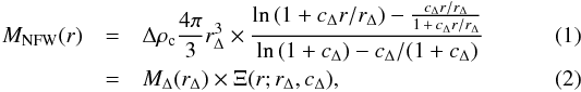$\begin{array}{ccc}{\mathit{M}}_{\mathrm{NFW}}\mathrm{\left(}\mathit{r}\mathrm{\right)}& \mathrm{=}& \mathrm{\Delta }{\mathit{\rho }}_{\mathrm{c}}\frac{\mathrm{4}\mathit{\pi }}{\mathrm{3}}{\mathit{r}}_{\mathrm{\Delta }}^{\mathrm{3}}\mathrm{\times }\frac{\ln \mathrm{(}\mathrm{1}\mathrm{+}{\mathit{c}}_{\mathrm{\Delta }}\mathit{r}\mathit{/}{\mathit{r}}_{\mathrm{\Delta }}\mathrm{)}\mathrm{-}\frac{{\mathit{c}}_{\mathrm{\Delta }}\mathit{r}\mathit{/}{\mathit{r}}_{\mathrm{\Delta }}}{\mathrm{1}\hspace{0.17em}\mathrm{+}\hspace{0.17em}{\mathit{c}}_{\mathrm{\Delta }}\mathit{r}\mathit{/}{\mathit{r}}_{\mathrm{\Delta }}}}{\ln \mathrm{(}\mathrm{1}\mathrm{+}{\mathit{c}}_{\mathrm{\Delta }}\mathrm{)}\mathrm{-}{\mathit{c}}_{\mathrm{\Delta }}\mathit{/}\mathrm{(}\mathrm{1}\mathrm{+}{\mathit{c}}_{\mathrm{\Delta }}\mathrm{)}}\\ & \mathrm{=}& {\mathit{M}}_{\mathrm{\Delta }}\mathrm{\left(}{\mathit{r}}_{\mathrm{\Delta }}\mathrm{\right)}\mathrm{\times }\mathrm{\Xi }\mathrm{\left(}\mathit{r}\mathrm{;}{\mathit{r}}_{\mathrm{\Delta }}\mathit{,}{\mathit{c}}_{\mathrm{\Delta }}\mathrm{\right)}\mathit{,}\end{array}$separating into the mass M_Δ and a function we call Ξ(r;r_Δ,c_Δ). Equating Eq. (1) with r = r₅₀₀ for Δ = 200 and Δ′ = 500, we arrive at this implicit equation for r₅₀₀, which we solve numerically: $\begin{array}{ccc}{\mathit{r}}_{\mathrm{500}}\mathrm{=}{\mathit{r}}_{\mathrm{200}}{\mathrm{(}\frac{\mathrm{2}}{\mathrm{5}}\hspace{0.17em}\mathrm{\Xi }\mathrm{(}{\mathit{r}}_{\mathrm{500}}\mathit{,}{\mathit{r}}_{\mathrm{200}}\mathit{,}{\mathit{c}}_{\mathrm{200}}{\mathrm{)}}^{\mathrm{)}}}^{\mathrm{1}\mathit{/}\mathrm{3}}\mathit{.}& & \end{array}$(3)

2.4. X-ray analysis

Under the strong assumptions that the ICM is in hydrostatic equilibrium and follows a spherically symmetric mass distribution, the cluster mass within a radius r can be calculated as (see e.g. Sarazin 1988): $\begin{array}{ccc}{\mathit{M}}^{\mathrm{hyd}}\mathrm{\left(}\mathit{r}\mathrm{\right)}\mathrm{=}\frac{\mathrm{-}{\mathit{k}}_{\mathrm{B}}{\mathit{T}}_{\mathrm{X}}\mathrm{\left(}\mathit{r}\mathrm{\right)}\hspace{0.17em}\mathit{r}}{\mathit{\mu }{\mathit{m}}_{\mathrm{p}}\mathit{G}}\left(\frac{\mathrm{d}\ln {\mathit{\rho }}_{\mathrm{g}}\mathrm{\left(}\mathit{r}\mathrm{\right)}}{\mathrm{d}\ln \mathit{r}}\mathrm{+}\frac{\mathrm{d}\ln {\mathit{T}}_{\mathrm{X}}\mathrm{\left(}\mathit{r}\mathrm{\right)}}{\mathrm{d}\ln \mathit{r}}\right)& & \end{array}$(4)from the ICM density and temperature profiles ρ_g(r) and T_X(r), where G is the gravitational constant, m_p is the proton mass, and μ = 0.5954 the mean molecular mass of the ICM. The ICM density is modelled by fitting the observed Chandra surface brightness profile, assuming a primordial He abundance and an ICM metallicity of 0.2 Z_⊙, such that ρ_g(r) = 1.274 m_pn(r). We use a Vikhlinin et al. (2006) particle density profile with $\mathit{n}\mathrm{\left(}\mathit{r}\mathrm{\right)}\mathrm{=}\sqrt{{\mathit{n}}_{\mathrm{p}}\mathrm{\left(}\mathit{r}\mathrm{\right)}\hspace{0.17em}{\mathit{n}}_{\mathrm{e}}\mathrm{\left(}\mathit{r}\mathrm{\right)}}$. Extending the widely-used β-profile (Cavaliere & Fusco-Femiano 1978), it allows for prominent cluster cores as well as steeper surface brightness profiles in the cluster outskirts to be modelled by additional terms. Regarding the systematic differences Rozo et al. (2014b) find between X-ray mass algorithms, we point out that we employ the V09a profiles directly rather than re-deriving them from their parameters.

The relatively low signal/noise in the Chandra data renders the determination of individual temperature profiles difficult. Rather, we fit a global T_X (Table 1; V09a) and assume the empirical average temperature profile T_X(r) = T_X⁽1.19 − 0.84r/r₂₀₀⁾Reiprich et al. (2013) derive from compiling all available Suzaku temperature profiles (barring only the two most exceptional clusters). For r₂₀₀, we use the WL results from Paper II².

Equation (4) provides us with a cumulative mass profile. We evaluate this profile at some r_test, e.g. from WL, and propagate the uncertainty in r_test, together with the uncertainty in T_X.

Hydrostatic equilibrium and sphericity are known to be problematic assumptions for many clusters. Nonetheless, hydrostatic masses are commonly used in the literature in comparisons to WL masses. Our goal is to study if and how biases due to deviations from the above-mentioned assumptions show up.

2.5. Mass estimates

Table 1 comprises the key results on radii r₅₀₀ and the corresponding mass estimates. By , we denote a mass measured from data on proxy within a radius defined by proxy . We use five mass estimates: . The first two are the weak lensing (wl) and hydrostatic X-ray masses (hyd), as introduced in Sects. 2.2 and 2.4. Having analysed deep Chandra observations they acquired, Vikhlinin et al. (2009a) present three further mass estimates for all 36 clusters in the complete sample. Based on the proxies T_X, the ICM mass M_gas, and Y_X = T_XM_gas, mass estimates M^T, M^G, and M^Y are quoted in Table 2 of V09a. We point out that V09a obtain these estimates by calibrating the mass scaling relations for respective proxy on local clusters (see their Table 3). V09a further provide a detailed account of the relevant systematic sources of uncertainty.

The radii ${\mathit{r}}_{\mathrm{500}}^{\mathrm{𝒫}}\mathrm{=}{{}^{\mathrm{(}}\mathrm{3}{\mathit{M}}_{\mathrm{500}}^{\mathrm{𝒫}}\mathit{/}\mathrm{(}\mathrm{2000}\mathit{\pi }{\mathit{\rho }}_{\mathrm{c}}{\mathrm{\left)}}^{\mathrm{\right)}}}^{\mathrm{1}\mathit{/}\mathrm{3}}$ listed in Table 1 are obtained from ${\mathit{M}}_{\mathrm{500}}^{\mathrm{𝒫}}\mathit{,}\hspace{0.17em}\mathrm{𝒫}\mathrm{\in }\mathrm{\left\{}\mathrm{Y}\mathit{,}\mathrm{T}\mathit{,}\mathrm{G}\mathrm{\right\}}$. Using Eqs. (1) and (4), we then derive the WL and hydrostatic masses, respectively, within these radii. We emphasise that all WL mass uncertainties quoted in Table 1 are purely statistical and do not include any of the systematics discussed in Paper II.

2.6. Fitting algorithm for scaling relations

The problem of selecting the best linear representation y = A + Bx for a sample of (astronomical) observations of two quantities { x_i } and { y_i } can be surprisingly complex. A plethora of algorithms and literature cope with the different assumptions about measurement uncertainties one can or has to make (e.g. Press et al. 1992; Akritas & Bershady 1996; Tremaine et al. 2002; Kelly 2007; Hogg et al. 2010; Williams et al. 2010; Andreon & Hurn 2012; Feigelson & Babu 2012). The challenges observational astronomers have to tackle when trying to reconcile the prerequisites of statistical estimators with the realities of astrophysical data are manifold, including heteroscedastic uncertainties (i.e. depending non-trivially on the data themselves), intrinsic scatter, poor knowledge of systematics, poor sample statistics, “outlier” points, and non-Gaussian probability distributions. Tailored to the problem of galaxy cluster scaling relations, Maughan (2014) proposed a “self-consistent” modelling approach based on the fundamental observables. A full account of these different effects exceeds the scope of this article. We choose the relatively simple fitexy algorithm (Press et al. 1992), minimising the estimator $\begin{array}{ccc}{\mathit{\chi }}_{\mathrm{P}\mathrm{92}}^{\mathrm{2}}\mathrm{=}\sum _{\mathit{i}\mathrm{=}\mathrm{1}}^{\mathit{N}}\frac{{\left({\mathit{y}}_{\mathit{i}}\mathrm{-}\mathit{A}\mathrm{-}\mathit{B}{\mathit{x}}_{\mathit{i}}\right)}^{\mathrm{2}}}{{\mathit{\sigma }}_{\mathit{y,i}}^{\mathrm{2}}\mathrm{+}{\mathit{B}}^{\mathrm{2}}{\mathit{\sigma }}_{\mathit{x,i}}^{\mathrm{2}}}\mathit{,}& & \end{array}$(5)which allows the uncertainties σ_x,i and σ_y,i to vary for different data points x_i and y_i, but assumes them to be drawn from a Gaussian distribution. To accommodate intrinsic scatter, ${\mathit{\sigma }}_{\mathit{y,i}}^{\mathrm{2}}$ in Eq. (5) can be replaced by ${\mathit{\sigma }}_{\mathit{i}}^{\mathrm{2}}\mathrm{=}{\mathit{\sigma }}_{\mathit{y,i}}^{\mathrm{2}}\mathrm{+}{\mathit{\sigma }}_{\mathrm{int}}^{\mathrm{2}}$ (e.g. Weiner et al. 2006; Andreon & Hurn 2012). We test for intrinsic scatter using mpfitexy (Markwardt 2009; Williams et al. 2010), but in most cases, due to the small χ² values, find the respective parameter not invoked. Thus we decide against this additional complexity. A strength of Eq. (5) is its invariance under changing x and y (e.g. Tremaine et al. 2002); i.e., we do not assume either to be “the independent variable”.

Fig. 1 Scaling of weak lensing masses ${\mathit{M}}_{\mathrm{500}}^{\mathrm{wl}}\mathrm{\left(}{\mathit{r}}_{\mathrm{500}}^{\mathrm{wl}}\mathrm{\right)}$ with hydrostatic masses ${\mathit{M}}_{\mathrm{500}}^{\mathrm{hyd}}\mathrm{\left(}{\mathit{r}}_{\mathrm{500}}^{\mathrm{wl}}\mathrm{\right)}$. The upper (lower) panel is for cfit (cB13). Both show best fits for three cases: the default (filled, thick ring, dotted ring symbols; thick dashed line), regular shear profile clusters only (filled and thick ring symbols; dash-dotted line; Sect. 4.1), and without correction for dilution by cluster members (filled, thin ring, dotted ring symbols; long dashed line; Sect. 4.3). The dotted line shows equality of the two masses, ${\mathit{M}}_{\mathrm{500}}^{\mathrm{wl}}\mathrm{=}{\mathit{M}}_{\mathrm{500}}^{\mathrm{hyd}}$. Shaded regions indicate the uncertainty range of the default best-fit. Some error bars were omitted for sake of clarity.

Rather than propagating the (unknown) distribution functions in the mass uncertainties³, we approximate 1σ Gaussian uncertainties in decadic log-space, applying the symmetrisation: $\begin{array}{ccc}{\mathit{\sigma }}_{\mathrm{\left(}\log {\mathit{\xi }}_{\mathit{i}}\mathrm{\right)}}\mathrm{=}\log \mathrm{\left(}\mathrm{e}\mathrm{\right)}\mathrm{(}{\mathit{\xi }}_{\mathit{i}}^{\mathrm{+}}\mathrm{-}{\mathit{\xi }}_{\mathit{i}}^{\mathrm{-}}\mathrm{)}\mathit{/}\mathrm{\left(}\mathrm{2}{\mathit{\xi }}_{\mathit{i}}\mathrm{\right)}\mathrm{=}\log \mathrm{\left(}\mathrm{e}\mathrm{\right)}\mathrm{(}{\mathit{\sigma }}_{\mathit{\xi ,i}}^{\mathrm{+}}\mathrm{+}{\mathit{\sigma }}_{\mathit{\xi ,i}}^{\mathrm{-}}\mathrm{)}\mathit{/}\mathrm{\left(}\mathrm{2}{\mathit{\xi }}_{\mathit{i}}\mathrm{\right)}\mathit{,}& & \end{array}$(6)where ${\mathit{\xi }}_{\mathit{i}}^{\mathrm{+}}\mathrm{=}{\mathit{\xi }}_{\mathit{i}}\mathrm{+}{\mathit{\sigma }}_{\mathit{\xi ,i}}^{\mathrm{+}}$ and ${\mathit{\xi }}_{\mathit{i}}^{\mathrm{-}}\mathrm{=}{\mathit{\xi }}_{\mathit{i}}\mathrm{-}{\mathit{\sigma }}_{\mathit{\xi ,i}}^{\mathrm{-}}$ are the upper and lower limits of the 1σ interval (in linear space) for the datum ξ_i, given the uncertainties ${\mathit{\sigma }}_{\mathit{\xi ,i}}^{\mathrm{\pm }}$. All our calculations and plots use { x_i } : = { log ξ_i } and { σ_x,i } : = { σ_(log ξi) }, with log ≡ log ₁₀.

3. Results

3.1. Weak lensing and hydrostatic masses

Fig. 2 Ratios between X-ray and WL masses as a function of WL mass. Panel A) shows log (Mhyd/Mwl) within ${\mathit{r}}_{\mathrm{500}}^{\mathrm{wl}}$, panel B) shows log (MY/Mwl) within ${\mathit{r}}_{\mathrm{500}}^{\mathrm{Y}}$. WL masses assume the B13 c–M relation. We show three tests for a mass bias: the overall average logarithmic bias b = ⟨ log MX − log Mwl ⟩ is denoted by a long-dashed line, and its standard error by a dark grey shading. Short-dashed lines and light grey shading denote the same quantity, but obtained from averaging over Monte Carlo realisations including the jackknife test. We also show this bMC for the low-Mwl and high-Mwl clusters separately, with the 1σ uncertainties presented as boxes, for sake of clarity. As a visual aid, a dot-dashed line depicts the Monte Carlo/jackknife best-fit of log (MX/Mwl) as a function of Mwl. In addition, panel A) also contains this best-fit line (triple-dot-dashed) for the case without correction for cluster member dilution; the corresponding data points follow the Fig. 1 scheme. Indicated by uncertainty bars, panel B) also presents three high-z clusters from High et al. (2012).

The first and single most important observation is that hydrostatic masses ${\mathit{M}}_{\mathrm{500}}^{\mathrm{hyd}}\mathrm{\left(}{\mathit{r}}_{\mathrm{500}}^{\mathrm{wl}}\mathrm{\right)}$, i.e. evaluated at r₅₀₀ as found from weak lensing, and weak lensing masses ${\mathit{M}}_{\mathrm{500}}^{\mathrm{wl}}\mathrm{\left(}{\mathit{r}}_{\mathrm{500}}^{\mathrm{wl}}\mathrm{\right)}$ roughly agree with each other (Table 1). Our second key observation is the very tight scaling behaviour between ${\mathit{M}}_{\mathrm{500}}^{\mathrm{hyd}}$ and ${\mathit{M}}_{\mathrm{500}}^{\mathrm{wl}}$, as Fig. 1 shows. In all cases presented in Fig. 1, and most of the ones we tested, all data points are consistent with the best-fit relation. Consequently, the fits return small values of ${\mathit{\chi }}_{\mathrm{red}}^{\mathrm{2}}\mathit{<}\mathrm{1}$ (see Table 2). Bearing in mind that we only use stochastic uncertainties, this points to some intrinsic correlation of the WL and hydrostatic masses. We will discuss this point in Sect. 4.2.

Finally, we find the slope of the ${\mathit{M}}_{\mathrm{500}}^{\mathrm{wl}}\mathrm{\left(}{\mathit{r}}_{\mathrm{500}}^{\mathrm{wl}}\mathrm{\right)}$–${\mathit{M}}_{\mathrm{500}}^{\mathrm{hyd}}\mathrm{\left(}{\mathit{r}}_{\mathrm{500}}^{\mathrm{wl}}\mathrm{\right)}$ relation (dashed lines in Fig. 1) to be steeper than unity (dotted line): using the “default model”, i.e. the analysis described in Sect. 2, a fitexy fit yields 1.71 ± 0.64 for the “c_fit” case (concentration parameters from the shear profile fits, cf. Paper II; upper panel of Fig. 1), and 1.46 ± 0.57, if the B13 mass-concentration relation is applied (“c_B13”; lower panel). The different slopes in the c_fit and c_B13 cases are mainly due to the two clusters, CL 1641+4001 and CL 1701+6414, in which the weak lensing analysis revealed shallow tangential shear profiles due to extended surface mass plateaus (cf. Figs. 3 and 5 of Paper II). This will be the starting point for further analysis and interpretation in Sect. 4.1.

Although the c_B13 slope is consistent with the expected 1:1 relation, such a ${\mathit{M}}_{\mathrm{500}}^{\mathrm{wl}}$–${\mathit{M}}_{\mathrm{500}}^{\mathrm{hyd}}$ relation would translate to extreme biases between X-ray and WL masses if extrapolated to higher and lower masses. Especially for masses of a few 10¹⁵M_⊙, ample observations disagree with the extrapolated M^wl> 2M^hyd. We do not claim our data to have such predicting power outside its mass range. Rather, we focus on what can be learnt about the X-ray/WL mass bias in our 0.4 ~ z ~ 0.5 mass range, which we, for the first time, study in the mass range down to ~1 × 10¹⁴M_⊙.

We are using three methods to test for the biases between X-ray and WL masses. First, we compute the logarithmic bias b = ⟨ log ξ − log η ⟩, which we define as the average logarithmic difference between two general quantities ξ and η. Its interpretation is that 10^bη is the average value corresponding to ξ. The uncertainty in b is given by the standard error of (log ξ − log η). Hence, our measurement of b = − 0.02 ± 0.04 for c_B13 corresponds to a vanishing fractional bias of ⟨ M^hyd ⟩ ≈ (0.97 ± 0.09) ⟨ M^wl ⟩.

Given the small sample size, large uncertainties, and the tight scaling relations in Fig. 1 pointing to some correlation between the WL and X-ray masses, we base our further tests on a Monte Carlo (MC) analysis including the jackknife test. For 10⁵ realisations, we chose with random δξ_i,k drawn from zero-mean distributions assembled from two Gaussian halves with variances ${\mathit{\sigma }}_{\mathit{\xi ,i}}^{\mathrm{-}}$ for the negative and ${\mathit{\sigma }}_{\mathit{\xi ,i}}^{\mathrm{+}}$ for the positive half⁴. This provides a simple way of accommodating asymmetric uncertainties (cf. Paper II and Table 1). Then we take the logarithm and again symmetrise the errors. We repeat for . On top, for each realisation , we discard one cluster after another, yielding a total of 8 × 10⁵ samples.

Based on those MC/jackknife realisations, we compute our second bias estimator . In order to achieve the best possible robustness against large uncertainties and small cluster numbers, we quote the ensemble median and dispersion. We find ${\mathit{b}}_{\mathrm{MC}}\mathrm{=}\mathrm{0.0}{\mathrm{0}}_{-0.13}^{\mathrm{+}\mathrm{0.14}}$ for c_B13, in good agreement with b = − 0.02 ± 0.04, i.e. a median WL/X-ray mass ratio of 1.

Fitting log (M^X/M^wl) as a function of M^wl and averaging over the MC/jackknife samples, we obtain our third bias estimator, an intercept A at the pivot mass of $\log {}^{\mathrm{(}}\mathit{M}_{\mathrm{piv}}\mathit{/}\mathrm{M}{{}_{\mathrm{\odot }}}^{\mathrm{)}}\mathrm{=}\mathrm{14.5}$. We find $\mathit{A}\mathrm{=}\mathrm{-}\mathrm{0.0}{\mathrm{2}}_{-0.08}^{\mathrm{+}\mathrm{0.07}}$ for c_B13, again consistent with vanishing bias.

3.2. Lensing masses and X-ray masses from proxies

Figures 2 and A.2, as well as Table 2 present the three different X-ray/WL mass bias estimates for four X-ray mass observables: ${\mathit{M}}_{\mathrm{500}}^{\mathrm{hyd}}$ using c_B13 from Sect. 3.1 in Panel A of Fig. 2, ${\mathit{M}}_{\mathrm{500}}^{\mathrm{Y}}$ in Panel B of Fig. 2, ${\mathit{M}}_{\mathrm{500}}^{\mathrm{T}}$ in Panel A of Fig. A.2, ${\mathit{M}}_{\mathrm{500}}^{\mathrm{G}}$ in Panel B of Fig. A.2. The last three are the proxy-based Vikhlinin et al. (2009a) X-ray mass estimators defined in Sect. 2.5. While Panel A uses ${\mathit{r}}_{\mathrm{500}}^{\mathrm{wl}}$, the other three panel use the respective ${\mathit{r}}_{\mathrm{500}}^{\mathrm{Y}\mathit{,}\mathrm{T}\mathit{,}\mathrm{G}}$.

Long-dashed lines and dark-grey boxes in Fig. 2 display b and its error. Short-dashed lines and light-grey boxes denote b_MC. The intercept A is located at the intersection of the dot-dashed fit and dotted zero lines. We also show b_MC for the low-mass and high-mass clusters separately, splitting at M^wlE(z) = M_piv; the respective 1σ ranges are shown as outline boxes.

We observe remarkable agreement between the X-ray/WL mass ratios and bias fits from all four X-ray observables (which are not fully independent). For each of them, all three bias estimates agree with each other, and all are consistent with no X-ray/WL mass bias. We find no evidence for X-ray masses being biased low by ~40% in our cluster sample, as it has been suggested to explain the Planck CMB – SZ cluster counts discrepancy. While b_MC ≥ 0.2 (≳35% mass bias) lies within the possible range of the high-M^wl bin, in particular using the gas mass M^G, the overall cluster sample does not support this hypothesis. We point out that b_MC was designed to be both robust against possible effects of large uncertainties and the small number of clusters in this first batch of 400d WL clusters. The larger uncertainties in b_MC compared to b are directly caused by the jackknife test and the account for possible fit instability in the MC method.

The slopes B quantifying the M^wl dependence of the X-ray/WL mass ratio are significantly negative in all of our measurements. This directly corresponds to the steep slope in the mass-mass scaling (Fig. 1). Predicting cluster masses for very massive clusters (or low-mass groups) from B = − 0.75 for M^Y would yield M^X = M^wl/ 2 at 10¹⁵ M_⊙/E(z) (and M^X = 2.8 M^wl at 10¹⁴M_⊙/E(z)). Such ratios are at odds with existing measurements. Therefore, we refrain from extrapolating cluster masses, but interpret the slopes B as indicative of a possibly mass-dependent X-ray/WL mass ratio. This evidence is more prudently presented as the ~2σ discrepancy between the low-M^wl and high-M^wl mass bins for all three V09a X-ray observables.

4. A mass-dependent bias?

In this section, we analyse two unexpected outcomes of our study in greater detail: the clear correlation between the M^X/M^wl measurement of the individual clusters and their lensing masses, and the unusually small scatter in our scaling relations. Results for ancillary scaling relations that we present in Appendix A underpin the findings of Fig. 1 and Table 2. To begin with, we emphasise that the mass-dependent bias is not caused by the conflation of a large z range; all but one of our clusters inhabit the range 0.39 ≤ z ≤ 0.53 across which E(z) varies by <10%, and we accounted for this variation. As Fig. A.2 shows, this also leaves us with little constraining power with regard to a z-dependent bias, at least until the 400d WL survey becomes more complete.

4.1. Role of c₂₀₀ and departures from NFW profile

Figure 1 shows that the M^wl–M^X scaling relation sensitively depends on the choice for the cluster concentration parameter c₂₀₀. This translates into more positive bias estimates for c_fit as compared to c_B13 (Table 2). The difference is caused by the two flat-profile clusters for which NFW fits yield low masses but do not capture all the large-scale mass distribution, in particular if c₂₀₀ is determined directly from the data, rather than assuming a mass-concentration relation (cf. the discussion of the concentration parameter in Paper II and Foëx et al. 2012). This induces a bias towards low masses in the r₂₀₀ → r₅₀₀ conversion. If these two “irregular” clusters (dotted ring symbols in Fig. 1) are excluded, the “regular clusters only” M^wl–M^X scaling relations (dash-dotted lines) differ for the c_fit, but not for the c_B13 case. Moreover, their mass ratios are consistent with the other high-M^wl clusters for c_B13. We thus confirm that assuming a mass-concentration relation and marginalising over c₂₀₀ is advantageous for scaling relations. We note that Comerford et al. (2010) observed a correlation between the scatters in the mass-concentration and mass-temperature relations and advocated the inclusion of unrelaxed clusters in scaling relation studies.

Because NFW profile fits do not capture the complete projected mass morphologies of irregular clusters, the assumption of that profile for ${\mathit{M}}_{\mathrm{500}}^{\mathrm{wl}}\mathrm{\left(}{\mathit{r}}_{\mathrm{500}}^{\mathrm{wl}}\mathrm{\right)}$ (Eq. 3), and ${\mathit{M}}_{\mathrm{500}}^{\mathrm{wl}}\mathrm{\left(}{\mathit{r}}_{\mathrm{500}}^{\mathrm{Y}}\mathrm{\right)}$, etc. (Sect. 3.2) could introduce a further bias. Aperture-based lensing masses, e.g. the ζ_c statistics (Clowe et al. 1998) employed by Hoekstra et al. (2012) provide an alternative. However, Okabe et al. (2013) demonstrated by the stacking of 50 clusters from the Local Cluster Substructure Survey (0.15 <z< 0.3), that the average weak lensing profile does follow NFW to a high degree, at least at low redshift. Furthermore, the Planck Collaboration (2013) finds a trend of M^wl/M^hyd with the ratio of concentration parameters measured from weak lensing and X-rays.

4.2. Correlation between mass estimates

In Table 2, we quote ${\mathit{\chi }}_{\mathrm{red}}^{\mathrm{2}}$ for the M^wl–M^X scaling relations, using the same MC/jackknife samples as for the bias tests. For the ones involving hydrostatic masses, we measure $\mathrm{0.5}\mathit{<}{\mathit{\chi }}_{\mathrm{red}}^{\mathrm{2}}\mathit{<}\mathrm{0.6}$. We evaluated ${\mathit{M}}_{\mathrm{500}}^{\mathrm{hyd}}$ at ${\mathit{r}}_{\mathrm{500}}^{\mathrm{wl}}$ in order to measure both estimates within the same physical radius, in an “apples with apples” comparison. But using the lensing-derived radius also introduces an unknown amount of correlation, a possible (partial) cause of the measured low ${\mathit{\chi }}_{\mathrm{red}}^{\mathrm{2}}$ values.

We test for the impact of the correlation by measuring both M^wl and M^hyd within a fixed physical radius for all clusters, and choose r_fix = 800 kpc as a rough sample average of r₅₀₀. Surprisingly, we find an only slightly higher ${\mathit{\chi }}_{\mathrm{red}}^{\mathrm{2}}$, still <1 (see Table 2). As before, the bias estimators are consistent with zero. Fixed radii of 600 kpc and 1000 kpc give similar results (Table 2 and Fig. A.2). with a tentative trend of increasing ${\mathit{\chi }}_{\mathrm{red}}^{\mathrm{2}}$ with smaller radii. Interestingly, a low ${\mathit{\chi }}_{\mathrm{red}}^{\mathrm{2}}$ is also found for the M^wl–M^T and M^T–M^hyd relations (Table A.2). The latter is expected, because M^hyd are derived from the same T_X and depend sensitively on them. This all suggests that the small scatter is not driven by using ${\mathit{r}}_{\mathrm{500}}^{\mathrm{wl}}$, but by some other intrinsic factor.

If the uncertainties in M^wl were overestimated significantly, this would obviously explain the low ${\mathit{\chi }}_{\mathrm{red}}^{\mathrm{2}}$. However, we do not even include systematic effects here. Moreover, the quoted M^wl uncertainties directly come from the NFW modelling of Paper II and reflect the Δχ² from their Eq. (3), given the shear catalogue. The errors are dominated by the intrinsic source ellipticity σ_ε, for which we, after shear calibration, find values of ~0.3, consistent with other ground-based WL experiments. Therefore, despite the allure of our WL errors being overestimated, we do not find evidence for this hypothesis in our shear catalogues. Furthermore, the quoted M^wl uncertainties are consistent with the aperture mass detection significances we reported in Paper II.

4.3. Dilution by cluster members and foregrounds

Comparing the complete set of mass-mass scaling relations our data offer (Table A.2), we trace the mass-dependence of the bias seen in Fig. 2 back to the different ranges spanned by the estimates for r₅₀₀. While the ratio of minimum to maximum is ≈0.75 for ${\mathit{r}}_{\mathrm{500}}^{\mathrm{Y}}$, ${\mathit{r}}_{\mathrm{500}}^{\mathrm{T}}$, and ${\mathit{r}}_{\mathrm{500}}^{\mathrm{hyd}}$, the same ratio is 0.57 for ${\mathit{r}}_{\mathrm{500}}^{\mathrm{wl}}$, using the B13 M–c relation. In the following, we discuss the potential influence of several sources of uncertainty in the WL masses, showing that the dispersion between lowest and highest ${\mathit{M}}_{\mathrm{500}}^{\mathrm{wl}}$ is likely an inherent feature rather than a modelling artefact.

In Paper II, we discussed the great effort we took in constructing the best-possible homogeneous analysis from the quite heterogeneous MMT imaging data. Unfortunately, we happen to find higher M^wl for all clusters with imaging in three bands than for the clusters with imaging in one band. We emphasise there are no trends with limiting magnitude, seeing, or density n_KSB of galaxies with measurable shape (cf. Tables 1 and 2 in Paper II).

In the cases where three-band imaging is available, our WL model includes a correction for the diluting effect residual cluster member galaxies impose on the shear catalogue. For the other clusters, no such dilution correction could be applied. A rough estimate of the fraction of unlensed galaxies remaining after background selection suggests that the contamination in single-band catalogues is ~30–50% higher than with the more sophisticated galaxy-colour based method. Therefore, we re-calculate the scaling relations, switching off the dilution correction (long dashed line and thin ring symbols in Fig. 1). This lowers the r₅₀₀ values by ~6% and the masses by 10–15%. For both the ${\mathit{M}}_{\mathrm{500}}^{\mathrm{wl}}$–${\mathit{M}}_{\mathrm{500}}^{\mathrm{hyd}}$ and ${\mathit{M}}_{\mathrm{500}}^{\mathrm{wl}}$–${\mathit{M}}_{\mathrm{500}}^{\mathrm{Y}}$ relations, we only observe a slightly smaller difference between b_MC for the high- and low-M^wl bins (Tables 2 and A.2), not significant given the uncertainty margins.

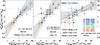Fig. 3 Comparisons with literature data. Left panel: black symbols show z> 0.35 clusters from Mahdavi et al. (2013), whose best-fit using Eq. (5) is shown by the dot-dashed line. The cluster CL 1524+0957 is indicated by a diamond symbol. Coloured symbols and the dashed line show the “default” ${\mathit{M}}_{\mathrm{500}}^{\mathrm{wl}}$–${\mathit{M}}_{\mathrm{500}}^{\mathrm{hyd}}$ relation for cB13 as in the lower panel of Fig. 1. Middle panel: the same, but comparing to Foëx et al. (2012) (black symbols and dot-dashed line for best fit). X-ray masses are measured within ${\mathit{r}}_{\mathrm{500}}^{\mathrm{hyd}}$. CL 1003+3253 and CL 1120+4318 are emphasised by special symbols. Right panel: scaling of lensing masses ${\mathit{M}}_{\mathrm{500}}^{\mathrm{wl}}$ with the YX proxy. Black symbols show the z> 0.35 clusters from M13, to which the thick, dash-dotted line is the best fit. Shaded regions indicate the uncertainties to this fit. The thin, dash-dotted line gives the best fit M13 quote for their complete sample, while the thin solid and long-dashed lines mark the M500–YX relations by V09a and Arnaud et al. (2010), respectively, for z = 0.40.

The dilution of the shear signal by an increased number of galaxies not bearing a shear signal can also be expressed as a overestimation of the mean lensing depth ⟨ β ⟩. We model a possible lensing depth bias by simultaneously adding the uncertainty σ( ⟨ β ⟩) for the three-band clusters and subtracting it for the single-band ones, maximising the leveraging effect on the masses. Similar to the previous experiment⁵ we still observe a mass-dependent bias, with little change to the default model.

We further tested alternative choices of cluster centre and fitting range, but do not observe significant changes to the mass dependent-bias or to ${\mathit{\chi }}_{\mathrm{red}}^{\mathrm{2}}$ (see Appendix A.3). Although ⟨ β ⟩ is calculated for all clusters from the same catalogues, related systematics would affect the mass normalisation, but not the relative stochastic uncertainties, which determine ${\mathit{\chi }}_{\mathrm{red}}^{\mathrm{2}}$. As we consider a drastic overestimation of the purely statistic uncertainties in the WL modelling being unlikely (Sect. 4.2), the cause of the low ${\mathit{\chi }}_{\mathrm{red}}^{\mathrm{2}}$ values remains elusive. If a WL analysis effect is responsible for one or both anomalies, it has to be of a more subtle nature than the choices investigated here.

4.4. A statistical fluke?

We summarise that the ${\mathit{M}}_{\mathrm{500}}^{\mathrm{wl}}$–${\mathit{M}}_{\mathrm{500}}^{\mathrm{hyd}}$ scaling relations we observe show an unusual lack of scatter and that we find a ~2σ difference between the X-ray/WL mass ratios of our high- and low-M^wl clusters. The latter effect can be traced back to the considerable span in cluster lensing signal, which is only partly due to different background selection procedures and the dilution correction that was only applied for clusters imaged in three bands.

The question then arises if the mass-dependent bias is caused by an unlucky selection of the 8 MMT clusters from V09’s wider sample of 36. The 8 clusters were chosen to be observed first merely because of convenient telescope scheduling, and appear typical of the larger sample in terms of redshift and X-ray observables. The MMT clusters trace well the mass range and dispersion spanned by all 36 clusters in their ${\mathit{M}}_{\mathrm{500}}^{\mathrm{Y}}$–${\mathit{M}}_{\mathrm{500}}^{\mathrm{T}}$ relation. We observe the expected vanishing slopes for log (M^T/M^Y) as a function of M^Y, both for the 8 MMT clusters and for the complete sample of 36 (Table A.2).

In Table 2, we observe significant scatter (${\mathit{\chi }}_{\mathrm{red}}^{\mathrm{2}}\mathrm{=}\mathrm{2.11}$) in the ${\mathit{M}}_{\mathrm{500}}^{\mathrm{wl}}$–${\mathit{M}}_{\mathrm{500}}^{\mathrm{G}}$ relation, while Okabe et al. (2010b) and M 13 reported particularly low scatter in M^G, comparing to WL masses. This large intrinsic scatter seems to be a feature of the overall 400d sample: plotting M^G versus the two other V09 X-ray masses of all 36 clusters, we also find ${\mathit{\chi }}_{\mathrm{red}}^{\mathrm{2}}\mathit{>}\mathrm{2}$ (Table A.2), as well as significant non-zero logarithmic biases. While tracing the cause of this observation is beyond the scope of this article, it deserves further study. Because two of the clusters with highest $\left|{\mathit{M}}_{\mathrm{500}}^{\mathrm{Y}\mathit{,}\mathrm{T}}\mathrm{-}{\mathit{M}}_{\mathrm{500}}^{\mathrm{G}}\right|$ are covered by our MMT subsample, we observe a more mass-dependent M^G/M^Y,T ratio than for all 36. Overall, however, the MMT subsample is not a very biased selection.

4.5. Physical causes

An alternative and likely explanation for the mass-dependent bias we observe could be a high rate of unrelaxed clusters, especially for our least massive objects. If the departure from hydrostatic equilibrium were stronger among the low-mass clusters than for the massive ones, this would manifest in mass ratios similar to our results. Simulations show the offset from hydrostatic equilibrium to be mass-dependent (Rasia et al. 2012), despite currently being focused on the high-mass regime. Variability in the non-thermal pressure support with mass (Laganá et al. 2013) may be exacerbated by small number statistics. At high z, the expected fraction of merging clusters, especially of major mergers, increases. Unrelaxed cluster states are known to affect X-ray observables and, via the NFW fitting, also lensing mass estimates. Indeed, the two most deviant systems in Fig. 2 are CL 1416+4446 and the flat-profile “shear plateau” cluster CL 1641+4001. Although the first shows an inconspicuous shear profile, we suspect it to be part of a possibly interacting supercluster, based on the presence of two nearby structures at the same redshift, detected in X-ray as well as in our lensing maps (Paper II). Both these clusters are classified as non-mergers in the recent Nurgaliev et al. (2013) study, introducing a new substructure estimator based on X-ray morphology. However, WL and X-ray methods are sensitive to substructure on different radial and mass scales, such that this explanation cannot be ruled out. We summarise that the greater dynamical range in WL than in X-ray masses might be linked to different sensitivities of the respective methods to substructure and mergers in the low-mass, high-z cluster population we are probing, but which is currently still underexplored.

5. Comparison with previous works

5.1. The M$\begin{array}{c}\mathrm{wl}\\ \mathrm{500}\end{array}$–M$\begin{array}{c}\mathrm{hyd}\\ \mathrm{500}\end{array}$ relation

Comparison with Mahdavi et al. (2013) results:

recently, M13 published scaling relations observed between the weak lensing and X-ray masses for a sample of 50 massive clusters, partly based on the brightest clusters from the Einstein Observatory Extended Medium Sensitivity Survey (Gioia et al. 1990). Weak lensing masses for the M13 sample have been obtained from CFHT/Megacam imaging (Hoekstra et al. 2012), while the X-ray analysis combines XMM-Newton and Chandra data. While the median redshift is z = 0.23, the distribution extends to z = 0.55, including 12 clusters at z> 0.35. Owing to their selection, these 12 clusters lie above the 400d flux and luminosity cuts, making them directly comparable to our sample.

The left panel in Fig. 3 superimposes the ${\mathit{M}}_{\mathrm{500}}^{\mathrm{wl}}$ and ${\mathit{M}}_{\mathrm{500}}^{\mathrm{hyd}}$ of the M13 high-z clusters on our results. The two samples overlap at the massive (≳5 × 10¹⁴M_⊙) end, but the 400d objects probe down to 1 × 10¹⁴M_⊙ for the first time at this z and for these scaling relations. The slopes of the scaling relations are consistent: using Eq. (5), we measure B_{M − M} = 1.13 ± 0.20 for the 12 M13 objects. A joint fit with the 400d clusters (B_{M − M} = 1.46 ± 0.57) yields B_{M − M} = 1.15 ± 0.14 and a low ${\mathit{\chi }}_{\mathrm{red}}^{\mathrm{2}}\mathrm{=}\mathrm{0.54}$, driven by our data. We note that the logarithmic bias of b = 0.10 ± 0.05 for the M13 high-z clusters corresponds to a (20 ± 10) % mass bias, consistent with both the upper range of the 400d results and expectation from the literature (e.g. Laganá et al. 2010; Rasia et al. 2012).

Calculating the Hogg et al. (2010, H10) likelihood which Mahdavi et al. (2013) use, we find ${\mathit{B}}_{\mathrm{H}\mathrm{10}}\mathrm{=}\mathrm{1.1}{\mathrm{8}}_{-0.20}^{\mathrm{+}\mathrm{0.22}}$ and intrinsic scatter σ_int consistent with zero, confirming our above results. If we, however, repeating our fits from Fig. 1 with the H10 likelihood, we obtain discrepant results which highlight the differences between the various regression algorithms (see Sect. 2.6)⁶.

CL 1524+0957 at z = 0.52 is the only cluster the 400d and M13 samples share. Denoted by a black diamond in Fig. 3, its masses from the M13 lensing and hydrostatic analyses blend in with the MMT 400d clusters. If it were included in the ${\mathit{M}}_{\mathrm{500}}^{\mathrm{wl}}$–${\mathit{M}}_{\mathrm{500}}^{\mathrm{hyd}}$ relation, it would not significantly alter the best fit, but we caution that different analysis methods have been employed, e.g. M13 reporting aperture lensing masses based on the ζ_c statistics.

Comparison with Jee et al. (2011) results:

Jee et al. (2011, J11) studied 14 very massive and distant clusters (0.83 <z< 1.46) and found their WL and hydrostatic masses ${\mathit{M}}_{\mathrm{200}}^{\mathrm{wl}}$ and ${\mathit{M}}_{\mathrm{200}}^{\mathrm{hyd}}$ to agree well, similar to our results. However, they caution that their ${\mathit{M}}_{\mathrm{200}}^{\mathrm{hyd}}$ were obtained by extrapolating a singular isothermal sphere profile. Because we doubt that the Chandra-based Vikhlinin et al. (2006) model reliably describes the ICM out to such large radii, we refrain from deriving ${\mathit{M}}_{\mathrm{200}}^{\mathrm{hyd}}$. Nevertheless, we notice that our the J11 samples not only shows similar ${\mathit{M}}_{\mathrm{200}}^{\mathrm{wl}}$ than our most massive clusters, but also contains the only two 400d clusters exceeding the redshift of CL 0230+1836, CL 0152−1357 at z = 0.83 and CL 1226+3332 at z = 0.89. Their planned re-analysis will improve the leverage of our samples at the high-z end.

Comparison with Foëx et al. (2012) results:

in the middle panel of Fig. 3, we compare our results to 11 clusters from the EXCPRES XMM-Newton sample, analysed by Foëx et al. (2012, F12) and located at a similar redshift range (0.41 ≤ z ≤ 0.61) as the bulk of our sample. Selected to be representative of the cluster population at z ≈ 0.5, these objects have been studied with XMM-Newton in X-rays and CFHT/Megacam in the optical. Foëx et al. (2012) explicitly quote hydrostatic and lensing masses within their respective radii; thus we also show the ${\mathit{M}}_{\mathrm{500}}^{\mathrm{wl}}\mathrm{\left(}{\mathit{r}}_{\mathrm{500}}^{\mathrm{wl}}\mathrm{\right)}$–${\mathit{M}}_{\mathrm{500}}^{\mathrm{hyd}}\mathrm{\left(}{\mathit{r}}_{\mathrm{500}}^{\mathrm{hyd}}\mathrm{\right)}$. Again, the more massive of our clusters resemble the F12 sources, with the 400d MMT sample extending towards lower masses. Indeed, F12 study two clusters which are part of our sample: these, CL 1002+3253 at z = 0.42 and CL 1120+4318 at z = 0.60 mark their lowest lensing mass objects. At similar ${\mathit{M}}_{\mathrm{500}}^{\mathrm{wl}}$ on either sides of the best-fit 400d scaling relation, their inclusion with the quoted masses would have no immediate effect on its slope, but slightly increase its scatter.

Bearing in mind that Fig. 3 (middle panel) compares quantities measured at different radii, we notice that the significantly flat best fit regression line to the F12 cluster masses, showing a larger dispersion in hydrostatic than in WL masses, as opposed to the 400d MMT clusters. The comparisons in Fig. 3 underscore that while being broadly compatible with each other, different studies are shaped by the fine details of their sample selection and analysis methods. We will conduct a more detailed comparison between our results and the ones of Foëx et al. (2012) and Mahdavi et al. (2013) once we re-analysed the CFHT/Megacam of the three overlapping clusters, having already shown the MMT and CFHT Megacams to produce consistent lensing catalogues (Paper II).

5.2. The ${\mathit{M}}_{\mathrm{500}}^{\mathrm{wl}}$–${\mathit{M}}_{\mathrm{500}}^{\mathrm{Y}}$ relation

The right panel of Fig. 3 investigates the scaling behaviour of ${\mathit{M}}_{\mathrm{500}}^{\mathrm{wl}}$ with Y_X by comparing the 400d MMT clusters to the z> 0.35 clusters from M13⁷. The difference between the two samples is more pronounced than in the left panel, with only the low-mass end of the M13 sample, including CL 1524+0957, overlapping with our clusters. None of the 400d MMT clusters deviates significantly from the M₅₀₀–Y_X relation applied by V09a in the derivation of the ${\mathit{M}}_{\mathrm{500}}^{\mathrm{Y}}$ masses we used. The V09a M₅₀₀–Y_X relation based on Chandra data for low-z clusters (Vikhlinin et al. 2006) is in close agreement to the M13 result for their complete sample, as well as the widely used Arnaud et al. (2010)M₅₀₀–Y_X relation. For the latter as well as V09a we show the version with a slope fixed to the self-similar expectation of B = 3 / 5. The best fit to the M13 z> 0.35 essentially yields the same slope as the complete sample (B = 0.55 ± 0.09 compared to B_H10 = 0.56 ± 0.07, calculated with the H10 method). The higher normalisation for the high-z subsample can be likely explained as Malmquist bias due to the effective higher mass limit in the M13 sample selection. The incompatibility of the least massive MMT clusters with this fit highlights that we sample lower mass clusters, which, at the same redshift, are likely to have different physical properties.

The Y_X proxy is the X-ray equivalent to the integrated pressure signal Y_SZ seen by SZ observatories. Observations confirm a close Y_X–Y_SZ correlation, with measured departures from the 1:1 slope considered inconclusive (Andersson et al. 2011; Rozo et al. 2012). Performing a cursory comparison with SZ observations, we included in Fig. 2A data for three z> 0.35 clusters from High et al. (2012) (dashed uncertainty bars), taken from their Fig. 6. The abscissa values for the High et al. (2012) clusters (SPT-CL J2022−6323, SPT-CL J2030−5638, and SPT-CL J2135−5726) show masses based on Y_SZ, derived from South Pole Telescope SZ observations (Reichardt et al. 2013). The M^wl are derived from observations with the same Megacam instrument we used for the 400d clusters, but after its transfer to the Magellan Clay telescope at Las Campanas Observatory, Chile. In good agreement with zero bias, the High et al. (2012) clusters are consistent with some of the lower mass 400d clusters. This result suggests that the Y_X–Y_SZ equivalence might hold once larger samples at high z and low masses will become available.

6. Summary and conclusions

In this article, we analysed the scaling relation between WL and X-ray masses for 8 galaxy clusters drawn from the 400d sample of X-ray-luminous 0.35 ≤ z ≤ 0.89 clusters. WL masses were measured from the Israel et al. (2012) MMT/Megacam data, and X-ray masses were based on the V09a Chandra analysis. We summarise our main results as follows:

• 1.

  We probe the WL–X-ray mass scaling relation,in an unexplored region of the parameter spacefor the first time: the z ~ 0.4–0.5 redshift range, down to1 × 10¹⁴M_⊙.

• 2.

  Using several X-ray mass estimates, we find the WL and X-ray masses to be consistent with each other. Most of our clusters are compatible with the M^X = M^wl line.

• 3.

  Assuming the M^wl not to be significantly biased, we do not find evidence for a systematic underestimation of the X-ray masses by ~40%, as suggested as a possible solution to the discrepancy between the Planck CMB constraints on Ω_m and σ₈ (the normalisation of the matter power spectrum) and the Planck SZ cluster counts (Planck Collaboration XX 2014). While our results favour a small WL-X-ray mass bias, they are consistent with both vanishing bias and the ~20% favoured by studies of non-thermal pressure support.

• 4.

  For the mass-mass scaling relations involving M^wl, we observe a surprisingly low scatter $\mathrm{0.5}\mathit{<}{\mathit{\chi }}_{\mathrm{red}}^{\mathrm{2}}\mathit{<}\mathrm{0.6}$, although we use only stochastic uncertainties and allow for correlated errors via a Monte Carlo method. Because the errors in M^wl are largely determined by the intrinsic WL shape noise σ_ε, we however deem a drastic overestimation unlikely (Sect. 4.2). For the scaling relations involving M_G, however, we observe a large scatter, contrary to Okabe et al. (2010b) and M13.

• 5.

  Looking in detail, there are intriguing indications for a mass-dependence of the WL-X-ray mass ratios of our relatively low-mass z ~ 0.4–0.5 clusters. We observe a mass bias in the low–M^wl mass bin at the ~2σ level when splitting the sample at log (M_piv/M_⊙) = 14.5 This holds for the masses V09a report based on the Y_X, T_X, and M_G proxies.

The discrepant temperatures Chandra and XMM-Newton measure in clusters (Nevalainen et al. 2010; Schellenberger et al. 2012) could provide a possible avenue to reconcile Planck cluster properties with the Planck cosmology.

We thoroughly investigate possible causes for the mass-dependent bias and tight scaling relations. First (Sect. 4.1), we confirm that by using a mass-concentration relation instead of directly fitting c₂₀₀ from WL, we already significantly reduced the bias due to conversion from r₂₀₀ to r₅₀₀. We emphasise that, on average, the NFW shear profile represents a suitable fit for the cluster population (cf. Okabe et al. 2013). Measuring M^hyd within ${\mathit{r}}_{\mathrm{500}}^{\mathrm{wl}}$ induces correlation between the data points in Fig. 1. Removing this correlation by plotting both masses within a fixed physical radius, we still find small scatter (Sect. 4.2).

We notice that the mass range occupied by the M^wl exceeds the X-ray mass ranges. Partially, this higher WL mass range can be explained by the correction for dilution by member galaxies, which could be applied only where colour information was available (Paper II). Coincidentally, this is the case for the more massive half of the MMT sample in terms of M^wl, thus boosting the range of measured WL masses (Sect. 4.3). This result underscores the importance of correcting for the unavoidable inhomogeneities in WL data due to the demanding nature of WL observations (cf. Applegate et al. 2014). We find no further indications for biases via the WL analysis. Furthermore the tight scaling precludes strong redshift effects, and we find that our small MMT subsample is largely representative of the complete sample of 36 clusters, judging from the M^Y–M^T relation (Sect. 4.4). For the M^Y–M^G and M^T–M^G relations, significant scatter (${\mathit{\chi }}_{\mathrm{red}}^{\mathrm{2}}\mathit{>}\mathrm{2}$) is present in the larger sample. The former relation also shows indications for a significant bias of M^Y ≈ 1.15M^G.

Weak lensing and hydrostatic masses for the 400d MMT clusters are in good agreement with the z> 0.35 part of the Mahdavi et al. (2013) sample and the ${\mathit{M}}_{\mathrm{500}}^{\mathrm{wl}}$–${\mathit{M}}_{\mathrm{500}}^{\mathrm{hyd}}$ relation derived from it (Sect. 5.1). The M13 and Foëx et al. (2012) samples include three 400d clusters with CFHT WL masses. These clusters neither point to significantly higher scatter nor to a less mass-dependent bias (Fig. 3). We are planning a re-analysis of the CFHT data, having demonstrated in Paper II that lensing catalogues from MMT and CFHT are nicely compatible. Such reanalysis is going to be helpful to identify more subtle WL analysis effects potentially responsible for the steep slopes and tight correlation of WL and X-ray masses.

An alternative explanation are intrinsic differences in the low-mass cluster population. That the 400d MMT sample probes to slightly lower masses (1 × 10¹⁴M_⊙) than M13 or F12 becomes especially obvious from the M^wl–Y^X relation (Fig. 3, Sect. 5.2). Because the 400d sample is more representative of the z ~ 0.4–0.5 cluster population, it is likely to contain more significant mergers relative to the cluster mass, skewing mass estimates (Sect. 4.5). Hence, the 400d survey might be the first to see the onset of a mass regime in which cluster physics and substructure lead the WL-X-ray scaling to deviate from what is known at higher masses. Remarkably, Giles et al. (2014) are finding a different steep slopes in their low-mass WL-X-ray scaling analysis. Detailed investigations of how their environment shapes clusters like CL 1416+4446 might be necessary to improve our understanding of the cluster population to be seen by future cosmology surveys. Analysis systematics might also behave differently at lower masses. A turn for WL cluster science towards lower mass objects, e.g. through the completion of the 400d WL sample, will help addressing the question of evolution in lensing mass scaling relations.

Note added in proof. After this paper was accepted, another paper (von der Linden et al. 2014b) appeared as submitted, pointing at the combined effects of hydrostatic mass bias and calibration systematics. The cross calibration effect on cosmological parameter constraints is currently being tested directly by Schellenberger et al. (in prep.). Rozo et al. (2014a,b) review and cross-calibrate the various scaling relations involved. Alternatively, Burenin (2013) suggested additional massive neutrino species.

Online material

Appendix A: Further scaling relations and tests

Fig. A.1 Lensing mass – X-ray luminosity relation. The M–LX relation is shown, for both ${\mathit{M}}_{\mathrm{500}}^{\mathrm{wl}}\mathrm{\left(}{\mathit{r}}_{\mathrm{500}}^{\mathrm{wl}}\mathrm{\right)}$ (filled circles) and ${\mathit{M}}_{\mathrm{500}}^{\mathrm{Y}}\mathrm{\left(}{\mathit{r}}_{\mathrm{500}}^{\mathrm{Y}}\mathrm{\right)}$ (small triangles). Open triangles represent the sample clusters for which MMT lensing masses are not available. The V09a M–LX relation at z = 0.40 (z = 0.80) is denoted by a long-dashed black (short-dashed red) line. Shaded (hatched) areas show the respective 1σ intrinsic scatter ranges.

Appendix A.1: The L_X–M relation

To better assess the consistency of our weak lensing masses with the Vikhlinin et al. (2009a) results, we compare them to the L_X–M_Y-relation derived by V09a using the ${\mathit{M}}_{\mathrm{500}}^{\mathrm{Y}}$ masses of their low-z cluster sample. Figure A.1 inverts this relation by showing the ${\mathit{M}}_{\mathrm{500}}^{\mathrm{wl}}\mathrm{\left(}{\mathit{r}}_{\mathrm{500}}^{\mathrm{wl}}\mathrm{\right)}$ masses as a function of the 0.5–2.0 keVChandra luminosities measured by V09a. Statistical uncertainties in the Chandra fluxes and, hence, luminosities are negligible for our purposes. We calculate the expected 68 % confidence ranges in mass for a given luminosity by inverting the scatter in L_X at a fixed M^Y as given in Eq. (22) of V09a. For two fiducial redshifts, z = 0.40 and z = 0.80, spanning the unevenly populated redshift range of the eight clusters, the M–L_X relations and their expected scatter are shown in Fig. A.1. Small filled triangles in Fig. A.1 show the ${\mathit{M}}_{\mathrm{500}}^{\mathrm{Y}}$ masses from which V09a derived the L_X–M relation. Our 8 MMT clusters are nicely tracing the distribution of the overall sample of 36 clusters (open triangles).

As an important step in the calculation of the mass function, these authors show that their procedure is able to correct for the Malmquist bias even in the presence of evolution in the L_X–M

relation, which they include in the model. We emphasise that the Malmquist bias correction – which is not included here – applied by V09a moves the clusters upwards in Fig. A.1, such that the sample agrees with the best-fit from the low-z sample, as Fig. 12 in V09a demonstrates.

As already seen in Fig. 2, the M^wl (large symbols in Fig. A.1) and M^Y agree well. Thus we can conclude that the WL masses are consistent with the expectations from their L_X. Finally, we remark that the higher X-ray luminosities for the some of the same clusters reported by Maughan et al. (2012) in their study of the L_X–T_X relation are not in disagreement with V09a, as Maughan et al. (2012) used bolometric luminosities.

Appendix A.2: Redshift scaling and cross-scaling of X-ray masses

Here we show further results mentioned in the main body of the article. Figure A.2 shows two examples of the X-ray/WL mass ratio as a function of redshift. Owing to the inhomegenous redshift coverage of our clusters, we cannot constrain a redshift evolution. All of our bias estimates are consistent with zero bias.

Table A.2 shows the fit results and bias estimates for various tests we performed modifying our default model, as well as for ancillary scaling relations. In particular, we probe the scaling behaviour of hydrostatic masses against the V09a estimates, for which we find a M^Y/M^hyd tentatively biased high by ~15%, while M^T and M^G do not show similar biases.

Appendix A.3: Choice of centre and fitting range

Weak lensing masses obtained from profile fitting have been shown to be sensitive to the choice of the fitting range (Becker & Kravtsov 2011; Hoekstra et al. 2011b; Oguri & Hamana 2011). Taking these results into account, we fitted the WL masses within a fixed physical mass range. Varying the fitting range by using r_min = 0 instead of 0.2 Mpc in one and r_max = 4.0 Mpc instead of 5.0 Mpc in another test, we find no evidence for a crucial influence on our results.

Both simulations and observations establish (e.g. Dietrich et al. 2012; George et al. 2012) that WL masses using lensing cluster centres are biased high due to random noise with respect to those based on independently obtained cluster centres, e.g. the ROSAT centres we employ. The fact that the ${\mathit{M}}_{\mathrm{500}}^{\mathrm{wl}}$–${\mathit{M}}_{\mathrm{500}}^{\mathrm{hyd}}$ relation gives slightly milder difference between b_MC for the high- and low-M^wl bins when the peak of the S-statistics is assumed as the cluster centre (Table A.2) can be explained by the larger relative M^wl “boost” for clusters with larger offset between X-ray and lensing peaks. This affects the flat-profile clusters (Sect. 4.1) in particular, translating into a greater effect for the c_fit case than for c_B13-based masses. We find that WL cluster centres only slightly alleviate the observed mass-dependence.

Fig. A.2 Continuation of Fig. 2. Panel A) shows log (MT/Mwl) within ${\mathit{r}}_{\mathrm{500}}^{\mathrm{T}}$, panel B) shows log (MG/Mwl) within ${\mathit{r}}_{\mathrm{500}}^{\mathrm{G}}$. Like panel A) of Fig. 2, panel C) presents log (Mhyd/Mwl), but showing both WL masses measured at a fixed physical radius rfix. Filled dots and dot-dashed lines correspond to rfix = 800 kpc, while triangles and triple-dot-dashed lines denote rfix = 600 kpc. Uncertainties for the 600 kpc case were omitted for clarity. Panel D) shows log (Mhyd/Mwl) from Fig. 2 as a function of redshift. Thin solid lines indicating the 1σ uncertainty range of the best-fit Monte Carlo/jackknife regression line (dot-dashed).

Acknowledgments

The authors express their thanks to M. Arnaud and EXCPRES collaboration (private communication) for providing the hydrostatic masses of the Foëx et al. (2012) clusters. We further thank A. Mahdavi for providing the masses of the Mahdavi et al. (2013) clusters via their helpful online interface. H.I. likes to thank M. Klein, J. Stott, and Y.-Y. Zhang, and the audiences of his presentations for useful comments. The authors thank the anonymous referee for their constructive suggestions. H.I. acknowledges support for this work has come from the Deutsche Forschungsgemeinschaft (DFG) through Transregional Collaborative Research Centre TR 33 as well as through the Schwerpunkt Program 1177 and through European Research Council grant MIRG-CT-208994. T.H.R. acknowledges support by the DFG through Heisenberg grant RE 1462/5 and grant RE 1462/6. T.E. is supported by the DFG through project ER 327/3-1 and by the Transregional Collaborative Research Centre TR 33 “The Dark Universe”. R.M. is supported by a Royal Society University Research Fellowship. We acknowledge the grant of MMT observation time (program 2007B-0046) through NOAO public access. MMT time was also provided through support from the F. H. Levinson Fund of the Silicon Valley Community Foundation.

References

All Tables

All Figures

Fig. 1 Scaling of weak lensing masses ${\mathit{M}}_{\mathrm{500}}^{\mathrm{wl}}\mathrm{\left(}{\mathit{r}}_{\mathrm{500}}^{\mathrm{wl}}\mathrm{\right)}$ with hydrostatic masses ${\mathit{M}}_{\mathrm{500}}^{\mathrm{hyd}}\mathrm{\left(}{\mathit{r}}_{\mathrm{500}}^{\mathrm{wl}}\mathrm{\right)}$. The upper (lower) panel is for cfit (cB13). Both show best fits for three cases: the default (filled, thick ring, dotted ring symbols; thick dashed line), regular shear profile clusters only (filled and thick ring symbols; dash-dotted line; Sect. 4.1), and without correction for dilution by cluster members (filled, thin ring, dotted ring symbols; long dashed line; Sect. 4.3). The dotted line shows equality of the two masses, ${\mathit{M}}_{\mathrm{500}}^{\mathrm{wl}}\mathrm{=}{\mathit{M}}_{\mathrm{500}}^{\mathrm{hyd}}$. Shaded regions indicate the uncertainty range of the default best-fit. Some error bars were omitted for sake of clarity.

In the text

Fig. 2 Ratios between X-ray and WL masses as a function of WL mass. Panel A) shows log (Mhyd/Mwl) within ${\mathit{r}}_{\mathrm{500}}^{\mathrm{wl}}$, panel B) shows log (MY/Mwl) within ${\mathit{r}}_{\mathrm{500}}^{\mathrm{Y}}$. WL masses assume the B13 c–M relation. We show three tests for a mass bias: the overall average logarithmic bias b = ⟨ log MX − log Mwl ⟩ is denoted by a long-dashed line, and its standard error by a dark grey shading. Short-dashed lines and light grey shading denote the same quantity, but obtained from averaging over Monte Carlo realisations including the jackknife test. We also show this bMC for the low-Mwl and high-Mwl clusters separately, with the 1σ uncertainties presented as boxes, for sake of clarity. As a visual aid, a dot-dashed line depicts the Monte Carlo/jackknife best-fit of log (MX/Mwl) as a function of Mwl. In addition, panel A) also contains this best-fit line (triple-dot-dashed) for the case without correction for cluster member dilution; the corresponding data points follow the Fig. 1 scheme. Indicated by uncertainty bars, panel B) also presents three high-z clusters from High et al. (2012).

In the text

Fig. 3 Comparisons with literature data. Left panel: black symbols show z> 0.35 clusters from Mahdavi et al. (2013), whose best-fit using Eq. (5) is shown by the dot-dashed line. The cluster CL 1524+0957 is indicated by a diamond symbol. Coloured symbols and the dashed line show the “default” ${\mathit{M}}_{\mathrm{500}}^{\mathrm{wl}}$–${\mathit{M}}_{\mathrm{500}}^{\mathrm{hyd}}$ relation for cB13 as in the lower panel of Fig. 1. Middle panel: the same, but comparing to Foëx et al. (2012) (black symbols and dot-dashed line for best fit). X-ray masses are measured within ${\mathit{r}}_{\mathrm{500}}^{\mathrm{hyd}}$. CL 1003+3253 and CL 1120+4318 are emphasised by special symbols. Right panel: scaling of lensing masses ${\mathit{M}}_{\mathrm{500}}^{\mathrm{wl}}$ with the YX proxy. Black symbols show the z> 0.35 clusters from M13, to which the thick, dash-dotted line is the best fit. Shaded regions indicate the uncertainties to this fit. The thin, dash-dotted line gives the best fit M13 quote for their complete sample, while the thin solid and long-dashed lines mark the M500–YX relations by V09a and Arnaud et al. (2010), respectively, for z = 0.40.

In the text

Fig. A.1 Lensing mass – X-ray luminosity relation. The M–LX relation is shown, for both ${\mathit{M}}_{\mathrm{500}}^{\mathrm{wl}}\mathrm{\left(}{\mathit{r}}_{\mathrm{500}}^{\mathrm{wl}}\mathrm{\right)}$ (filled circles) and ${\mathit{M}}_{\mathrm{500}}^{\mathrm{Y}}\mathrm{\left(}{\mathit{r}}_{\mathrm{500}}^{\mathrm{Y}}\mathrm{\right)}$ (small triangles). Open triangles represent the sample clusters for which MMT lensing masses are not available. The V09a M–LX relation at z = 0.40 (z = 0.80) is denoted by a long-dashed black (short-dashed red) line. Shaded (hatched) areas show the respective 1σ intrinsic scatter ranges.

In the text

Fig. A.2 Continuation of Fig. 2. Panel A) shows log (MT/Mwl) within ${\mathit{r}}_{\mathrm{500}}^{\mathrm{T}}$, panel B) shows log (MG/Mwl) within ${\mathit{r}}_{\mathrm{500}}^{\mathrm{G}}$. Like panel A) of Fig. 2, panel C) presents log (Mhyd/Mwl), but showing both WL masses measured at a fixed physical radius rfix. Filled dots and dot-dashed lines correspond to rfix = 800 kpc, while triangles and triple-dot-dashed lines denote rfix = 600 kpc. Uncertainties for the 600 kpc case were omitted for clarity. Panel D) shows log (Mhyd/Mwl) from Fig. 2 as a function of redshift. Thin solid lines indicating the 1σ uncertainty range of the best-fit Monte Carlo/jackknife regression line (dot-dashed).

In the text

References

- Akritas, M. G., & Bershady, M. A. 1996, ApJ, 470, 706 [NASA ADS] [CrossRef] [Google Scholar]
- Allen, S. W., Evrard, A. E., & Mantz, A. B. 2011, ARA&A, 49, 409 [NASA ADS] [CrossRef] [Google Scholar]
- Amendola, L., Appleby, S., Bacon, D., et al. 2013, Liv. Rev. Rel., 16, 6 [Google Scholar]
- Andersson, K., Benson, B. A., Ade, P. A. R., et al. 2011, ApJ, 738, 48 [NASA ADS] [CrossRef] [Google Scholar]
- Andreon, S., & Hurn, M. A. 2012 [arXiv:1210.6232] [Google Scholar]
- Applegate, D. E., von der Linden, A., Kelly, P. L., et al. 2014, MNRAS, 439, 48 [NASA ADS] [CrossRef] [Google Scholar]
- Arnaud, M., Pratt, G. W., Piffaretti, R., et al. 2010, A&A, 517, A92 [NASA ADS] [CrossRef] [EDP Sciences] [Google Scholar]
- Bahé, Y. M., McCarthy, I. G., & King, L. J. 2012, MNRAS, 421, 1073 [NASA ADS] [CrossRef] [Google Scholar]
- Bartelmann, M. 1996, A&A, 313, 697 [NASA ADS] [Google Scholar]
- Becker, M. R., & Kravtsov, A. V. 2011, ApJ, 740, 25 [NASA ADS] [CrossRef] [Google Scholar]
- Bharadwaj, V., Reiprich, T. H., Schellenberger, G., et al. 2014, A&A, accepted [arXiv:1402.0868] [Google Scholar]
- Bhattacharya, S., Habib, S., Heitmann, K., & Vikhlinin, A. 2013, ApJ, 766, 32 (B13) [NASA ADS] [CrossRef] [Google Scholar]
- Bullock, J. S., Kolatt, T. S., Sigad, Y., et al. 2001, MNRAS, 321, 559 (B01) [Google Scholar]
- Burenin, R. A. 2013, Astron. Lett., 39, 357 [Google Scholar]
- Burenin, R. A., Vikhlinin, A., Hornstrup, A., et al. 2007, ApJS, 172, 561 [NASA ADS] [CrossRef] [Google Scholar]
- Cavaliere, A., & Fusco-Femiano, R. 1978, A&A, 70, 677 [NASA ADS] [Google Scholar]
- Clowe, D., Luppino, G. A., Kaiser, N., Henry, J. P., & Gioia, I. M. 1998, ApJ, 497, L61 [NASA ADS] [CrossRef] [Google Scholar]
- Comerford, J. M., Moustakas, L. A., & Natarajan, P. 2010, ApJ, 715, 162 [NASA ADS] [CrossRef] [Google Scholar]
- Corless, V. L., & King, L. J. 2009, MNRAS, 396, 315 [NASA ADS] [CrossRef] [Google Scholar]
- Croston, J. H., Pratt, G. W., Böhringer, H., et al. 2008, A&A, 487, 431 [NASA ADS] [CrossRef] [EDP Sciences] [Google Scholar]
- Dietrich, J. P., Erben, T., Lamer, G., et al. 2007, A&A, 470, 821 [NASA ADS] [CrossRef] [EDP Sciences] [Google Scholar]
- Dietrich, J. P., Böhnert, A., Lombardi, M., Hilbert, S., & Hartlap, J. 2012, MNRAS, 419, 3547 [NASA ADS] [CrossRef] [Google Scholar]
- Eckmiller, H. J., Hudson, D. S., & Reiprich, T. H. 2011, A&A, 535, A105 [NASA ADS] [CrossRef] [EDP Sciences] [Google Scholar]
- Erben, T., van Waerbeke, L., Bertin, E., Mellier, Y., & Schneider, P. 2001, A&A, 366, 717 [NASA ADS] [CrossRef] [EDP Sciences] [Google Scholar]
- Erben, T., Schirmer, M., Dietrich, J. P., et al. 2005, Astron. Nachr., 326, 432 [NASA ADS] [CrossRef] [Google Scholar]
- Ettori, S. 2013, Astron. Nachr., 334, 354 [NASA ADS] [Google Scholar]
- Ettori, S., Donnarumma, A., Pointecouteau, E., et al. 2013, Space Sci. Rev., 177, 119 [NASA ADS] [CrossRef] [Google Scholar]
- Feigelson, E., & Babu, G. 2012, Modern Statistical Methods for Astronomy: With R Applications (Cambridge University Press) [Google Scholar]
- Foëx, G., Soucail, G., Pointecouteau, E., et al. 2012, A&A, 546, A106 (F12) [NASA ADS] [CrossRef] [EDP Sciences] [Google Scholar]
- George, M. R., Leauthaud, A., Bundy, K., et al. 2012, ApJ, 757, 2 [NASA ADS] [CrossRef] [Google Scholar]
- Giles, P. A., Maughan, B. J., Hamana, T., et al. 2014 [arXiv:1402.4484] [Google Scholar]
- Giodini, S., Lovisari, L., Pointecouteau, E., et al. 2013, Space Sci. Rev., 177, 247 [NASA ADS] [CrossRef] [Google Scholar]
- Gioia, I. M., Maccacaro, T., Schild, R. E., et al. 1990, ApJS, 72, 567 [NASA ADS] [CrossRef] [Google Scholar]
- Hartlap, J., Schrabback, T., Simon, P., & Schneider, P. 2009, A&A, 504, 689 [NASA ADS] [CrossRef] [EDP Sciences] [Google Scholar]
- Heymans, C., van Waerbeke, L., Bacon, D., et al. 2006, MNRAS, 368, 1323 [NASA ADS] [CrossRef] [Google Scholar]
- High, F. W., Hoekstra, H., Leethochawalit, N., et al. 2012, ApJ, 758, 68 [NASA ADS] [CrossRef] [Google Scholar]
- Hildebrandt, H., Erben, T., Dietrich, J. P., et al. 2006, A&A, 452, 1121 [NASA ADS] [CrossRef] [EDP Sciences] [Google Scholar]
- Hoekstra, H. 2007, MNRAS, 379, 317 [NASA ADS] [CrossRef] [Google Scholar]
- Hoekstra, H., Donahue, M., Conselice, C. J., McNamara, B. R., & Voit, G. M. 2011a, ApJ, 726, 48 [NASA ADS] [CrossRef] [Google Scholar]
- Hoekstra, H., Hartlap, J., Hilbert, S., & van Uitert, E. 2011b, MNRAS, 412, 2095 [NASA ADS] [CrossRef] [Google Scholar]
- Hoekstra, H., Mahdavi, A., Babul, A., & Bildfell, C. 2012, MNRAS, 427, 1298 [NASA ADS] [CrossRef] [Google Scholar]
- Hoekstra, H., Bartelmann, M., Dahle, H., et al. 2013, Space Sci. Rev., 177, 75 [NASA ADS] [CrossRef] [Google Scholar]
- Hogg, D. W., Bovy, J., & Lang, D. 2010, unpublished [arXiv:1008.4686] (H10) [Google Scholar]
- Ilbert, O., Arnouts, S., McCracken, H. J., et al. 2006, A&A, 457, 841 [NASA ADS] [CrossRef] [EDP Sciences] [Google Scholar]
- Israel, H., Erben, T., Reiprich, T. H., et al. 2010, A&A, 520, A58 (Paper I) [NASA ADS] [CrossRef] [EDP Sciences] [Google Scholar]
- Israel, H., Erben, T., Reiprich, T. H., et al. 2012, A&A, 546, A79 (Paper II) [NASA ADS] [CrossRef] [EDP Sciences] [Google Scholar]
- Jee, M. J., Dawson, K. S., Hoekstra, H., et al. 2011, ApJ, 737, 59 (J11) [NASA ADS] [CrossRef] [Google Scholar]
- Kaiser, N. 1986, MNRAS, 222, 323 [NASA ADS] [CrossRef] [Google Scholar]
- Kaiser, N., Squires, G., & Broadhurst, T. 1995, ApJ, 449, 460 [NASA ADS] [CrossRef] [Google Scholar]
- Kelly, B. C. 2007, ApJ, 665, 1489 [NASA ADS] [CrossRef] [Google Scholar]
- Laganá, T. F., de Souza, R. S., & Keller, G. R. 2010, A&A, 510, A76 [NASA ADS] [CrossRef] [EDP Sciences] [Google Scholar]
- Laganá, T. F., Martinet, N., Durret, F., et al. 2013, A&A, 555, A66 [NASA ADS] [CrossRef] [EDP Sciences] [Google Scholar]
- Laureijs, R., Amiaux, J., Arduini, S., et al. 2011 [arXiv:1110.3193] [Google Scholar]
- Limousin, M., Morandi, A., Sereno, M., et al. 2013, Space Sci. Rev., 177, 155 [NASA ADS] [CrossRef] [Google Scholar]
- Mahdavi, A., Hoekstra, H., Babul, A., & Henry, J. P. 2008, MNRAS, 384, 1567 [NASA ADS] [CrossRef] [Google Scholar]
- Mahdavi, A., Hoekstra, H., Babul, A., et al. 2013, ApJ, 767, 116, (M13) [NASA ADS] [CrossRef] [Google Scholar]
- Markwardt, C. B. 2009, in Astronomical Data Analysis Software and Systems XVIII, eds. D. A. Bohlender, D. Durand, & P. Dowler, ASP Conf. Ser., 411, 251 [Google Scholar]
- Marrone, D. P., Smith, G. P., Richard, J., et al. 2009, ApJ, 701, L114 [NASA ADS] [CrossRef] [Google Scholar]
- Marrone, D. P., Smith, G. P., Okabe, N., et al. 2012, ApJ, 754, 119 [NASA ADS] [CrossRef] [Google Scholar]
- Massey, R., Hoekstra, H., Kitching, T., et al. 2013, MNRAS, 429, 661 [Google Scholar]
- Maughan, B. J. 2014, MNRAS, 437, 1171 [NASA ADS] [CrossRef] [Google Scholar]
- Maughan, B. J., Giles, P. A., Randall, S. W., Jones, C., & Forman, W. R. 2012, MNRAS, 421, 1583 [NASA ADS] [CrossRef] [Google Scholar]
- Merloni, A., Predehl, P., Becker, W., et al. 2012 [arXiv:1209.3114] [Google Scholar]
- Miyatake, H., Nishizawa, A. J., Takada, M., et al. 2013, MNRAS, 429, 3627 [NASA ADS] [CrossRef] [Google Scholar]
- Nandra, K., Barret, D., Barcons, X., et al. 2013 [arXiv:1306.2307] [Google Scholar]
- Navarro, J. F., Frenk, C. S., & White, S. D. M. 1996, ApJ, 462, 563 [NASA ADS] [CrossRef] [Google Scholar]
- Navarro, J. F., Frenk, C. S., & White, S. D. M. 1997, ApJ, 490, 493 [NASA ADS] [CrossRef] [Google Scholar]
- Nevalainen, J., David, L., & Guainazzi, M. 2010, A&A, 523, A22 [NASA ADS] [CrossRef] [EDP Sciences] [Google Scholar]
- Newman, A. B., Treu, T., Ellis, R. S., et al. 2013, ApJ, 765, 24 [NASA ADS] [CrossRef] [Google Scholar]
- Nurgaliev, D., McDonald, M., Benson, B. A., Stubbs, C. W., & Vikhlinin, A. 2013, ApJ, 779, 112 [NASA ADS] [CrossRef] [Google Scholar]
- Oguri, M., & Hamana, T. 2011, MNRAS, 414, 1851 [NASA ADS] [CrossRef] [Google Scholar]
- Okabe, N., Takada, M., Umetsu, K., Futamase, T., & Smith, G. P. 2010a, PASJ, 62, 811 [NASA ADS] [Google Scholar]
- Okabe, N., Zhang, Y.-Y., Finoguenov, A., et al. 2010b, ApJ, 721, 875 [NASA ADS] [CrossRef] [Google Scholar]
- Okabe, N., Smith, G. P., Umetsu, K., Takada, M., & Futamase, T. 2013, ApJ, 769, L35 [NASA ADS] [CrossRef] [Google Scholar]
- Pacaud, F., Pierre, M., Adami, C., et al. 2007, MNRAS, 382, 1289 [NASA ADS] [CrossRef] [Google Scholar]
- Pillepich, A., Porciani, C., & Reiprich, T. H. 2012, MNRAS, 422, 44 [NASA ADS] [CrossRef] [Google Scholar]
- Planck Collaboration 2013, A&A, 550, A129 [NASA ADS] [CrossRef] [EDP Sciences] [Google Scholar]
- Planck Collaboration XX. 2014, A&A, in press DOI: 10.1051/0004-6361/201321521 [Google Scholar]
- Pointecouteau, E., Reiprich, T. H., Adami, C., et al. 2013 [arXiv:1306.2319] [Google Scholar]
- Postman, M., Coe, D., Benítez, N., et al. 2012, ApJS, 199, 25 [NASA ADS] [CrossRef] [Google Scholar]
- Predehl, P., Andritschke, R., Böhringer, H., et al. 2010, in SPIE Conf. Ser., 7732 [Google Scholar]
- Press, W. H., Teukolsky, S. A., Vetterling, W. T., & Flannery, B. P. 1992, Numerical recipes in C. The art of scientific computing, 2nd ed. (Cambridge: University Press) [Google Scholar]
- Rasia, E., Meneghetti, M., Martino, R., et al. 2012, New J. Phys., 14, 055018 [NASA ADS] [CrossRef] [Google Scholar]
- Reese, E. D., Mroczkowski, T., Menanteau, F., et al. 2012, ApJ, 751, 12 [NASA ADS] [CrossRef] [Google Scholar]
- Reichardt, C. L., Stalder, B., Bleem, L. E., et al. 2013, ApJ, 763, 127 [NASA ADS] [CrossRef] [Google Scholar]
- Reichert, A., Böhringer, H., Fassbender, R., & Mühlegger, M. 2011, A&A, 535, A4 [NASA ADS] [CrossRef] [EDP Sciences] [Google Scholar]
- Reiprich, T. H., Basu, K., Ettori, S., et al. 2013, Space Sci. Rev., 195 [Google Scholar]
- Rozo, E., Vikhlinin, A., & More, S. 2012, ApJ, 760, 67 [NASA ADS] [CrossRef] [Google Scholar]
- Rozo, E., Bartlett, J. G., Evrard, A. E., & Rykoff, E. S. 2014a, MNRAS, 438, 78 [NASA ADS] [CrossRef] [Google Scholar]
- Rozo, E., Rykoff, E. S., Bartlett, J. G., & Evrard, A. 2014b, MNRAS, 438, 49 [NASA ADS] [CrossRef] [Google Scholar]
- Sarazin, C. L. 1988, X-ray emission from clusters of galaxies (Cambridge University Press) [Google Scholar]
- Schellenberger, G., Reiprich, T., & Lovisari, L. 2012, in Galaxy Clusters as Giant Cosmic Laboratories, ed. J.-U. Ness, 54 [Google Scholar]
- Schirmer, M. 2013, ApJS, 209, 21 [NASA ADS] [CrossRef] [Google Scholar]
- Schneider, P., King, L., & Erben, T. 2000, A&A, 353, 41 [NASA ADS] [Google Scholar]
- Schrabback, T., Erben, T., Simon, P., et al. 2007, A&A, 468, 823 [NASA ADS] [CrossRef] [EDP Sciences] [Google Scholar]
- Shi, X., & Komatsu, E. 2014 [arXiv:1401.7657] [Google Scholar]
- Short, C. J., Thomas, P. A., Young, O. E., et al. 2010, MNRAS, 408, 2213 [NASA ADS] [CrossRef] [Google Scholar]
- Stanek, R., Rasia, E., Evrard, A. E., Pearce, F., & Gazzola, L. 2010, ApJ, 715, 1508 [NASA ADS] [CrossRef] [Google Scholar]
- Stott, J. P., Hickox, R. C., Edge, A. C., et al. 2012, MNRAS, 422, 2213 [NASA ADS] [CrossRef] [Google Scholar]
- Tremaine, S., Gebhardt, K., Bender, R., et al. 2002, ApJ, 574, 740 [NASA ADS] [CrossRef] [Google Scholar]
- Vikhlinin, A., Kravtsov, A., Forman, W., et al. 2006, ApJ, 640, 691 [NASA ADS] [CrossRef] [Google Scholar]
- Vikhlinin, A., Burenin, R. A., Ebeling, H., et al. 2009a, ApJ, 692, 1033 (V09a) [NASA ADS] [CrossRef] [Google Scholar]
- Vikhlinin, A., Kravtsov, A. V., Burenin, R. A., et al. 2009b, ApJ, 692, 1060 [NASA ADS] [CrossRef] [Google Scholar]
- von der Linden, A., Allen, M. T., Applegate, D. E., et al. 2014a, MNRAS, 439, 2 [NASA ADS] [CrossRef] [Google Scholar]
- von der Linden, A., Mantz, A., Allen, S. W., et al. 2014b [arXiv:1402.2670] [Google Scholar]
- Weiner, B. J., Willmer, C. N. A., Faber, S. M., et al. 2006, ApJ, 653, 1049 [NASA ADS] [CrossRef] [Google Scholar]
- Williams, M. J., Bureau, M., & Cappellari, M. 2010, MNRAS, 409, 1330 [NASA ADS] [CrossRef] [Google Scholar]
- Woody, D., Padin, S., Chauvin, E., et al. 2012, in SPIE Conf. Ser., 8444 [Google Scholar]
- Wright, C. O., & Brainerd, T. G. 2000, ApJ, 534, 34 [NASA ADS] [CrossRef] [Google Scholar]
- Zhang, Y.-Y., Finoguenov, A., Böhringer, H., et al. 2008, A&A, 482, 451 [NASA ADS] [CrossRef] [EDP Sciences] [Google Scholar]
- Zhang, Y.-Y., Okabe, N., Finoguenov, A., et al. 2010, ApJ, 711, 1033 [NASA ADS] [CrossRef] [Google Scholar]