| Issue |
A&A
Volume 563, March 2014
|
|
|---|---|---|
| Article Number | A130 | |
| Number of page(s) | 21 | |
| Section | Catalogs and data | |
| DOI | https://doi.org/10.1051/0004-6361/201323047 | |
| Published online | 21 March 2014 | |
6.7 GHz methanol maser survey toward GLIMPSE point sources and BGPS 1.1 mm dust clumps
1
Purple Mountain Observatory, Chinese Academy of Sciences,
210008
Nanjing, PR China
e-mail: yansun@pmo.ac.cn
2
Graduate University of the Chinese Academy of
Sciences, 19A Yuquan road,
Shijingshan District, 100049
Beijing, PR
China
3
Key Laboratory of Radio Astronomy, Chinese Academy of
Sciences, Beijing
100049, PR
China
4
Shanghai Astronomical Observatory, Chinese Academy of
Sciences, 200030
Shanghai, PR
China
5
Max-Planck-Institut für Radioastronomie,
auf dem Hügel 69, 53121
Bonn,
Germany
6
Astronomy Department, Faculty of Science, King Abdulaziz
University, PO Box
80203, 21589
Jeddah, Saudi
Arabia
7
School of Astronomy and Space Science, Nanjing
University, 210093
Nanjing, PR
China
Received: 13 November 2013
Accepted: 24 January 2014
We present the results of a 6.7 GHz methanol maser survey from the Effelsberg 100 m radio telescope. A sample of 404 sources from the Bolocam Galactic Plane Survey (BGPS) 1.1 mm dust clump survey that met specific Galactic Legacy Infrared Mid-Plane Survey Extraodinaire (GLIMPSE) point-source color criteria was selected and 318 of these were observed. The new observations resulted in the detection of 29 methanol masers, including 12 new ones. Together with the additional 74 detections from the literature, this means that a total of 103 methanol masers are coincident with 1.1 mm dust clumps, yielding an overall detection rate of 26%. A comparison of the properties of a 1.1 mm dust clump and a 6.7 GHz methanol maser indicates that methanol masers with a higher flux density and/or luminosity are generally associated with more massive but less dense 1.1 mm dust clumps. The overall detection rate of 26% appears to vary as a function of the derived H2 column density of the associated 1.1 mm dust clump. The methanol masers were primarily detected toward the brighter and more massive 1.1 mm dust clumps. A subsample of 194 sources that overlapped sources with observations of the 95 GHz methanol line was investigated in more detail for the properties of 1.1 mm dust clumps. The statistical analysis reveals that 1.1 mm dust clumps with both class I and II counterparts have much higher mean and median values of mass, column density, and flux density than those with only class I or II counterparts. Based on our much larger sample, we slightly revise the boundary defined previously for selecting BGPS sources associated with a class II methanol maser, wherein ~80% of expected class II methanol masers will be detected with a detection rate in the range of 40–50%.
Key words: masers / stars: formation / ISM: molecules / radio lines: ISM / infrared: ISM
© ESO, 2014
1. Introduction
Masers are one of the most readily observed signposts of star formation. Methanol masers represent the most common type of masers because they are seen in a variety of lines and because they are relatively intense, particularly those at 6.7 and 12.2 GHz. Different maser lines are tracing quite a variety of physical environments, and thus they are able to trace different evolutionary phases of star formation (Ellingsen 2007; Breen et al. 2010). In addition, masers are not only powerful probes of the kinematics around the star formation regions (Moscadelli et al. 2010), but also excellent tools for determining their accurate distances by measuring their trigonometric parallaxes (Reid et al. 2009).
Methanol masers have been empirically divided into two groups: class I and class II. The former species is common in both low- and high-mass star-forming regions (Kalenskii et al. 2006, 2010). Unlike class I methanol masers, class II methanol masers are exclusively associated with massive star-forming regions (e.g., Walsh et al. 2001; Minier et al. 2003), and have received the most attention. During the past decade, extensive maser surveys have been performed for class II methanol masers (especially at 6.7 GHz), which resulted in an overall detection of ~900 class II maser sources in the Galaxy (e.g., Pestalozzi et al. 2005; Ellingsen 2007; Pandian et al. 2007; Xu et al. 2008, 2009; Green et al. 2009, 2010, 2012; Fontani et al. 2010; and Caswell et al. 2010, 2011). Nevertheless, the nature of methanol masers is not yet fully understood. Therefore, more searches for class II methanol masers are essential.
Most of the previously conducted methanol surveys have typically targeted regions selected on the basis of IRAS colors (e.g., Szymczak et al. 2000). From the Galactic Legacy Infrared Mid-Plane Survey Extraordinaire (GLIMPSE) point-source colors, Ellingsen (2006) developed new criteria for targeting class II methanol maser searches. He found that 80% of class II methanol masers were detected toward GLIMPSE point sources, which have a brightness lower than 10 mag in the 8.0 μm band (written as [8.0] < 10) and a color higher than 1.3 mag when comparing the 3.6 μm and 4.5 μm bands ([3.6] − [4.5] > 1.3). The subsequent observations of 113 known 6.7 GHz methanol masers associated with 1.1 mm dust continuum emission also resulted in a very high detection rate of 60% for 12.2 GHz methanol masers (Breen et al. 2010).
A recently released catalog of the Bolocam Galactic Plane Survey (BGPS; Rosolowsky et al. 2010; Aguirre et al. 2011), containing approximately 84 000 dust clumps detected in the 1.1 mm continuum, may be a useful supplement to the GLIMPSE catalog in constructing a reliable and efficiently targeted sample for a class II methanol maser survey. Using the Purple Mountain Observatory (PMO) 13.7 m radio telescope, Chen et al. (2012, hereafter C2012) have undertaken a 95 GHz class I methanol maser survey of a sample of 214 sources that come from a subsample of GLIMPSE point sources with associated BGPS 1.1 mm dust clumps. Class I methanol maser emissions were detected in 63 sources, corresponding to a detection rate of 29% for their survey.
Here, we report on the results of a 6.7 GHz methanol maser survey conducted with the Effelsberg 100 m radio telescope targeted at a similar but much larger sample, which overlaps both the BGPS and GLIMPSE sources. First, the sample selection and observations are described in Sect. 2, and in Sect. 3 the detections of class II methanol masers are presented. Next, in Sect. 4 the physical properties of the clumps and their associated masers are listed along with a statistical analysis. In Sect. 5 a summary of the results is given.
2. Source selection and observations
2.1. Target selection
The released catalogs of GLIMPSE (version 2.0) and BGPS (version 1.0.1) were used to construct a target sample for our 6.7 GHz class II methanol maser survey.
A sample of 404 GLIMPSE point sources with 1.1 mm dust clump associations was selected by applying the following criteria: (1) the GLIMPSE point sources have [3.6] – [4.5] > 1.3, [3.6] – [5.8] > 2.5, [3.6] – [8.0] > 2.5 and an 8.0 μm magnitude lower than 10; (2) the GLIMPSE point sources are associated with the 1.1 mm dust clumps within the full width at half-maximum (FWHM) of BGPS ~30″; (3) the declination of each source must be higher than −25°; (4) the separation of each source must be larger than the FWHM of the Effelsberg 100 m ~40″ at 1.3 cm band (because we will search 22 GHz water maser emission in the next step in the same sample), otherwise the strongest source was adopted. The position of the 1.1 mm BGPS emission peak was adopted as the target position (listed in Table B.1). Our sample significantly overlaps that of C2012, which is marked C in Table B.1 (194 sources). Both (1) and (2) ensure that our sample is most likely undergoing a star-forming process and therefore a high detection rate of maser emission is expected. Due to observing time constraints, 13 sources lacked valid data; they are marked † in Table B.1. This reduced our sample size to 391 sources.
2.2. Existing methanol maser detections
We cross-correlated our sample with catalogs and large surveys of class II methanol masers. The catalog of the methanol multibeam (MMB) survey (Caswell et al. 2010, 2011; Green et al. 2010, 2012) was used along with the recent work of Szymczak et al. (2012). The MMB survey provides a complete census of masers located in the 186° to 20° longitude region. The catalog of Szymczak et al. (2012) consists of 289 masers located in the 8° to 90° longitude region. The positions of subarcsecond accuracy are given for most of the objects. We considered a methanol maser to be associated with a BGPS dust clump when its position fell within the radius of a BGPS clump. A radius of 130″, the largest radius of sources found in this sample, was adopted for sources with no radius given. This simple radius search identified 84 potential associations, most of which were excluded from this observation (marked with * in Table B.1), and only eleven remained for cross-checking.
The properties of all associations are listed in Table B.2. The offset between the peak of the BGPS dust emission and the matched maser source is also listed in Table B.2. Note that the coordinates of masers given in Table B.2 are derived mainly from high angular resolution studies (e.g., Caswell 2009; Caswell et al. 2010; Green et al 2010; Pandian et al. 2011).
2.3. Effelsberg observations
Within the available observing time, a total of 318 targets were observed. The observations were made using the Effelsberg 100 m telescope in October and November 2011. The rest frequency adopted for the 51–60 A+ transition was 6668.519 MHz, corresponding to a FWHM beam of ~2′. The spectrometer was configured to have a 20 MHz bandwidth with 16 384 spectral channels yielding a spectral resolution of 0.055 km s-1 and a velocity coverage of 895 km s-1. The system temperature was typically around 20 K during our observations. The flux density scale was determined by observing NGC 7027 and 3C 286 (Ott et al. 1984). The flux calibration uncertainty is estimated to be on the order of ~10%. The on-source time for each position was about 2 min, and once the two available orthogonal polarizations were averaged, they yielded a typical rms noise of ~0.4 Jy after smoothing to a velocity resolution of 0.11 km s-1 to reduce the noise level in individual channels. When a source was detected, the integration time was increased to between 6 and 10 min. depending on its intensity. All spectral data were reduced and analyzed with the GILDAS/CLASS1 package.
Related parameters of the class II methanol masers observed with the Effelsberg 100 m radio telescope.
3. Results
3.1. General overview
Our survey resulted in the detection of 29 6.7 GHz methanol masers at or above the 3σ limit and one highly variable maser at about 2σ out of a total of 318 sources, which corresponds to a detection rate of 9%. The sensitivity achieved and the spectra with a resolution of 0.11 km s-1 detected in this survey are shown in Fig. A.1. The peak flux densities range from 0.5 to 60.3 Jy. The re-observations of the eleven sources with prior maser detections also show apparent maser detections in our new observations, with one exception. The exception is the highly variable source G06.189-0.358, which had a peak flux density of 229 Jy (Green et al. 2010) and was only marginally detected at 0.5 Jy (about 2σ) in our survey. After close inspection, we found that seven maser detections may have suffered from confusion due to strong nearby sources, marked on the individual spectra in Fig. A.1. Therefore, our survey detected 12 new sources subject to high-resolution confirmation and their details can be found in the comments. The new maser detections and detections that may merely represent sidelobe emission from nearby stronger masers are marked * and ⊲ in Table 1, respectively. Since we did not attempt to determine the positions of the methanol masers using a five-point grid observation, the positions quoted in Table B.1 may have an error as high as ~1′.
Combining an additional 74 associations (including the variable source detected at 2σ by us) taken directly from the literature (e.g. Caswell et al. 2010; Green et al. 2010; Szymczak et al. 2012) with the 29 detections from our observations, a total of 103 6.7 GHz methanol masers are associated with 1.1 mm dust clumps for the entire sample, yielding an overall detection rate of 26%.
The distances in Table B.2 and Table 1 are primarily taken from the literature, particularly from Green & McClure-Griffiths (2011), who directly resolved the distance ambiguity by HI self-absorption (HISA) from the Southern Galactic Plane Survey (SGPS). We have marked these sources with a G. Those marked S and D come from Schlingman et al. (2011) and Dunham et al. (2011), who estimated the distances from molecular line observations (e.g., NH3, HCO+ and N2H+). Distances to a few sources without available data were computed from the peak velocity of 6.7 GHz masers by using the Galactic rotation model of Reid et al. (2009), assuming R⊙ = 8.4 kpc and Θ0 = 254 km s-1. Because most parallax distances from VLBI observations are close to the near kinematic distances (e.g., Xu et al. 2009), a near kinematic solution was assumed for these sources. However, because the Galactic rotation model cannot provide a reliable distance for the source PID 1508, we adopted distances from C2012 (marked C).
3.2. Comments on individual BGPS sources
Below we summarize each BGPS source in more detail. This includes 11 sources that are associated with previously known maser sources (note that the 2σ detection is included), 7 sources that might be confused with known maser sources, and 12 new maser sources (P3383, 3474, 3591, 3616, 3807, 3917, 4398, 4636, 4673, 4701, 5342, and 6470). We refer here to the previous subsection, from where the numbers have been taken.
P1175 G006.191-00.359. This source was only marginally detected at 0.5 Jy (about 2σ) in our survey. The known maser source G06.189-0.358 (offset by 7″) was discovered by Green et al. (2010) with a 6.7 GHz methanol peak flux density of 229 Jy (with data taken in 2007). The variability compared with the literature is remarkable on a time scale of 3.5 years, which is comparable with the most extreme variable example of G351.42+0.64 reported by Goedhart et al. (2004). In the latter case the peak flux density increased from below the detection limit of 1.5 to 250 Jy in two months. Future regular monitoring of these sources is necessary to interpret the extreme variability.
P1682 G012.201-00.034. The position of the known source G12.199-0.033 was determined with ATCA in 1997 (Caswell 2009) by finding a feature with a peak flux density of 12.5 Jy at 49.3 km s-1. Green et al. (2010) detected a brighter feature with a flux density of 13.7 Jy at the same velocity with the Parkes radio telescope.
P1796 G012.861-00.272. There are two blended features between 38.6 and 40.6 km s-1 that may be a side-lobe response of the previously known source G12.909-0.260 (offset by 175″) with a peak flux density of ~300 Jy (Menten 1991; Caswell 2009; Green et al. 2010).
P1809 G012.905-00.030. This source shows a double-peaked structure, one at 58.8 km s-1 of 60.3 Jy and another at 59.5 km s-1 of 29.3 Jy. However, Green et al. (2010) found the strongest feature of the known source G12.904-0.031 at 59.1 km s-1 decreased from ~40 Jy in 2007 to ~20 Jy in 2008. This source is associated with an extended green object (EGO; Cyganowski et al. 2008). Recent studies suggest that EGOs are young stellar objects with active outflows (Cyganowski et al. 2009; Lee et al. 2012; Chen et al. 2013).
P2246 G016.114-00.301. Our peak flux density of 2.2 Jy is virtually the same as that of the known source G16.112-0.303, which was reported by Green et al. (2010) with data taken in 2008.
P2467 G018.888-00.475. This source is associated with an EGO. The known source G18.888-0.475 was also recently detected by Cyganowski et al. (2009) and Green et al. (2010). There are at least five features between 52.8 and 57.9 km s-1. The brightest feature has remained relatively constant at ~6 Jy, but one weak feature at 55.8 km s-1 has increased from ~1.8 Jy (Green et al. 2010) to 3.2 Jy (our new data).
P2579 G019.498+00.119. The known source G19.496+0.115 was previously detected by Caswell (2009) and Green et al. (2010). Its position was obtained by Caswell (2009) with the ATCA.
P2619 G019.756-00.129. There are two features separated by ~7 km s-1 with a peak flux density of 3.63 Jy in the known source G19.755-0.128 (taken with the Parkes radio telescope), while our value is 2.3 Jy. This source is not only fully within the Parkes, but also within the Effelsberg beam size. The major feature may be variable, whereas the weaker feature of ~2 Jy at 116.3 km s-1 does not appear to be variable.
P2994 G023.090-00.394. This source was observed as a single feature at 74.9 km s-1 with a peak flux density of 1.2 Jy. The known source G23.010-00.411 (offset by 293″) had a peak flux density of ~500 Jy at 74.7 km s-1 (Menten 1991; Xu et al. 2009; Szymczak et al. 2012). The aligned spectra imply that the nearby brighter source may be responsible for our current detection.
P3081 G023.462-00.156. There are at least two blended peaks between 95 and 100 km s-1 and three features between 101 and 109 km s-1. All of these features may partially be a side-lobe response of known sources, G23.437-0.184 and G23.440-0.182 (Menten 1991; Caswell 2009; Szymczak et al. 2012).
P3383 G024.632+00.155. IRAS 18331-0717 separated by 281″ from this source was not detected in the 6.7 GHz methanol line with a limit of 0.43 Jy (1σ) and a velocity resolution of 0.04 km s-1 (Szymczak et al. 2000). However, a clear feature of 1.3 Jy at 114.4 km s-1 is a new detection. This source was also detected in 95 GHz class I methanol (Chen et al. 2012) and is associated with an EGO listed as G024.63+0.15 (Cyganowski et al. 2008).
P3474 G025.227+00.289. Szymczak et al. (2000) did not detect the 6.7 GHz methanol emission with a limit of 0.43 Jy (1σ) and a velocity resolution of 0.04 km s-1, while a weak feature of 0.7 Jy at 41.8 km s-1 is newly detected in our observations.
P3591 G025.805-00.041. This new source primarily shows a single 6.7 GHz methanol feature at 97.4 km s-1. Except for cold dust emission from the BGPS, no other observation has been reported in this region. IRAS 18358-0623, which is separated by ~20″, may be associated with it.
P3616 G025.920-00.139. Although spatially close to molecular cloud SRBY 128 (Solomon et al. 1987), the peak velocity of this new maser source at 113.9 km s-1 does not match the radial velocity of SRBY 128 at 104.8 km s-1 from 13CO(1–0) emission (Heyer et al. 2009).
P3690 G026.562-00.303. G26.53-0.27 (IRAS 18380-0548), separated by ~185″, was not detected through 6.7 GHz methanol emission with a limit of 0.62 Jy (1σ) and a velocity resolution of 0.04 km s-1 (Szymczak et al. 2000), but was found to contain multiple features spanning from 102 to 115.3 km s-1 with a peak flux density of 5.5 Jy by Szymczak et al. (2012). Our detection of multiple features spanning from 102.1 to 110.5 km s-1 with a peak flux density of 1 Jy is probably a side-lobe response to the known source.
P3807 G027.562+00.080. A single feature ranging from 86.0 to 88.5 km s-1 dominates the emission of this new maser source in addition to a weak spectral feature that appears to be at ~80 km s-1.
P3917 G028.222+00.358. This new source contains three 6.7 GHz methanol features between 48.4 and 51.5 km s-1. IRAS 18389-0404, separated by ~18″, may be associated with it.
P4398 G030.419-00.232. This source is the brightest (Sp ~ 14.1 Jy) new source detection of this survey. It is associated with an EGO, listed as G030.42-0.23 (Cyganowski et al. 2008). IRAS 18450-0224, separated by ~21″, may also be part of it.
P4403 G030.423+00.466. The known source G30.42+0.46 (IRAS 18426-0204), separated by ~9″, was not detected by 6.7 GHz methanol emission with 0.55 Jy limits (1σ, Szymczak et al. 2000). But it was first detected by Sridharan et al. (2002) with a peak flux density of 1.3 Jy and was detected again by Szymczak et al. (2012) with virtually the same flux density. In our new observation a peak flux density of 0.7 Jy at 6.4 km s-1 was obtained.
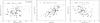 |
Fig. 1 Correlations between 6.7 GHz integrated flux density and beam-averaged H2 column density (left), between 6.7 GHz luminosity and mass (middle), and between 6.7 GHz luminosity and H2 volume density (right) of the associated 1.1 mm BGPS sources in the log-log plot. The dotted line in each panel represents the least-squares fit result to all data points. The correlation coefficient is also marked in each plot. Properties of the 6.7 GHz methanol masers are based on both this current survey and the literature (e.g., Caswell et al. 2010; Green et al. 2010; Szymczak et al. 2012), which are indicated by filled and open circles, respectively. |
P4636 G030.980+00.215. This new source has a single narrow feature near 110.9 km s-1 with a peak flux density of 1.0 Jy. IRAS 18443-0141, separated by ~110″, may be associated with it.
P4673 G031.077+00.459. This new source contains two main 6.7 GHz methanol features, one with a peak flux density of 2.1 Jy at ~25.7 km s-1 and another with a peak flux density of 1.4 Jy at ~26.5 km s-1. G031.0494+00.4698, an HII region separated by ~100″, may be associated with it (Urquhart et al. 2009).
P4701 G031.182-00.145. The spectrum of this new source contains several blended features spanning from 42.6 to 50.1 km s-1. An IRAS source 18461-0142 and an HII region, separated by ~80″ may be associated with it (Wood & Churchwell 1989; Becker et al. 1994).
P5050 G032.773-00.059. There are at least four features between 29.4 to 39.8 km s-1 with a peak flux density of 8.9 Jy at 38.5 km s-1. Toward G32.745-0.076 (IRAS 18487-0015), separated by ~118″, methanol emission was first found by Menten (1991) with a peak flux density of 46 Jy at ~38 km s-1. A similar value was reported by Caswell et al. (1995) and Szymczak et al. (2000, 2012). The aligned spectra suggest that our detection represents the sidelobe response from a nearby brighter source.
P5342 G034.264-00.210. There are three features in this new source, with a peak emission of 9.0 Jy at 54.6 km s-1. IRAS 18520+0101, separated by ~19″, may be associated with it. Apart from BGPS, no other research has been reported in this region.
P6323 G049.267-00.338 and P6346 G049.405-00.370. The two centers are separated by 513″, and shown on two aligned spectra in Fig. A.1. Prior knowledge about the known strong maser source G49.490-0.388 (offsets by 823″ and 313″, respectively) may lead to our observations. These sources are associated with the well-known complex W51. G049.267-00.338 is associated with an EGO (Cyganowski et al. 2008) as well as with a 95 GHz class I methanol maser (Chen et al. 2012).
P6414 G053.142+00.068 and P6433 G053.616+00.036. Two nearby known sources G53.142+0.071 (IRAS 19270+ 1750) and G53.618+0.036 (IRAS 19282+181) had peak flux densities of 1.9 Jy at 23.8 km s-1 and 6.3 Jy at 18.7 km s-1 when first detected by Szymczak et al. (2000). Recently, Szymczak et al. (2012) reported a flux density of 2.6 Jy at 23.8 km s-1 and 7.9 Jy at 18.9 km s-1. In our observation, the first source varied with a marginal detection of 0.6 Jy at 23.8 (fading by a factor of 0.25), while showing a peak flux density of 1.1 Jy at 24.7 km s-1. The second source shows a peak flux density of 6.0 Jy at 18.9 km s-1.
P6470 G056.962-00.234. This new source displays a narrow weak feature of 1.1 Jy. IRAS 19360+2101, separated by ~30″, may be associated with it.
P6479 G059.639-00.189. The spectrum is aligned with the velocity of the known maser G59.63-0.19 and separated by 23″ with a peak flux density of 3.3 Jy at 9.5 km s-1 (Szymczak et al. 2012).
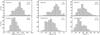 |
Fig. 2 Distributions of beam-averaged H2 column density (left), 1.1 mm integrated flux density (middle), and angular radius (right) of the BGPS sources for the two groups with and without 6.7 GHz class II methanol maser detections. Together with the standard deviation, the mean value is marked and indicated by a dotted line in each plot. |
Statistical parameters for sources with and without associated 6.7 GHz class II methanol masers for the entire sample.
4. Discussion
4.1. Characteristics of the 6.7 GHz class II methanol masers
For better comparison, the methods used by C2012 were adopted to estimate the properties summarized in Tables B.1, B.2, and Table 1, including luminosity, beam-averaged H2 column density, H2 number density and mass. A log-log plot of the beam-averaged H2 column density versus the integrated intensity of the 6.7 GHz methanol masers is shown in the left panel of Fig. 1. In addition, the log-log plots for the luminosity of the 6.7 GHz methanol masers as a function of the derived gas mass (middle panel) and H2 volume density (right panel) of the associated 1.1 mm BGPS source are also shown in Fig. 1. The results of a least-squares fit and the correlation coefficients are marked in each plot. The luminosity and flux of the 6.7 GHz methanol masers increase with the mass and column density of the associated dust clumps, as is evident in the left and middle panels of Fig. 1. The more luminous 6.7 GHz methanol masers are associated with less dense 1.1 dust clumps and can be seen in the right panel of Fig. 1, with a slope of −0.65 and a correlation coefficient of 0.35.
Similar trends have been revealed by Breen et al. (2010) with a sample of ~110 6.7 GHz methanol masers, which does not significantly overlap with our sample (about 10%). To explain these trends, Breen et al. (2010) proposed an evolutionary scenario, assuming that the methanol sources increase in luminosity as they evolve. This hypothesis has also been confirmed by their subsequent publication (Breen et al. 2011). Similarly, Wu et al. (2010) revealed that the lower luminosity 6.7 GHz methanol masers are associated with smaller ammonia line widths and therefore they correspond to the younger sources, which also agrees with the findings of Breen et al. (2010, 2011).
In comparison with the results of Breen et al. (2010), our data points show a relatively larger scatter. Nevertheless, our results might still support their hypothesis. As previously noted, properties of most methanol masers were extracted from the literature, referring to different telescopes and epochs. Therefore, the bias introduced by time variability and calibration uncertainties among different instruments may largely account for the scatter. Another possible explanation are false associations caused by the positional inaccuracies. In addition, for the new masers, the flux uncertainty introduced by relatively poor positional accuracy also contributes to the scatter. In the middle and right panels, bias introduced by inaccuracy of distances should be taken into account as well.
4.2. Statistical analysis of sources with and without associated 6.7 GHz class II methanol masers
Chen et al. (2011, 2012) revealed that there are no clear differences in the mid-IR colors between sources with and without associated class I methanol masers. However, the properties of masers (including water masers, class I and II methanol masers) heavily depend on the properties of the associated dust clumps (e.g., Breen et al. 2007, 2010; Breen & Ellingsen 2011; Chen et al. 2011, 2012). To further investigate whether there are any differences in properties of mid-IR and/or 1.1 mm dust clumps with and without associated class II methanol masers, a statistical analysis was performed following the methods of C2012 and Breen et al. (2007).
The dust clumps were split into two groups depending on either the presence or absence of class II methanol masers. Because we lack distance measurements for the latter group, the intrinsic physical parameters such as mass and source size in pc are not discussed in this section. Note that the beam-averaged H2 column density was directly derived from the S40″ (1.1 mm flux density within an aperture with a diameter of 40″), and therefore the S40″ was excluded from the following statistical analysis.
Figure 2 shows the distributions of the beam-averaged H2 column density (left panel), integrated flux density (middle panel), and angular radius (right panel), plotted as histograms for the two groups. Table 2 gives a summary of the basic statistical parameters, including the mean and median values and the standard deviations. We found that sources with associated 6.7 GHz class II methanol masers are more likely to have a higher column density, flux density, and radius than those without. The mean logarithmic value of column density of BGPS sources with class II methanol maser associations is 22.6 [cm-2], while it is 22.1 [cm-2] for those without. This result is expected because flux densities of BGPS sources will also fall off with distance (like methanol masers). The mean logarithmic value of the integrated flux density of BGPS sources with class II methanol maser associations is 0.6 [Jy], while it is 0.1 [Jy] for those without. A certain degree of discrepancy in column density and flux density does exist between the two groups with a difference of approximately two standard deviations. However, the difference in radius is less statistically significant, with a mean value of ~50′′ for both groups (a difference of less than one standard deviation). The mean values are marked in each corresponding panel of Fig. 2. The discovered trends are consistent with the results of C2012. Given the smaller overlap in the range of the beam-averaged column density for the two groups, as in C2012, we argue that the beam-averaged H2 column density might provide a better criterion for identifying possible BGPS sources with associated class II methanol masers.
In contrast, the color-color diagram of our sample in Fig. 3 shows that there is no significant difference in the nature of the associated GLIMPSE point sources between the two groups (indicated by solid and open circles), consistent with previous similar studies (e.g. Chen et al. 2011, 2012). Just as for the class I methanol masers in C2012, the detection rate of class II methanol masers is not closely related to the mid-IR property, which therefore cannot provide the most efficient criterion. On the other hand, one Effelsberg beam (~2′ at 6.7 GHz) would contain a number of GLIMPSE point sources, and in the present observations with this resolution we cannot distinguish which one is the true association. Our assumption that the GLIMPSE point source, which meets the mid-IR color criteria, is associated with the maser inevitably introduces false associations in some cases. Therefore we do not discuss the mid-IR property here in more detail.
4.2.1. Binomially generalized linear model
A binomially generalized linear model (GLM; McCullagh & Nelder 1989) was also fitted to the maser presence/absence using 1.1 mm BGPS properties, similar to the method used by Breen et al. (2007, 2010) and Breen & Ellingsen (2011). For a more detailed description of this analysis method see Breen et al. (2007). The probability of finding a maser in the ith clump, pi, can be predicted in terms of the clump properties x1ix2ix3i...xmi,
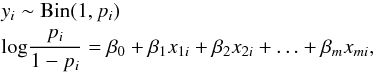 where yi is the maser
presence or absence in the ith clump and β0, β1,
β2...βm
are the regression coefficients.
where yi is the maser
presence or absence in the ith clump and β0, β1,
β2...βm
are the regression coefficients.
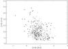 |
Fig. 3 Color–color diagram constructed from GLIMPSE point-source catalogs. Filled and open circles represent the sources with and without class II methanol maser detections, respectively. |
Analysis of deviance table for all possible single-term binomial models, including the AIC, associated likelihood ratio statistic and p-value.
First, a single-term binomial model was tested on each property and compared by
analyzing the deviance to the null model, which consists of only an intercept to
investigate whether individually they might give an indication for the probability of
finding an associated methanol maser. For each of the 332 dust clumps listed in Table
B.1 with available radius, the considered clump
properties were angular radius, integrated flux density (Sint) in Jy,
and beam-averaged H2 column density (NH2
1022
cm-3). Then,
the Akaike Information Criteria (AIC; Burnham & Anderson 2002) were used to select the most parsimonious model. P-values of less than
0.05 were considered to be statistically significant in the following analysis. All of
the possible single-term binomial models are summarized in Table 3. The results reveal that any one of these dust clump properties can
give an indication of the probability of methanol masers. The most simple model with the
greatest predictive power of maser presence involves only NH2. The estimated regression
relation can be expressed as 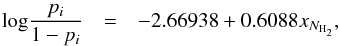 (1)where xNH2
is the beam-averaged H2 column density in 1022 cm-3. The regression summary of
this model is shown in Table 4. In general, the
results of the binomial model are consistent with the direct investigations outlined
above.
(1)where xNH2
is the beam-averaged H2 column density in 1022 cm-3. The regression summary of
this model is shown in Table 4. In general, the
results of the binomial model are consistent with the direct investigations outlined
above.
Estimated parameters for the binomial model using only NH2, including the regression coefficients and the standardized z-value and p-value for the test of the hypothesis that βi = 0.
4.3. 1.1 mm dust clumps with associated 6.7 GHz class II and/or 95 GHz class I methanol masers.
C2012 suggested that class I methanol masers with and without an associated 6.7 GHz class II methanol maser are different in the dust properties. However, limited by the small sample of 33 sources, they were unable to thoroughly investigate the star formation activities and physical properties of the class I and class II methanol masers.
As stated earlier, the sample of C2012 is covered by our sample, with only a few exceptions without valid data. In total, 194 (sources marked C in Table B.1) out of 214 sources in their sample had been studied in both the 6.7 GHz class II and 95 GHz class I methanol maser lines. This allows us to provide more meaningful constraints on the nature of BGPS sources with associated class I and class II methanol masers.
Similarly, the 194 overlapped clumps were split into four subgroups: sources with and without class II methanol masers and sources with and without class I methanol masers. The basic statistical parameters are summarized in Table 5. The trend drawn from the entire sample in the previous section is apparent in this smaller subsample as well. We also found that there is no significant statistical difference between sources with class I methanol masers and those with class II methanol masers, because the two groups share virtually the same mean values of beam-averaged H2 column density, 1.1 mm integrated flux density, and angular radius.
The 194 clumps with detectable methanol emissions were also split into the following three subgroups: (1) 36 sources in total with both class I and II methanol maser counterparts; (2) 17 sources in total with only class I methanol maser counterparts; and (3) 24 sources in total with only class II methanol maser counterparts. A comparison of the mass, beam-averaged H2 column density, and integrated flux density for the three subgroups is shown in Fig. 4. The derived statistical parameters are also summarized in Table 5. The first subgroup is found to show the highest mean and median values of mass, column density, and integrated flux (a difference of approximately two standard deviations). Comparing this sample with the smaller sample of C2012, we find that their results remain valid. We additionally find that the distributions of mass, column density, and flux density in the first subgroup cover the widest range. In general, there is no significant difference between the statistical results of the latter two categories.
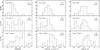 |
Fig. 4 Distributions of mass (left), beam-averaged H2 column density (middle), and 1.1 mm integrated flux density of the BGPS sources (right) for the three subgroups with only class I or class II detections and with both class I and class II detections. Together with the standard deviation, the mean value is marked and indicated by a dotted line in each plot. |
Statistical parameters for sources with and without associated methanol masers for the subsample overlapped with C2012.
Since class II methanol masers are thought to exclusively show traces of ongoing high-mass star formations (Walsh et al. 2001; Minier et al. 2003) and since class I methanol masers show traces of both high- and low-mass star formations (Kalenskii et al. 2006, 2010), it is reasonable to expect that sources with detectable class II methanol maser emissions have higher values of mass, column density and flux density than those with detectable class I methanol maser emissions. However, this alone cannot account for our findings in Fig. 4.
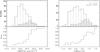 |
Fig. 5 Detection rates of class II methanol masers versus the BGPS beam-averaged H2 column density (left), and integrated flux density of the BGPS sources (right). For each BGPS property, the upper panel shows the histogram distributions of total sample sources (blank) and detected 6.7 GHz class II methanol maser sources (hatched), and the lower panel shows the corresponding detection rate of class II methanol maser in each statistical bin. |
It is important to keep in mind that properties of dust clumps can also change during the course of a maser’s evolution. For example, as a maser increases in flux density (and therefore luminosity), the dust clump becomes less dense and it continues to increase in mass, radius, and flux density (proposed by Breen et al. 2010, 2011, and also in this study). Once the evolutionary phase of a maser is taken into account, the situation will become more complicated. Ellingsen (2007) proposed a possible evolutionary sequence for the common maser species (class I and II methanol, water, and OH masers), which has recently been refined and quantified by Breen et al. (2010). They both proposed that the appearance and disappearance of class I methanol masers precede the class II methanol masers and do not overlap in time with OH masers (Ellingsen 2007; Breen et al. 2010). However, Voronkov et al. (2010) found that class I methanol masers do overlap in time with OH masers, which were thought to have a somewhat more evolved stage. To explain why sources with associated class I methanol masers have fainter red colors than those with associated class II methanol masers, Chen et al. (2011) suggested two epochs of class I methanol maser emission associated with high-mass star formation: an early epoch that significantly overlaps with the class II methanol maser phase, while the latter occurs after the class II methanol maser had faded out. Both studies suggested that the evolutionary phase of class I methanol masers needs to be revised.
4.4. Detection rates
Our single-dish survey, together with data from the literature, yields a detection rate of 26% of class II methanol masers of a sample of 391 sources with both 1.1 mm dust clump and GLIMPSE point source associations. For our 194 sources overlapped with C2012, the detection rates of class I and class II methanol masers are comparable, which are 28% and 31%, respectively. Generally, our detection rate is slightly lower than that of the other surveys with higher sensitivity, for example, a detection rate of ~35% for a sample of water masers with a sensitivity of 0.1–0.2 Jy (Xu et al. 2008).
To directly compare the relationships between the properties of the associated dust clumps and the detection rates of class II methanol masers, we plot the detection rates of class II methanol masers as a function of the BGPS beam-averaged H2 column density (left) and integrated flux density of the BGPS source (right) in Fig. 5. The detection rate is distinctly low in both low column density and low flux density ranges, while it increases dramatically with increasing column density and flux density.
The left panel of Fig. 6 shows the logarithm of the integrated flux density versus the beam-averaged H2 column density of BGPS sources with and without class II methanol maser associations (marked by red circles and green triangles, respectively) in our sample. The solid lines mark the boundary defined by C2012 in which most (90%) of their class I methanol maser detections are allocated. We find that 81% and 75% of detected class II methanol masers fall into their defined region for the overlapped subsample and the entire sample, respectively. Moreover, sources within their defined region correspond to a class II methanol maser detection rate of 52% for the smaller overlapped subsample, and 45% for the entire sample. To some extent, the new criteria for targeting 95 GHz class I methanol maser searches can also be applied to 6.7 GHz class II methanol maser searches, because the class II methanol maser detection rate is as high as 67% for sources with associated class I methanol maser in this current sample.
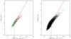 |
Fig. 6 Left panel: logarithm of the integrated flux density versus beam-averaged H2 column density of BGPS sources with and without class II methanol maser detections (marked by red circles and green triangles, respectively) in our current sample. The solid lines mark the boundary defined by Chen et al. (2012), while the dotted lines mark the slightly revised boundary. Right panel: same as left panel, but for all BGPS sources. |
Detection rates of class II methanol masers in different subsamples.
If the intercept of their defined region were slightly changed from −38 to −37.9, marked by the dotted line in Fig.
6, we would detect 83% of all expected class II
methanol masers of this study, and the sources that fall into the revised region would
correspond to a class II methanol maser detection rate of 43%. A comparison of the
detection rates of class II methanol masers in different subsamples is summarized in Table
6. Since our sample is much larger, we propose
that the revised boundary is as follows:  (2)which may be more appropriate for efficient
methanol maser searches, at least for class II methanol masers. In the right panel of Fig.
6 all BGPS sources are plotted. Approximately 1700
sources are located within the slightly revised boundary and ~700 of them are expected to be
associated with a class II methanol maser.
(2)which may be more appropriate for efficient
methanol maser searches, at least for class II methanol masers. In the right panel of Fig.
6 all BGPS sources are plotted. Approximately 1700
sources are located within the slightly revised boundary and ~700 of them are expected to be
associated with a class II methanol maser.
5. Summary
We reported results of a 6.7 GHz class II methanol maser survey using the Effelsberg 100 m radio telescope. A sample of 404 BGPS 1.1 mm dust clumps with GLIMPSE point-source associations was selected and 318 were observed. We detected 29 6.7 GHz methanol masers with flux densities in excess of the 3σ detection limit, 12 of which are new discoveries. Combining our results with the 74 detections directly from the literature, a total of 103 methanol masers are coincident with 1.1 mm dust clumps, which means an overall detection rate of 26%, similar to that of Chen et al. (2012).
The analysis of maser and 1.1 mm emissions revealed that the luminosity or flux of 6.7 GHz methanol masers increases with increasing mass or column density of the associated dust clump, whereas it decreases with increasing H2 number density of the associated dust clump. Our results support the evolutionary scenario presented in Breen et al. (2010).
We carried out a statistical analysis of the properties of the mid-IR and 1.1 mm dust clumps with or without 6.7 GHz class II methanol masers. We found that class II methanol masers are most likely associated with the brighter BGPS source. However, no significant difference between the two groups was found in properties of the mid-IR.
A comparison for the overlapped sample with C2012 of the 1.1 mm dust clump properties revealed that those associated with both class I and II methanol masers have the highest mean and median values of mass, column density, and integrated flux. There is no significant difference between statistical results of those with only class I methanol masers or those with only class II methanol masers. Because our sample is much larger, we revised the boundary defined by C2012 for efficiently selecting BGPS sources with an associated class II methanol maser, in which ~80% of the expected 6.7 GHz class II methanol masers will be detected with a detection rate in the range of 40–50%.
Acknowledgments
We are grateful to the staff of the Effelsberg 100 m radio telescope for their assistance in the observation. We would like to thank Alex Kraus for his help during the process of data calibration. We also thank the anonymous referee for a very helpful report and comments that helped to improve the paper. This work was supported by the National Natural Science Foundation of China (grants Nos. 11003046, 11133008, 11073054, 11233007, 10921063, 11073041 and 11273043), the Strategic Priority Research Program of the Chinese Academy of Sciences (grants Nos. XDA04060701 and XDB09000000), and the Key Laboratory for Radio Astronomy, CAS.
References
- Aguirre, J. E., Ginsburg, A. G., Dunham, M. K., et al. 2011, ApJS, 192, 4 [NASA ADS] [CrossRef] [MathSciNet] [Google Scholar]
- Becker, R. H., White, R. L., Helfand, D. J., & Zoonematkermani, S. 1994, ApJS, 91, 347 [NASA ADS] [CrossRef] [Google Scholar]
- Breen, S. L., & Ellingsen, S. P. 2011, MNRAS, 416, 178 [NASA ADS] [Google Scholar]
- Breen, S. L., Ellingsen, S. P., Johnston-Hollitt, M., et al. 2007, MNRAS, 377, 491 [NASA ADS] [CrossRef] [Google Scholar]
- Breen, S. L., Ellingsen, S. P., Caswell, J. L., & Lewis, B. E. 2010, MNRAS, 401, 2219 [NASA ADS] [CrossRef] [Google Scholar]
- Breen, S. L., Ellingsen, S. P., Caswell, J. L., et al. 2011, ApJ, 733, 80 [NASA ADS] [CrossRef] [Google Scholar]
- Burnham K. P., & Anderson D. R. 2002, Model Selection and Multimodel Inference, A Practical Information – Theoretic Approach, 2nd edn. (New York: Springer) [Google Scholar]
- Caswell, J. L. 2009, PASA, 26, 454 [NASA ADS] [CrossRef] [Google Scholar]
- Caswell, J. L., Vaile, R. A., Ellingsen, S. P., Whiteoak, J. B., & Norris, R. P. 1995, MNRAS, 272, 96 [NASA ADS] [CrossRef] [Google Scholar]
- Caswell, J. L., Fuller, G. A., Green, J. A., et al. 2010, MNRAS, 404, 1029 [NASA ADS] [CrossRef] [Google Scholar]
- Caswell, J. L., Fuller, G. A., Green, J. A., et al. 2011, MNRAS, 417, 1964 [NASA ADS] [CrossRef] [Google Scholar]
- Chen, X., Ellingsen, S. P., Shen, Z. Q., Titmarsh, A., & Gan, C. G. 2011, ApJS, 196, 9 [NASA ADS] [CrossRef] [Google Scholar]
- Chen, X., Ellingsen, S. P., He, J.-H., et al. 2012, ApJS, 200, 5 (C2012) [NASA ADS] [CrossRef] [Google Scholar]
- Chen, X., Gan, C. G., Ellingsen, S. P., et al. 2013, ApJS, 206, 22 [NASA ADS] [CrossRef] [Google Scholar]
- Cyganowski, C. J., Whitney, B. A., Holden, E., et al. 2008, AJ, 136, 2391 [NASA ADS] [CrossRef] [Google Scholar]
- Cyganowski, C. J., Brogan, C. L., Hunter, T. R., & Churchwell, E. 2009, ApJ, 702, 1615 [NASA ADS] [CrossRef] [Google Scholar]
- Dunham, M. K., Rosolowsky, E., Evans, N. J., II., Cyganowski, C., & Urquhart, J. S. 2011, ApJ, 741,110 [NASA ADS] [CrossRef] [Google Scholar]
- Ellingsen, S. P. 2006, ApJ, 638, 241 [NASA ADS] [CrossRef] [Google Scholar]
- Ellingsen, S. P. 2007, MNRAS, 377, 571 [NASA ADS] [CrossRef] [Google Scholar]
- Fontani, F., Cesaroni, R., & Furuya, R. S. 2010, A&A, 517, A56 [NASA ADS] [CrossRef] [EDP Sciences] [Google Scholar]
- Green, J. A., & McClure-Griffiths, N. M. 2011, MNRAS, 417, 2500 [NASA ADS] [CrossRef] [Google Scholar]
- Green, J. A., Caswell, J. L., Fuller, G. A., et al. 2009, MNRAS, 392, 783 [NASA ADS] [CrossRef] [Google Scholar]
- Green, J. A., Caswell, J. L., Fuller, G. A., et al. 2010, MNRAS, 409, 913 [NASA ADS] [CrossRef] [Google Scholar]
- Green, J. A., Caswell, J. L., Fuller, G. A., et al. 2012, MNRAS, 420, 3108 [NASA ADS] [CrossRef] [Google Scholar]
- Heyer, M., Krawczyk, C., Duval, J., & Jackson, J. M. 2009, ApJ, 699, 1092 [NASA ADS] [CrossRef] [Google Scholar]
- Kalenskii, S. V., Promyslov, V. G., Slysh, V. I., Bergman, P., & Winnberg, A. 2006, Astron. Rep., 50, 289 [NASA ADS] [CrossRef] [Google Scholar]
- Kalenskii, S. V., Johansson, L. E. B., Bergman, P., et al. 2010, MNRAS, 405, 613 [NASA ADS] [Google Scholar]
- Lee, H. T., Takami, M., Duan, H. Y., et al. 2012, ApJS, 200, 2 [NASA ADS] [CrossRef] [Google Scholar]
- Menten, K. M. 1991, ApJ, 380, 75 [Google Scholar]
- Minier, V., Ellingsen, S. P., Norris, R. P., & Booth, R. S. 2003, A&A, 403, 1095 [NASA ADS] [CrossRef] [EDP Sciences] [Google Scholar]
- Moscadelli, L., Xu, Y., & Chen, X. 2010, ApJ, 716, 1356 [NASA ADS] [CrossRef] [Google Scholar]
- Ott, M., Witzel, A., Quirrenbach, A., et al. 1984, A&A, 284, 331 [Google Scholar]
- Pandian, J. D., Goldsmith, P. F., & Deshpande, A. A. 2007, ApJ, 656, 255 [NASA ADS] [CrossRef] [Google Scholar]
- Pandian, J. D., Momjian, E., Xu, Y., Menten, K. M., & Goldsmith, P. F. 2011, ApJ, 730, 55 [NASA ADS] [CrossRef] [Google Scholar]
- Pestalozzi, M. R., Minier, V., & Booth, R. S. 2005, A&A, 432, 737 [NASA ADS] [CrossRef] [EDP Sciences] [Google Scholar]
- Reid, M. J., Menten, K. M., Zheng, X. W., et al. 2009, ApJ, 700, 137 [NASA ADS] [CrossRef] [Google Scholar]
- Rosolowsky, E., Dunham, M. K., Ginsburg, A., et al. 2010, ApJS, 188, 123 [NASA ADS] [CrossRef] [Google Scholar]
- Schlingman, W. M., Shirley, Y. L., Schenk, D. E., et al. 2011, ApJS, 195, 14 [NASA ADS] [CrossRef] [Google Scholar]
- Sridharan, T. K., Beuther, H., Schilke, P., Menten, K. M., & Wyrowski, F. 2002, ApJ, 566, 931 [NASA ADS] [CrossRef] [Google Scholar]
- Szymczak, M., Hrynek, G., & Kus, A. J. 2000, A&AS, 143, 269 [NASA ADS] [CrossRef] [EDP Sciences] [Google Scholar]
- Szymczak, M., Wolak, P., Bartkiewicz, A., & Borkowski, K. M. 2012, Astron. Nachr., 333, 634 [NASA ADS] [CrossRef] [Google Scholar]
- Urquhart, J. S., Hoare, M. G., Purcell, C. R., et al. 2009, A&A, 501, 539 [NASA ADS] [CrossRef] [EDP Sciences] [Google Scholar]
- Voronkov, M. A., Caswell, J. L., Ellingsen, S. P., & Sobolev, A. M. 2010, MNRAS, 405, 2471 [NASA ADS] [Google Scholar]
- Walsh, A. J., Bertoldi, F., Burton, M. G., & Nikola, T. 2001, MNRAS, 326, 36 [NASA ADS] [CrossRef] [Google Scholar]
- Wood, D. O. S., & Churchwell, E. 1989, ApJS, 69, 831 [NASA ADS] [CrossRef] [Google Scholar]
- Wu, Y. W., Xu, Y., Pandian, J. D., et al. 2010, ApJ, 720, 392 [NASA ADS] [CrossRef] [Google Scholar]
- Xu, Y., Li, J. J., Hachisuka, K., et al. 2008, A&A, 485, 729 [NASA ADS] [CrossRef] [EDP Sciences] [Google Scholar]
- Xu, Y., Voronkov, M. A., Pandian, J. D., et al. 2009, A&A, 507, 1117 [NASA ADS] [CrossRef] [EDP Sciences] [Google Scholar]
Appendix A:
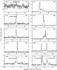 |
Fig. A.1 Spectra of the 6.7 GHz methanol masers, in units of Jy. The spectral extent is marked in the highly variable source G06.189-0.358 and in seven sources that may have suffered from confusion due to strong adjacent sources. The rms for each spectrum and the PID number of each associated BGPS source are marked in the upper left and upper right corners, respectively. The spectra have a resolution of 0.11 km s-1. |
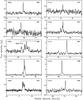 |
Fig. A.1 continued. |
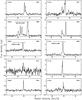 |
Fig. A.1 continued. |
Appendix B:
Parameters of the target BGPS and GLIMPSE sources.
Related parameters of the class II methanol masers from the literature.
All Tables
Related parameters of the class II methanol masers observed with the Effelsberg 100 m radio telescope.
Statistical parameters for sources with and without associated 6.7 GHz class II methanol masers for the entire sample.
Analysis of deviance table for all possible single-term binomial models, including the AIC, associated likelihood ratio statistic and p-value.
Estimated parameters for the binomial model using only NH2, including the regression coefficients and the standardized z-value and p-value for the test of the hypothesis that βi = 0.
Statistical parameters for sources with and without associated methanol masers for the subsample overlapped with C2012.
All Figures
|
Fig. 1 Correlations between 6.7 GHz integrated flux density and beam-averaged H2 column density (left), between 6.7 GHz luminosity and mass (middle), and between 6.7 GHz luminosity and H2 volume density (right) of the associated 1.1 mm BGPS sources in the log-log plot. The dotted line in each panel represents the least-squares fit result to all data points. The correlation coefficient is also marked in each plot. Properties of the 6.7 GHz methanol masers are based on both this current survey and the literature (e.g., Caswell et al. 2010; Green et al. 2010; Szymczak et al. 2012), which are indicated by filled and open circles, respectively. |
| In the text | |
|
Fig. 2 Distributions of beam-averaged H2 column density (left), 1.1 mm integrated flux density (middle), and angular radius (right) of the BGPS sources for the two groups with and without 6.7 GHz class II methanol maser detections. Together with the standard deviation, the mean value is marked and indicated by a dotted line in each plot. |
| In the text | |
|
Fig. 3 Color–color diagram constructed from GLIMPSE point-source catalogs. Filled and open circles represent the sources with and without class II methanol maser detections, respectively. |
| In the text | |
|
Fig. 4 Distributions of mass (left), beam-averaged H2 column density (middle), and 1.1 mm integrated flux density of the BGPS sources (right) for the three subgroups with only class I or class II detections and with both class I and class II detections. Together with the standard deviation, the mean value is marked and indicated by a dotted line in each plot. |
| In the text | |
|
Fig. 5 Detection rates of class II methanol masers versus the BGPS beam-averaged H2 column density (left), and integrated flux density of the BGPS sources (right). For each BGPS property, the upper panel shows the histogram distributions of total sample sources (blank) and detected 6.7 GHz class II methanol maser sources (hatched), and the lower panel shows the corresponding detection rate of class II methanol maser in each statistical bin. |
| In the text | |
|
Fig. 6 Left panel: logarithm of the integrated flux density versus beam-averaged H2 column density of BGPS sources with and without class II methanol maser detections (marked by red circles and green triangles, respectively) in our current sample. The solid lines mark the boundary defined by Chen et al. (2012), while the dotted lines mark the slightly revised boundary. Right panel: same as left panel, but for all BGPS sources. |
| In the text | |
|
Fig. A.1 Spectra of the 6.7 GHz methanol masers, in units of Jy. The spectral extent is marked in the highly variable source G06.189-0.358 and in seven sources that may have suffered from confusion due to strong adjacent sources. The rms for each spectrum and the PID number of each associated BGPS source are marked in the upper left and upper right corners, respectively. The spectra have a resolution of 0.11 km s-1. |
| In the text | |
|
Fig. A.1 continued. |
| In the text | |
|
Fig. A.1 continued. |
| In the text | |
Current usage metrics show cumulative count of Article Views (full-text article views including HTML views, PDF and ePub downloads, according to the available data) and Abstracts Views on Vision4Press platform.
Data correspond to usage on the plateform after 2015. The current usage metrics is available 48-96 hours after online publication and is updated daily on week days.
Initial download of the metrics may take a while.