| Issue |
A&A
Volume 563, March 2014
|
|
|---|---|---|
| Article Number | L1 | |
| Number of page(s) | 6 | |
| Section | Letters | |
| DOI | https://doi.org/10.1051/0004-6361/201323028 | |
| Published online | 25 February 2014 | |
First results from the CALYPSO IRAM-PdBI survey
I. Kinematics of the inner envelope of NGC 1333-IRAS2A⋆,⋆⋆,⋆⋆⋆
1 UJF-Grenoble 1/CNRS-INSU, Institut de Planétologie et d’Astrophysique de Grenoble, UMR 5274, 38041 Grenoble, France
e-mail: This email address is being protected from spambots. You need JavaScript enabled to view it.
2 Max-Planck-Institut für Radioastronomie, Auf dem Hügel 69, 53121 Bonn, Germany
3 Harvard-Smithsonian Center for Astrophysics, 60 Garden street, Cambridge MA 02138, USA
4 IRAM, 300 rue de la piscine, 38406 Saint Martin d’Hères, France
5 Laboratoire AIM-Paris-Saclay, CEA/DSM/Irfu – CNRS – Université Paris Diderot, CE-Saclay, 91191 Gif-sur-Yvette, France
6 LERMA, Observatoire de Paris, CNRS, ENS, UPMC, UCP, 61 Av de l’Observatoire, 75014 Paris, France
7 INAF – Osservatorio Astrofisico di Arcetri, Largo E. Fermi 5, 50125 Firenze, Italy
8 Université de Bordeaux, LAB, UMR 5804, 33270 Floirac, France
9 CNRS, LAB, UMR 5804, 33270 Floirac, France
Received: 11 November 2013
Accepted: 22 January 2014
Abstract
The structure and kinematics of Class 0 protostars on scales of a few hundred AU is poorly known. Recent observations have revealed the presence of Keplerian disks with a diameter of 150–180 AU in L1527-IRS and VLA1623A, but it is not clear if such disks are common in Class 0 protostars. Here we present high-angular-resolution observations of two methanol lines in NGC1333-IRAS2A. We argue that these lines probe the inner envelope, and we use them to study the kinematics of this region. Our observations suggest the presence of a marginal velocity gradient normal to the direction of the outflow. However, the position velocity diagrams along the gradient direction appear inconsistent with a Keplerian disk. Instead, we suggest that the emission originates from the infalling and perhaps slowly rotating envelope, around a central protostar of 0.1−0.2 M⊙. If a disk is present, it is smaller than the disk of L1527-IRS, perhaps suggesting that NGC 1333-IRAS2A is younger.
Key words: ISM: individual objects: NGC 1333-IRAS2A / ISM: kinematics and dynamics / ISM: molecules / stars: formation
Based on observations carried out with the IRAM Plateau de Bure interferometer. IRAM is supported by INSU/CNRS (France), MPG (Germany), and IGN (Spain).
Table 1 and Appendix A are available in electronic form at http://www.aanda.org
Reduced PdBI data are available at the CDS via anonymous ftp to cdsarc.u-strasbg.fr (130.79.128.5) or via http://cdsarc.u-strasbg.fr/viz-bin/qcat?J/A+A/563/L1
© ESO, 2014
1. Introduction
Understanding the first steps of the formation of protostars and protoplanetary disks is a major unsolved problem of modern astrophysics. Observationally, the key to constraining protostar formation models lies in high-resolution studies of the youngest protostars. Because their lifetime is only t ~ 105 yr and most of their mass is still in the form of a dense envelope (M∗ ≪ Menv), Class 0 protostars are likely to retain detailed information on the initial conditions and detailed physics of the collapse phase (André et al. 2000). However, the physics of Class 0 protostars is still surprisingly poorly understood, due to the paucity of the sub-arcsecond (sub)mm observations required to probe their innermost (100 AU) regions. Several basic questions thus remain open, such as the mere existence of accretion disks during the Class 0 phase, or the structure of the velocity field in Class 0 envelopes (e.g., relative importance of inflow, rotation, and outflow). On the large scales, some of the Class 0 sources show evidence of flattened structures, extending roughly perpendicular to the outflow over ≥10 000 AU (Belloche et al. 2002; Looney et al. 2007; Tobin et al. 2010). However, line observations indicate that these structures are slowly rotating infalling envelopes rather than centrifugally supported disks (Belloche et al. 2002; Chiang et al. 2010). On smaller scales (several hundred AU), little is known on the envelope/disk structure and kinematics. Only two Class 0 protostars, L1527-IRS and VLA1623A, show an evidence of a compact (150 AU to 180 AU in diameter) Keplerian disk (Tobin et al. 2012; Murillo et al. 2013). Studying these regions requires observations of specific (optically thin) tracers of the inner region to avoid contamination by the outflow and the extended envelope. Methanol lines are good specific probes of these regions, as we discuss below.
In this letter, we present observations of two methanol lines in the NGC1333-IRAS2A Class 0 protostar (hereafter IRAS2A) located in the Perseus molecular complex at 235 pc (Hirota et al. 2008). These observations are part of the CALYPSO (Continuum And Line in Young Proto-Stellar Objects) survey1, an IRAM Plateau de Bure Interferometer (hereafter PdBI) large program that aims at studying a large sample of Class 0 protostars at sub-arcsecond resolution. We use these lines to probe the kinematics of the protostellar envelope on ~200 AU scales, and to determine if a disk is present. Two companion Letters present the complex organic molecule (COM) emission (Maury et al. 2014) and the jet properties (Codella et al. 2014).
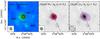 |
Fig. 1 Continuum and line emissions observed towards IRAS2A with the PdBI. The left panel shows the 1 mm continuum emission. Contour spacing is 10 mJy beam-1 (6.6σ). The other panels show the velocity integrated intensities of the 1 mm and 3 mm methanol lines (blue and red contours) together with the continuum (grayscale image). The blue and red contours correspond to velocities <6.5 km s-1 and >6.5 km s-1, respectively. In the center panel, the blue and red contours are almost coincident. The contour spacings are 100 mJy beam-1 km s-1 (3.2σ) and 30 mJy beam-1 km s-1 (2.1σ) for the 1 mm and 3 mm lines, respectively. In each panel the dashed ellipse indicates the size and orientation of the synthesized beam. The dashed line shows the orientation of the outflow (which has a PA of 25°; Codella et al. 2014). |
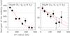 |
Fig. 2 Real part of the visibility of the 1 mm (left panel) and 3 mm (right panel) methanol lines as a function of the UV radius (black points with error bars). The visibilities have been averaged over the line profile, and then averaged circularly. The solid red line in each panel shows the result of a Gaussian source fit, while the dotted red line shows the result of a point source fit. The dashed line in the right panel shows the result of a Gaussian source fit with a FWHM size fixed to that of the 1 mm line (0.44″). The dotted black line in each panel indicates the zero level. |
2. Observations
Observations of IRAS2A were carried out with the PdBI between November 2010 and February 2011 using the A and C configurations of the array. The CH3OH (51−42 νt = 0 E1) line at 216.945 600 GHz (1 mm) was observed using the narrow-band backend, providing a bandwidth of 512 channels of 39 kHz (0.05 km s-1) each. The CH3OH (10−21 νt = 1 E1) line at 93.196 670 GHz (3 mm) was also observed using the narrow-band backend, but with 256 channels of 312 kHz (1.0 km s-1) each. Calibration was done using CLIC, which is part of the GILDAS software suite2. For the 1 mm observations, the phase RMS was <80°, with precipitable water vapor (PWV) between 0.5 mm and 2 mm, and system temperatures (Tsys) between 100 K and 250 K. For the 3 mm observations, the phase RMS was <40°, with PWV of 2–3 mm and Tsys of 70–80 K. The continuum emission was removed from the visibility tables to produce continuum-free line tables. The visibilities of the 1 mm methanol line were resampled at a spectral resolution of 0.5 km s-1 to improve the signal-to-noise ratio. Spectral datacubes were produced from the visibility tables using a natural weighting, and deconvolved using the standard CLEAN algorithm in the MAPPING program. The synthesized beam is 0.79″ × 0.76″ (PA 70°) and 1.71″ × 1.31″ (PA 54°) for the 1 mm and 3 mm lines, respectively. The RMS noise per channel in the final datacubes is 21 mJy/beam and 5 mJy/beam for the 1 mm and 3 mm lines, respectively.
3. Results and analysis
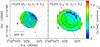 |
Fig. 3 First-order moment maps of the 1 mm (left panel) and 3 mm (right panel) methanol lines. In each panel the solid contours show the velocity integrated line intensity. The contour spacings are 200 mJy beam-1 km s-1 and 20 mJy beam-1 km s-1 for the 1 mm and 3 mm methanol lines, respectively. The dashed line shows the orientation of the outflow, while the dashed arrow indicates the orientation of the velocity gradient as determined from the first-order moment fit (see Sect. 3). The line and arrow intersect at the position of MM1. |
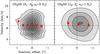 |
Fig. 4 Position-velocity diagrams for the 1 mm (left panel) and 3 mm (right panel) methanol lines. The contour spacing is 50 mJy beam-1 (2.4σ) and 10 mJy beam-1 (2σ) for the 1 mm and 3 mm methanol lines, respectively. The red points with error bars show the first order moment measured at each position offset. The horizontal dashed line shows the source vLSR (6.5 km s-1). The vertical dashed lines indicate the center of the cut. |
Figure 1 shows the 1 mm continuum emission together with velocity integrated intensity maps of the 1 mm and 3 mm methanol lines. Continuum emission is detected in three sources, which are labeled MM1, MM2, and MM3 in Codella et al. (2014). We detect 1 mm and 3 mm methanol line emission towards the brightest continuum peak (MM1) with a signal-to-noise ratio at the line peaks of 21 and 8 for the 1 mm and 3 mm methanol lines, respectively. Emission from these lines is compact. In addition, no clear difference between the blue-shifted and red-shifted emission (at velocities <6.5 km s-1 and >6.5 km s-1, respectively3) is seen.
To determine the size of the line emission, we fitted the visibilities assuming that the emission follows a Gaussian distribution. We averaged the visibilities over the entire velocity range of the line, and we performed a fit of the velocity averaged visibilities in the UV plane. Figure 2 shows the result of the fit, together with the real part of the visibilities (averaged as a function of the UV radius for clarity). The fit parameters are given in Table 1. As seen in Fig. 2, the 1 mm methanol line emission is spatially resolved, and it is reasonably well fitted by a Gaussian source with a FWHM size of 0.44 ± 0.03″. On the other hand, the 3 mm methanol line is only marginally resolved; the emission is best fitted by a Gaussian of 0.59 ± 0.11″ FWHM, but its size is also consistent (at a 2σ level) with that of the 1 mm line. This is also apparent in the right panel of Fig. 2, which shows the expected real part of the visibility for the 3 mm line, assuming a Gaussian source of 0.44″. The position of the 1 mm methanol line peak is, within the uncertainties, consistent with the position of the MM1 continuum source. Although the position of the 3 mm methanol line appears slightly offset, it is also consistent (at a 5σ level) with the position of MM1. Table 1 also gives the linewidths at the position of the 1 mm line emission peak. Both the 1 mm and 3 mm lines have Gaussian shapes, with a FWHM of 3.3 and 4.1 km s-1, respectively.
Figure 3 shows the first-order moment (mean velocity) maps for both lines. From visual inspection of the moment maps, no clear velocity gradient is apparent. We have therefore attempted to fit the first order moment maps with a linear function of the RA and Dec offsets. This linear gradient is expected if the emitting region is rotating as a solid body (Goodman et al. 1993). Although solid body rotation is not realistic, it provides a first indication of whether or not rotation is present. Because the maps shown in Fig. 3 are oversampled, we have fitted the first-order moment measured every half synthesized beam (Nyquist sampling). These pixels were weighted by 1/σ2, where σ is the 1σ noise on the first-order moment, computed from the noise per channel in the data cubes (see Belloche 2013, Eq. (2.3)). Results of the fit are given in Table 1. For the 1 mm line, we find a gradient with a PA α = 107 ± 27° and an amplitude G = 0.23 ± 0.11 km s-1 /″ (202 ± 97 km s-1 /pc at 235 pc). For the 3 mm, we find α = 131 ± 36° and G = 0.47 ± 0.29 km s-1 /″ (413 ± 255 km s-1 /pc). Although the gradient detection is only marginal (2.1σ and 1.6σ for the values of G at 1 mm and 3 mm, respectively), the amplitude and orientation obtained for each line are consistent. The gradient orientations are indicated by arrows in Fig. 3. Interestingly, they are roughly perpendicular to the outflow orientation, as one would expect for rotation of the protostellar envelope or disk.
Figure 4 shows the position-velocity (hereafter PV) diagrams for both lines. The cuts were done along an axis with PA of 107°, and centered on the peak of the 1 mm line. Figure 4 also shows the first-order moment measured along the cut. No clear signature of rotation is apparent in the P.V. diagram. Both diagrams are almost symmetric with respect to the cut center position. However, the first-order moment measured along the cut increases from negative to positive offsets. This is consistent with the presence of a gradient along this axis. This increase in the first-order moment along the cut is also marginal (see the error bars in Fig. 4), but the same trend is seen for both lines.
4. Discussion and conclusions
Our observations reveal compact methanol emission (0.4″ FWHM, i.e., ~90 AU in diameter) centered on the position of the MM1 continuum source. The observed emission has several possible origins. First, methanol emission can arise from shocks, as a result of ice sputtering; indeed, methanol emission is observed towards the end points of the large scale east-west outflow of IRAS2A (Bachiller et al. 1998). It is therefore possible that the emission observed here is caused by shocks on smaller scales. However, the line Gaussian shapes and small linewidths, together with the striking contrast between the methanol and the SO and SiO emission (which are associated with the shocked gas; see Codella et al. 2014), do not favor this hypothesis.
Second, the emission may arise from the inner region of the envelope where the temperature is greater than ~100 K (the so-called hot corino). Maret et al. (2005) did a single-dish survey of the methanol emission from a sample of six Class 0 protostars, and found abundance jumps (by about 2 orders of magnitude) in the inner envelopes of four of them (including IRAS2A). They interpreted these abundance jumps as due to the thermal evaporation of grain mantles in the hot corino. Several COMs, such as acetonitrile, methyl formate, or dimethyl ether, have also been detected in IRAS2A with single-dish (Bottinelli et al. 2007) and interferometric (Maury et al. 2014) observations. The similar COM (Maury et al. 2014) and methanol emission sizes (this study) strongly suggest a common origin. Compact water (H O) emission has also been detected in IRAS2A with the PdBI (Persson et al. 2012). The size of the HO emission (0.8′′) is twice as large as the methanol emission. However, the HO maps show some emission associated with the outflow. This contamination by the outflow may explain the larger extension of the HO emission with respect to the methanol and the COM emission. Dust continuum observations and modeling indicate that the radius at which the dust temperature exceeds 100 K in IRAS2A is about 50 AU (Jørgensen et al. 2002)4. This radius is in good agreement with the size of the methanol emission, and therefore favors the hot corino scenario.
A third scenario is that the emission originates from the surface of a disk. From SMA observations of the dust continuum, Jørgensen et al. (2005) suggested that IRAS2A harbors a circumstellar disk of 200–300 AU in diameter, with a mass between 0.01 M⊙ and 0.1 M⊙. They suggested that the disk could be the major reservoir of the COMs and other molecules observed in that source. Brinch et al. (2009) modeled the HCN and H13CN (4–3) emission observed with the SMA towards IRAS2A at 1″ resolution, and found that the velocity field was dominated by infall, with little rotation. A flattened disk-like structure dominated by inward motions is also favored by Persson et al. (2012) to explain the HO emission observed in IRAS2A. Our methanol observations suggest the presence of a marginal velocity gradient oriented roughly in a direction perpendicular to the north-south outflow. The orientation of the gradient is similar to that of a second east-west outflow detected in this source. However, this second outflow is probably driven by the MM2 source and its axis does not pass through the position of MM1 (Codella et al. 2014), while the methanol emission is clearly associated with MM1. Therefore, the gradient is most likely caused by rotation of the inner envelope or a disk about the outflow axis.
Regardless of the origin of the emission (i.e., hot corino or disk), if the material traced by the methanol lines is bound to the protostellar system (as opposed to unbound outflow material for example), the line width can be used to estimate the dynamical mass of the system, Mdyn ~ (1 − 2) r v2/G, where v is the velocity observed at a radii r, and G is the gravitational constant. This expression holds if the line broadening is due to infall motions, or Keplerian rotation about an axis close to the plane-of-the-sky (see, e.g., Terebey et al. 1992). If we assume that the velocity at r = 45 AU is 1.65 km s-1 (i.e., the 1 mm line HWHM), we obtain Mdyn ≃ 0.1 − 0.2 M⊙(to be compared to a total envelope mass Menv = 1.7M⊙; Jørgensen et al. 2002). Strictly speaking, Mdyn is the mass contained within a radius of 45 AU, so that M∗ ≲ 0.1 − 0.2 M⊙. This estimate is in reasonable agreement with the value of 0.25 M⊙ obtained by Brinch et al. (2009).
The 1 mm line P.V. diagram can be used to test the disk scenario. We have computed synthetic P.V. diagrams for a Keplerian disk with various values of M∗ (see Appendix A for details).
We find that the observed P.V. diagram is inconsistent with a Keplerian disk, regardless of the mass of the central object. In particular, a Keplerian disk with M∗ = 0.1 M⊙ would produce two peaks in the P.V. diagram, which are not observed. On the other hand, a Keplerian disk M∗ = 0.01 M⊙ would have a single peak P.V. diagram, but the predicted linewidth would be 2–3 times smaller than observed, even for a very turbulent disk.
To summarize, we favor a scenario in which the methanol emission observed in IRAS2A originates in the inner envelope of the protostar, which is infalling and perhaps slowly rotating. If a disk is present and is emitting in methanol, it is spatially unresolved so its radius is smaller than 45 AU (0.4′′), i.e. smaller than the disk of L1527-IRS. Since the mass of the central object in L1527-IRS (0.2 M⊙; Tobin et al. 2012) is comparable to that of IRAS2A, this may suggest that IRAS2A is younger. Higher angular resolution observations are needed to confirm the presence of rotation in the inner parts of IRAS2A and to measure the rotation profile precisely. In addition, observations of other Class 0 protostars are needed to obtain more statistics on the presence of rotationaly supported disks in this phase, and to establish when disks appear during the evolution of protostars.
Online material
Line spectroscopic parameters, results of the visibility fits, and results of the first-order moment fits.
Appendix A: Synthetic position velocity diagrams for a Keplerian disk
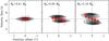 |
Fig. A.1 Synthetic position-velocity diagrams for the 1 mm methanol line (gray contours). The contour levels and axis ranges are the same as in Fig. 4. The red points with error bars show the line centroid along the cut. The diagrams have been computed assuming that the emission originates in a Keplerian disk with different masses of the central protostar (see text). |
To test the Keplerian disk scenario, we have computed synthetic P.V. diagrams for the 1 mm methanol line. We have assumed that the emission follows a Gaussian distribution, with a FWHM of 0.44′′ (as determined from the visibility fit). The line-of-sight velocity is assumed to be given by (see, e.g., Guilloteau et al. 2012)  (A.1)where r and θ are the cylindrical coordinates in the disk plane, i is the inclination of the disk rotation axis with respect to the line of sight (i.e., i = 90° for an edge-on disk), vLSR is the source
velocity in the local standard of rest, and  is the Keplerian velocity
  (A.2)with G the gravitational constant and M∗ the mass of the central protostar. The line is assumed to have a Gaussian shape, with a local linewidth
  (
( ) equal to
  , in agreement with the value determined in DM Tau by Guilloteau et al. (2012). Although this value is uncertain, it cannot exceed because a disk with a larger would be unstable. We assume that the disk is rotating about an axis with i = 60°. This is consistent with the disk rotating about the outflow axis, which has i ≥ 45° (Codella et al. 2014). Finally, we assume a vLSR of 6.5 km s-1, a source distance of 235 pc, and M∗ is left as a free parameter. The disk is not truncated in radius; we merely assume that its line emission decreases as a Gaussian, as mentioned above. We compute a synthetic data cube with a pixel size of 0.1″, and a channel width of 0.5 km s-1. The intensity of the emission as a function of channel is computed assuming that the line-of-sight velocity varies as a function of r and θ following Eq. (A.1). This data cube is then convolved with the synthesized beam, assumed to be a Gaussian with a FWHM of 0.8′′. The convolved data cube is then scaled so that the peak intensity matches the observations (453 mJy/beam). Finally, Gaussian noise is added in each channel so that the signal-to-noise ratio also corresponds to the observations (~21).
Figure A.1 shows the synthetic position velocity diagrams we obtain for different values of M∗. We find that our observations are inconsistent with a Keplerian disk, regardless of the mass of the central object. For M∗ = 0.05 M⊙ and 0.1 M⊙, the synthetic P.V. diagrams have two peaks, while the observed P.V. diagram has one peak (see Fig. 4). For M∗ = 0.01 M⊙, the synthetic P.V. diagram is single peaked, and the predicted first-order moment along the cut is constant, within the error bars. However, the predicted linewidth is much smaller than observed (compare the size of the P.V. contours along the vertical axis in Figs. 4 and A.1). A broader linewidth would require a larger value of . However, we find that even for a very turbulent disk with  , the predicted linewidth is 2–3 times smaller than observed. We conclude that the observed methanol emission can not arise from a Keplerian disk, and must originate in the infalling and perhaps slowly rotating inner envelope. A more detailed modeling of the methanol line emission is needed to determine the precise velocity field of the inner region of the protostar envelope.
In the present study, we adopt a vLSR of 6.5 km s-1, as determined from a fit of the first-order moment map of the 1 mm methanol line (see further).
A more recent analysis suggests a larger value (90 AU; Kristensen et al. 2012).
Acknowledgments
The research leading to these results has received funding from the European Community’s Seventh Framework Programme (/FP7/2007-2013/) under grant agreements No. 229517 (ESO COFUND) and No. 291294 (ORISTARS), and from the French Agence Nationale de la Recherche (ANR), under reference ANR-12-JS05-0005.
References
- André, P., Ward-Thompson, D., & Barsony, M. 2000, in Protostars and Planets IV (Tucson: University of Arizona Press), 59 [Google Scholar]
- Bachiller, R., Codella, C., Colomer, F., Liechti, S., & Walmsley, C. M. 1998, A&A, 335, 266 [Google Scholar]
- Belloche, A. 2013, in EAS Publ. Ser., 62, 25 [Google Scholar]
- Belloche, A., André, P., Despois, D., & Blinder, S. 2002, A&A, 393, 927 [Google Scholar]
- Bottinelli, S., Ceccarelli, C., Williams, J. P., & Lefloch, B. 2007, A&A, 463, 601 [NASA ADS] [CrossRef] [EDP Sciences] [Google Scholar]
- Brinch, C., Jørgensen, J. K., & Hogerheijde, M. R. 2009, A&A, 502, 199 [NASA ADS] [CrossRef] [EDP Sciences] [Google Scholar]
- Chiang, H., Looney, L. W., Tobin, J. J., & Hartmann, L. 2010, ApJ, 709, 470 [Google Scholar]
- Codella, C., Maury, A. J., Gueth, F., et al. 2014, A&A, 563, L3 [NASA ADS] [CrossRef] [EDP Sciences] [Google Scholar]
- Goodman, A. A., Benson, P. J., Fuller, G. A., & Myers, P. C. 1993, ApJ, 406, 528 [NASA ADS] [CrossRef] [Google Scholar]
- Guilloteau, S., Dutrey, A., Wakelam, V., et al. 2012, A&A, 548, A70 [NASA ADS] [CrossRef] [EDP Sciences] [Google Scholar]
- Hirota, T., Bushimata, T., Choi, Y. K., et al. 2008, PASJ, 60, 37 [NASA ADS] [CrossRef] [Google Scholar]
- Jørgensen, J. K., Schöier, F. L., & van Dishoeck, E. F. 2002, A&A, 389, 908 [NASA ADS] [CrossRef] [EDP Sciences] [Google Scholar]
- Jørgensen, J. K., Bourke, T. L., Myers, P. C., et al. 2005, ApJ, 632, 973 [NASA ADS] [CrossRef] [Google Scholar]
- Kristensen, L. E., van Dishoeck, E. F., Bergin, E. A., et al. 2012, A&A, 542, A8 [NASA ADS] [CrossRef] [EDP Sciences] [Google Scholar]
- Looney, L. W., Tobin, J. J., & Kwon, W. 2007, ApJ, 670, L131 [NASA ADS] [CrossRef] [Google Scholar]
- Maret, S., Ceccarelli, C., Tielens, A. G. G. M., et al. 2005, A&A, 442, 527 [NASA ADS] [CrossRef] [EDP Sciences] [Google Scholar]
- Maury, A. J., Belloche, A., André, P., et al. 2014, A&A, 563, L2 [NASA ADS] [CrossRef] [EDP Sciences] [Google Scholar]
- Müller, H. S. P., Thorwirth, S., Roth, D. A., & Winnewisser, G. 2001, A&A, 370, L49 [NASA ADS] [CrossRef] [EDP Sciences] [Google Scholar]
- Murillo, N. M., Lai, S.-P., Bruderer, S., Harsono, D., & van Dishoeck, E. F. 2013, A&A, 560, A103 [NASA ADS] [CrossRef] [EDP Sciences] [Google Scholar]
- Persson, M. V., Jørgensen, J. K., & van Dishoeck, E. F. 2012, A&A, 541, A39 [NASA ADS] [CrossRef] [EDP Sciences] [Google Scholar]
- Terebey, S., Vogel, S. N., & Myers, P. C. 1992, ApJ, 390, 181 [NASA ADS] [CrossRef] [Google Scholar]
- Tobin, J. J., Hartmann, L., Looney, L. W., & Chiang, H.-F. 2010, ApJ, 712, 1010 [NASA ADS] [CrossRef] [Google Scholar]
- Tobin, J. J., Hartmann, L., Chiang, H.-F., et al. 2012, Nature, 492, 83 [NASA ADS] [CrossRef] [PubMed] [Google Scholar]
All Tables
Line spectroscopic parameters, results of the visibility fits, and results of the first-order moment fits.
All Figures
|
Fig. 1 Continuum and line emissions observed towards IRAS2A with the PdBI. The left panel shows the 1 mm continuum emission. Contour spacing is 10 mJy beam-1 (6.6σ). The other panels show the velocity integrated intensities of the 1 mm and 3 mm methanol lines (blue and red contours) together with the continuum (grayscale image). The blue and red contours correspond to velocities <6.5 km s-1 and >6.5 km s-1, respectively. In the center panel, the blue and red contours are almost coincident. The contour spacings are 100 mJy beam-1 km s-1 (3.2σ) and 30 mJy beam-1 km s-1 (2.1σ) for the 1 mm and 3 mm lines, respectively. In each panel the dashed ellipse indicates the size and orientation of the synthesized beam. The dashed line shows the orientation of the outflow (which has a PA of 25°; Codella et al. 2014). |
| In the text | |
|
Fig. 2 Real part of the visibility of the 1 mm (left panel) and 3 mm (right panel) methanol lines as a function of the UV radius (black points with error bars). The visibilities have been averaged over the line profile, and then averaged circularly. The solid red line in each panel shows the result of a Gaussian source fit, while the dotted red line shows the result of a point source fit. The dashed line in the right panel shows the result of a Gaussian source fit with a FWHM size fixed to that of the 1 mm line (0.44″). The dotted black line in each panel indicates the zero level. |
| In the text | |
|
Fig. 3 First-order moment maps of the 1 mm (left panel) and 3 mm (right panel) methanol lines. In each panel the solid contours show the velocity integrated line intensity. The contour spacings are 200 mJy beam-1 km s-1 and 20 mJy beam-1 km s-1 for the 1 mm and 3 mm methanol lines, respectively. The dashed line shows the orientation of the outflow, while the dashed arrow indicates the orientation of the velocity gradient as determined from the first-order moment fit (see Sect. 3). The line and arrow intersect at the position of MM1. |
| In the text | |
|
Fig. 4 Position-velocity diagrams for the 1 mm (left panel) and 3 mm (right panel) methanol lines. The contour spacing is 50 mJy beam-1 (2.4σ) and 10 mJy beam-1 (2σ) for the 1 mm and 3 mm methanol lines, respectively. The red points with error bars show the first order moment measured at each position offset. The horizontal dashed line shows the source vLSR (6.5 km s-1). The vertical dashed lines indicate the center of the cut. |
| In the text | |
|
Fig. A.1 Synthetic position-velocity diagrams for the 1 mm methanol line (gray contours). The contour levels and axis ranges are the same as in Fig. 4. The red points with error bars show the line centroid along the cut. The diagrams have been computed assuming that the emission originates in a Keplerian disk with different masses of the central protostar (see text). |
| In the text | |
Current usage metrics show cumulative count of Article Views (full-text article views including HTML views, PDF and ePub downloads, according to the available data) and Abstracts Views on Vision4Press platform.
Data correspond to usage on the plateform after 2015. The current usage metrics is available 48-96 hours after online publication and is updated daily on week days.
Initial download of the metrics may take a while.