| Issue |
A&A
Volume 563, March 2014
|
|
|---|---|---|
| Article Number | A113 | |
| Number of page(s) | 11 | |
| Section | Planets and planetary systems | |
| DOI | https://doi.org/10.1051/0004-6361/201322960 | |
| Published online | 18 March 2014 | |
Warm formaldehyde in the Ophiuchus IRS 48 transitional disk
1 Leiden Observatory, Leiden University, PO Box 9513, 2300 RA Leiden, The Netherlands
e-mail: This email address is being protected from spambots. You need JavaScript enabled to view it.
2 Max-Planck-Institut für Extraterrestrische Physik, Giessenbachstrasse 1, 85748 Garching, Germany
Received: 31 October 2013
Accepted: 4 February 2014
Abstract
Context. Simple molecules such as H2CO and CH3OH in protoplanetary disks are the starting point for the production of more complex organic molecules. So far, the observed chemical complexity in disks has been limited because of freeze-out of molecules onto grains in the bulk of the cold outer disk.
Aims. Complex molecules can be studied more directly in transitional disks with large inner holes because these have a higher potential of detection through the UV heating of the outer disk and the directly exposed midplane at the wall.
Methods. We used Atacama Large Millimeter/submillimeter Array (ALMA) Band 9 (~680 GHz) line data of the transitional disk Oph IRS 48, which was previously shown to have a large dust trap, to search for complex molecules in regions where planetesimals are forming.
Results. We report the detection of the H2CO 9(1, 8)–8(1, 7) line at 674 GHz, which is spatially resolved as a semi-ring at ~60 AU radius centered south from the star. The inferred H2CO abundance is ~10-8, derived by combining a physical disk model of the source with a non-LTE excitation calculation. Upper limits for CH3OH lines in the same disk give an abundance ratio H2CO/CH3OH >0.3, which indicates that both ice formation and gas-phase routes play a role in the H2CO production. Upper limits on the abundances of H13CO+, CN and several other molecules in the disk were also derived and found to be consistent with full chemical models.
Conclusions. The detection of the H2CO line demonstrates the start of complex organic molecules in a planet-forming disk. Future ALMA observations are expected to reduce the abundance detection limits of other molecules by 1−2 orders of magnitude and test chemical models of organic molecules in (transitional) disks.
Key words: astrochemistry / protoplanetary disks / ISM: molecules / stars: formation
© ESO, 2014
1. Introduction
Planets are formed in disks of dust and gas that surround young stars. Although the chemical nature of the gas is simple, with only small molecules such as H2, CO, HCO+, or H2CO detected so far, the study of molecules in protoplanetary disks has resulted in a much better understanding of the origin of planetary systems (e.g. Williams & Cieza 2011; Henning & Semenov 2013). Molecular line emission serves as a probe of disk properties, such as density, temperature, and ionization. Furthermore, simple species are the start of the growth of more complex organic and possibly prebiotic molecules (Ehrenfreund & Charnley 2000; Mumma & Charnley 2011). Molecules in disks are incorporated into icy planetesimals that eventually grow to comets and asteroids that may have delivered water and organic material to Earth. Therefore, a better understanding of the chemical composition of protoplanetary disks where these icy bodies are formed provides insight into the building blocks of comets and Earth-like planets elsewhere in the Universe.
Protoplanetary disks have sizes of up to a few 100 AU, which makes them similar to or larger than our own solar system (~50 AU radius). However, at the distance of the nearest star-forming regions these disks subtend less than a few arcsec on the sky, so that telescopes with high angular resolution and high sensitivity are needed to study their chemical composition. Most of the disks observed so far show no high chemical complexity (e.g. Dutrey et al. 1997; Thi et al. 2004; Kastner et al. 2008; Öberg et al. 2010). In the surface layers of the disk, molecules are destroyed by photodissociation by ultraviolet (UV) radiation from the central protostar. In the outer disk and close to the disk midplane, temperatures quickly drop to 100 K and lower, where all detectable molecules, including CO, freeze out onto dust grains at temperatures determined by their binding energies (Bergin et al. 2007). The chemical composition thus remains hidden in ices. Only a very small part of the ice molecules is brought back into the gas phase by nonthermal processes such as photodesorption.
Transition disks have a hole in their dust distribution and thus form a special class of protoplanetary disks (Williams & Cieza 2011). The hole allows a view into the usually hidden midplane composition because the ices at the edge of this hole are directly UV irradiated by the star, which results in increased photodesorption and thermal heating of the ices (Cleeves et al. 2011). The hole is also an indicator that the disk may be at the stage of forming planets. So far, the chemical composition of the outer regions of transitional disks appears to be similar to that of full disks, with detections of simple molecules including H2CO (Thi et al. 2004; Öberg et al. 2010, 2011). However, these data were taken with a typical resolution of >2′′.
The study of the chemistry in protoplanetary disks has recently gained much more perspective due to the impending completion of the Atacama Large Millimeter/submillimeter Array (ALMA). ALMA allows us to study astrochemistry within protoplanetary disks at an unprecedented level of complexity and at very small scales. It has the sensitivity to detect not only the dust, but also the gas inside dust gaps in transitional disks (van der Marel et al. 2013; Casassus et al. 2013; Fukagawa et al. 2013; Bruderer et al. 2014).
The disk around Oph IRS 48 forms a unique laboratory for testing basic chemical processes in planet-forming zones. IRS 48 is a massive young star (M∗ = 2 M⊙, T∗ ~ 10 000 K) in the Ophiuchus molecular cloud (distance 125 pc) with a transition disk with a large inner dust hole, as revealed by mid-infrared imaging, which traces the hot small dust grains (Geers et al. 2007). The submillimeter continuum data (685 GHz or 0.43 mm) from thermal emission from cold dust obtained with ALMA show that the millimeter-sized dust is concentrated on one side of the disk, in contrast to the gas and small dust grains. Gas was detected inside the dust gap down to 20 AU radius with ALMA data (Bruderer et al. 2014), and strong PAH emission is also observed from within the cavity (Geers et al. 2007). The continuum asymmetry has been modeled as a major dust trap (van der Marel et al. 2013), triggered by the presence of a substellar companion at ~20 AU. The dust trap provides a region where dust grains concentrate and grow rapidly to pebbles and then planetesimal sizes, producing eventually what may be the analog of our Kuiper Belt.
Bruderer et al. (2014) presented and modeled the ALMA CO and continuum data, together with complementary data at other wavelengths, to derive a three-dimensional axisymmetric physical model of the IRS 48 disk. One important conclusion is that the dust in the disk is warm, even out to large radii, because the UV radiation can pass nearly unhindered through the central hole. This implies that the dust temperature is higher than 20 K throughout the disk so that CO does not freeze out close to the midplane of the disk (Collings et al. 2004; Bisschop et al. 2006). The lack of a freeze-out zone of CO is important, since much of the chemical complexity in a protoplanetary disks is thought to start with the hydrogenation of the CO ice (Herbst & van Dishoeck 2009). In the absence of CO ice, gas-phase chemistry is the current main contributor to complex molecule formation. Alternatively, the disk may have been colder in the past before the hole was created, with the ices produced at that time now evaporating. One of the simplest complex organic molecules, H2CO, can form both through hydrogenation of CO-ice (Tielens & Hagen 1982; Hidaka et al. 2004; Fuchs et al. 2009; Cuppen et al. 2009) and through gas-phase reactions. H2CO has been detected in several astrophysical environments, such as the warm inner envelopes of low- and high-mass protostars and protoplanetary disks including transitional disks (Dutrey et al. 1997; Ceccarelli et al. 2000; Aikawa et al. 2003; Thi et al. 2004; Bisschop et al. 2007; Öberg et al. 2010, 2011; Qi et al. 2013a). In contrast with H2CO, CH3OH can only be formed through ice chemistry (Geppert et al. 2006; Garrod et al. 2006), which means that the H2CO/CH3OH ratio gives information on the H2CO formation mechanism. Furthermore, H2CO is a very interesting molecule for comparing the chemical composition of disks, comets, and our solar system, because H2CO- and CN-bearing molecules such as HCN and CN are precursors of amino acids. Synthesis of amino acids occurs in large asteroids in the presence of liquid water, for instance, through the Strecker synthesis route (Ehrenfreund & Charnley 2000).
In this work we present the detection of the H2CO 9(1, 8)−8(1, 7) line in IRS 48 down to scales of ~30 AU, a high-excitation line originating from a level at 174 K above ground. We model its abundance and discuss the implications of the origin of this molecule in combination with the nondetection of other molecular lines. We were only able to detect this line thanks to the tremendous increase in sensitivity at these high frequencies (~670 GHz) using ALMA.
2. Observations
Oph IRS 48 (α2000 = 16h27m37 18, δ2000 = −24°30′35.3′′) was observed using the Atacama Large Millimeter/submillimeter Array (ALMA) in Band 9 in the extended configuration in Early Science Cycle 0. The observations were taken in three observation execution blocks of 1.7 h each in June and July 2012. During these executions, 18 to 21 antennas with baselines of up to 390 meters were used. The spectral setup contained four spectral windows, centered on 674.00, 678.84, 691.47, and 693.88 GHz. The target lines of this setup were the 12CO J = 6−5, C17O J = 6−5, CN N = 611/2−511/2, and H13CO+J = 8−7 transitions and the 690 GHz continuum. Each spectral window consists of 3840 channels, a channel separation of 488 kHz, and thus a bandwidth of 1875 MHz, which allows for serendipitous detection of other lines. The resulting velocity resolution is 0.21 km s-1 (for a reference of 690 GHz). Table 1 summarizes the observed lines and frequencies. For CH3OH, another transition was covered in our spectral setup at 678 GHz (4(2, 3)−3(1, 2)) but with the same Einstein coefficient and EU as the 674 GHz transition. For CN, the 611/2−511/2 component covered in our observations has a rather low Einstein A coefficient (averaged over the unresolved hyperfine components). The CN lines at 680 GHz with Einstein A values stronger by two orders of magnitude were just outside the correlator setting, which was optimized for 12CO and C17O 6−5.
We reduced and calibrated the data using the Common Astronomy Software Application (CASA) v3.4. The bandpass was calibrated using quasar 3c279, and fluxes were calibrated against Titan. For Titan, the flux was calibrated with a model that was fit to the shortest one-third of the baselines, since Titan was resolved out at longer baselines and the fit to the model would not be improved. The absolute flux calibration uncertainty in ALMA Band 9 is ~20%.
The resulting images have a synthesized beam of 0.32′′ × 0.21′′ or 38 × 25 AU (1.87 × 10⁻¹² sr) and a position angle of 96° after applying natural weighting and cleaning. After extracting the continuum data and the line data of 12CO J = 6−5 and C17O J = 6−5, we performed a search for lines of other simple and complex molecules within our spectral setup, but apart from H2CO, no other convincing features were found. A rectangular cleaning mask centered on the detected emission peaks was used during the cleaning process of the 12CO line and was adapted to the detected emission of each channel. The final channel-dependent mask was then applied to the frequencies of the targeted weaker lines, given in Table 1. The final rms level was 20−30 mJy beam-1 per 1 km s-1 channel, depending on the exact frequency.
For more details on the data reduction see the supplementary online material of van der Marel et al. (2013).
Molecular lines in addition to CO observed toward IRS48 (parameters taken from the Cologne Database for Molecular Spectroscopy, Müller et al. 2001, 2005).
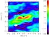 |
Fig. 1 Integrated intensity map of the H2CO 9(1, 8)–8(1, 7) emission. The color bar gives the flux scale in mJy beam-1 km s-1. The white contours indicate the 690 GHz continuum at 3, 30, and 300σ from the thermal emission of the millimeter-sized dust grains. The position of the star IRS 48 is indicated by the star and the 60 AU radius (the dust trap radius) by a white dashed ellipse. |
3. Results
The H2CO 9(1, 8)–8(1, 7) line was detected at 3−8σ levels in the channels between vLSR = −0.5 and +9.5 km s-1 (the source velocity is 4.55 km s-1, van der Marel et al. 2013). The integrated flux between −0.5 and +9.5 km s-1 shows a flattened structure centered just south of the star (Fig. 1). The stellar position (Table 1) was determined from the fastest velocity channels where the 12CO emission from the same data set was detected. The emission is extended across the spatial region, corresponding to a rectangle [−1.0′′ to +1.0′′, −0.3′′ to +0.2′′] having an area of 2.1 × 10⁻¹¹ sr. Across this area, the integrated flux is found to be ~3.1 ± 0.6 Jy km s-1 (see Figs. 1 and 2). The emission is, where detected, cospatial with the 12CO 6−5 emission at the same velocity channels, although the northern half of the emission is missing (see Fig. 3). Gas orbiting a star in principle follows Kepler’s laws, with the velocity v depending on the orbital radius r according to  , with G the gravitational constant and M the stellar mass. The CO 6–5 emission is found to follow Keplerian motion in an axisymmetric disk (Bruderer et al. 2014). The emission in the high-velocity channels is significantly stronger than the velocities closer to the source velocity, which can be partly explained by limb brightening due to the 50° inclination of the disk. Some H2CO and CO emission is found in various channels in the southeast corner (at velocities of +1−2 km s-1) and not follow the Keplerian motion pattern (Bruderer et al. 2014), but because of the low S/N it is not possible to distinguish whether this emission is real or a cleaning artifact for the case of H2CO.
A striking aspect of these images is that H2CO is only detected south of the star, as is also found for the submillimeter continuum, which shows a north-south asymmetry of the disk with a contrast factor of >100. The north-south contrast of H2CO can only be constrained to be a factor >2 because of the low S/N of this detection. Moreover, the H2CO does not follow the submillimeter continuum exactly: at the continuum peak no H2CO emission is detected at all. The velocity channels in 12CO between 2.5 and 4.5 km s-1 suffer from absorption by foreground clouds, but the H2CO abundance and excitation in these clouds is too low to absorb the H2CO disk emission in this highly excited line. Thus, the absence of H2CO at the peak millimeter continuum is significant.
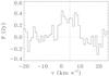 |
Fig. 2 Spectrum of H2CO 9(1, 8)−8(1, 7) toward IRS 48 spatially integrated over the rectangle [−1.0′′ to +1.0′′, −0.3′′ to +0.2′′]. The dotted line indicates the zero-emission line and the dashed line the source velocity of 4.55 km s-1. |
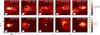 |
Fig. 3 Comparison of channel maps H2CO 9(1, 8)–8(1, 7) (top row) with 12CO 6−5 (bottom row) (data taken from Bruderer et al. 2014). The color bar indicates the fluxes in mJy beam-1. The number in the upper right corner of each map is the velocity range of that map. In the H2CO maps, the white contours indicate the 20%, 40%, 60%, 80%, and 100% of the peak intensity of all channels (the peak intensity is 195 mJy beam-1). The dashed ellipse indicates the 60 AU radius ring. The CO +4−+6 km s-1 channels are affected by foreground absorption. |
The other targeted molecules remain undetected, but the non-detection provides 3σ upper limits that can be used in the models. For the 25 mJy beam-1 km s-1 rms level, we estimated the upper limit on the total flux of CH3OH as follows: for the H2CO detected emission, the total surface area dΩ with emission > 3σ is ~1.3 × 10⁻¹¹ sr or ~7 beams, and the detectable emission lies between −0.5 and +9.5 km s-1 (11 channels). The 3σ upper limit on the total flux is thus  (1)where the factor 1.2 is introduced to compensate for small-scale noise variations and calibration uncertainties at this high frequency of the observations. Note that this is a conservative limit because the H2CO emission is most likely narrower in the radial direction than the spatial resolution. For the CN, H13CO+, and other molecules in Table 1 we expect the emission to be cospatial with the CO emission, which covers ~4.8 × 10⁻¹¹ sr or ~26 beams and integrated between −3 and +12 km s-1. The upper limit is thus
  (2)
(2)
4. Model
4.1. Physical structure
Analysis of the abundance and spatial distribution of the H2CO in the disk requires a physical model of the temperature and gas density as a function of radius and height in the disk. We used the best-fitting model of the gas structure from Bruderer et al. (2014) based on the 12CO and C17O 6−5 lines from the same ALMA data set and the dust continuum. The proper interpretation of the gas disk seen in 12CO 6−5 emission requires a thermo-chemical disk model, in which the heating-cooling balance of the gas and chemistry are solved simultaneously to determine the gas temperature and molecular abundances at each position in the disk. Moreover, even though the densities in disks are high, the excitation of the rotational levels may not be in thermodynamic equilibrium, and there are steep temperature gradients in both radial and vertical directions in the disk. The DALI model (Bruderer et al. 2012; Bruderer 2013) uses a combination of a stellar photosphere with a disk density distribution as input. For IRS 48, the stellar photosphere is represented by a blackbody of 10 000 K. It solves for the dust temperatures through continuum radiative transfer from UV to millimeter wavelengths and calculates the chemical abundances, the molecular excitation, and the thermal balance of the gas. It was developed for the analysis of the gas emission structures such as are found for transitional disks (Bruderer 2013).
DALI uses a reaction network described in detail in Bruderer et al. (2012) and Bruderer (2013). It is based on a subset of the UMIST 2006 gas-phase network (Woodall et al. 2007). About 110 species and 1500 reactions are included. In addition to the gas-phase reactions, some basic grain-surface reactions (freeze-out, thermal and nonthermal evaporation and hydrogenation like g:O → g:OH → g:H2O and H2/CH+ formation on PAHs) are included. The g:X notation refers to atoms and molecules on the grain surface. The photodissociation rates are obtained from the wavelength-dependent cross-sections by van Dishoeck et al. (2006). The adopted cosmic-ray ionization rate is ζ = 5 × 10-17 s-1. X-ray ionization and the effect of vibrationally exited H2 are also included in the network. The model chemistry output will be used to compare with the HCO+ and CN data. However, since no extensive grain-surface chemistry is included, it is not suitable to model the H2CO and CH3OH chemistry.
The surface density profile for the best-fitting model for IRS 48 (Bruderer et al. 2014) including the gap is shown in Fig. 4. It is found that the gas disk around IRS 48 has a very low mass (1.4 × 10⁻⁴ M⊙ = 0.15 MJup) compared with the mean disk mass of ~5 MJup for normal disks (Williams & Cieza 2011; Andrews et al. 2013). Furthermore, the disk has a large scale-height, allowing a large portion of the inner walls to be irradiated by the star. The radial gas structure has two density drops: a drop δ20 of <10-1 in the inner 20 AU (probably caused by a planetary or substellar companion) and an additional drop δ60 of 10-1 at 60 AU radius.
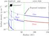 |
Fig. 4 Adopted radial density structure of the IRS 48 disk, taken from Bruderer (2013). The blue lines indicate the gas surface density, the red lines the dust surface density. The dotted black lines show the undisturbed surface density profiles if it continued from outside inwards without depletion. The green dashed lines indicate the radii at which the depletions start. |
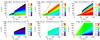 |
Fig. 5 Physical-chemical model of IRS 48 from Bruderer et al. (2014). The panels show gas density (cm-3), gas temperature (K), CO abundance with respect to H2, dust density (cm-3), dust temperature (K), and UV field in G0 (G0 = 1 refers to the standard interstellar radiation field). The given numbers are in 10log scale. |
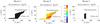 |
Fig. 6 Trial abundance models 1, 2 and 3 for H2CO. The H2CO abundance is limited by photodissociation in the upper layer and freeze out below 60 K. Model 1 assumes a constant abundance, model 2 assumes a fractional abundance with respect to CO, model 3 assumes a constant abundance in between 60 and 70 AU radius and zero abundance at other radii. |
The resulting densities, temperatures and CO abundances of the model are given in Fig. 5. The gas density is 105−6 molecules cm-3 in the upper layers of the disk, increasing to 108 cm-3 close to the midplane near 60 AU. The gas temperature is typically a few 100 K, except in the upper layers where the temperature reaches several thousand K. The UV radiation field is enhanced by factors of up to 108 in the disk, indicated by G0 (panel 6 in Fig. 5). G0 = 1 refers to the interstellar radiation field defined as in Draine (1978), ~2.7 × 10⁻³ erg s-1 cm-2 with photon-energies in the far UV range between 6 eV and 13.6 eV. The CO abundance is ~10-4 compared with H2 throughout the bulk of the outer disk and is not frozen out.
The H2CO emission was modeled using the LIne Modeling Engine (LIME), a non-LTE excitation spectral line radiation transfer code (Brinch & Hogerheijde 2010). The physical structure described above is used as input. The first step in the analysis is to empirically constrain the H2CO abundance by using three different trial abundance profiles guided by astrochemical considerations. The inferred abundances were then a posteriori compared with those found in the full chemical models. In model 1, the abundance was assumed to be constant throughout the disk, testing abundances between 10-5 and 10-11 with respect to H2. In model 2, the abundance was taken to follow the CO abundance calculated by the DALI model, taking a fractional abundance ranging between 10-3 and 10-8 with respect to CO. Model 3 was inspired by Cleeves et al. (2011) by setting the H2CO to zero except for a ring between 60 and 70 AU. This model assumes that the UV irradiated inner rim has an increased chemical complexity that can be observed directly, as material from the midplane has been liberated from the ices. The abundance profile is additionally constrained by the photodissociation and freeze out. H2CO can only exist below the photodissociation height, which was taken as the height (z direction) where a hydrogen column density of N(H2) = 4 × 1020 cm-2 is reached. At this column, the CO photodissociation rate drops significantly due to shielding by dust as well as self-shielding and mutual shielding by H2 for low gas-to-dust ratios (Visser et al. 2009). Therefore, at each radius this value was calculated and the abundance was set to zero above it. For radii <60 AU, H2CO is photodissociated almost entirely down to the midplane because of the lower total column density. Furthermore, H2CO is expected to be frozen out on the grains at temperatures <60 K since it has a higher binding energy (Ioppolo et al. 2011) than CO, therefore the abundance in regions below this temperature were also set to zero. All three abundance profiles are shown in Fig. 6.
The LIME grid was built using linear sampling, with the highest grid density starting at 60 AU, using 30 000 grid points and 12 000 surface grid points, using an outer radius of 200 AU. The image cubes were calculated for 60 velocity channels of width 0.5 km s-1 spectral resolution, in 5′′ × 5′′ maps with 0.025′′ pixels. Collisional rate coefficients were taken from the Leiden Atomic and Molecular Database (LAMDA; Schöier et al. 2005) with references to the original collisional rate coefficients as follows: H2CO (Troscompt et al. 2009), CH3OH (Rabli & Flower 2010), H13CO+ (Flower 1999), and CN (Lique et al. 2010). For the other molecules the emission was only calculated in LTE, using the parameters from CDMS (Müller et al. 2001, 2005).
For CH3OH, H13CO+, CN and the other molecules we ran models to constrain the upper limits. For CH3OH, the same abundance profiles as for H2CO were taken because CH3OH is expected to be cospatial with H2CO when they are both formed through solid-state chemistry. For the H13CO+ abundance the initial CO abundance was taken and multiplied with factors 10-5–10-11, as the HCO+ is known to form via CO through the H + CO proton donation reaction and is indeed observed to be strongly correlated with CO (Jørgensen et al. 2004). For the other molecules the same approach for the abundance as for H13CO+ was used.
4.2. Results
The model results for H2CO are presented in Fig. 7. Integrated fluxes were computed by summing the model fluxes over the same rectangular region as the H2CO observations, after subtracting the continuum. Figure 7 presents the model fluxes as a function of H2CO abundance for the three trial abundance structures. Model 1 with constant H2CO abundance ~10−8 ± 0.15 with respect to H2 or model 2 with abundance ~10-4 with respect to CO reproduce the total observed flux well within the error bar. There is little difference between model 1 and model 2 except for a factor of 104 that has been taken into account in Fig. 7. This is expected because most of the CO abundance in the defined region is 10-4 with respect to H2. Model 3 requires an abundance of 10-8 higher by a factor 3 in the 60−70 AU ring to give the same integrated flux. Note that the LIME model fluxes obtained with non-LTE calculations are only about 25% lower than the LIME models in LTE due to the high densities in the disk.
The spectra (Fig. 8) confirm that the best match for the flux for model 1 is for an abundance of ~10-8, although the peaks at the highest velocities are up to twice as high as the data. The slight asymmetry in these model spectra is caused by the spatial integration over a rectangle, whereas the disk has a position angle of 96°. The line wings in models 1 and 2 originate from the emission from radii <60 AU, which is missing in model 3, but the S/N of the data is too low to detect the difference. In the bottom panel of Fig. 8 the spectra have been scaled so that the total flux exactly matches that from the observations.The current models underproduce the emission close to the central velocity ratios, suggesting that the abundance may be even more enhanced in the central southern part of the disk at these velocities and is not constant along the azimuthal direction of the semi-ring. It is also possible that there is enhanced H2CO at larger radii than assumed here when the freeze-out zone is taken out, although this does not add a significant amount of emission at the central velocities. Calculation of an abundance model where the freeze-out zone is removed shows that this indeed increases the emission at central velocities, but the S/N of the data is insufficient to confirm or exclude emission at larger radii. Overall, it is concluded that the abundance is ~10-8 compared with H2 within factors of a few.
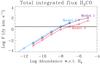 |
Fig. 7 Results of H2CO abundance models: total flux integrated over the emission rectangle of the observations for different abundances for model 1 (purple), model 2 (blue), and model 3 (red). The fractional abundances with respect to CO for model 2 have been multiplied with 10-4 for easier comparison as the CO/H2 abundance is typically 10-4. The dotted line indicates the measured observed flux, and the gray bar indicates the error on this value based on the flux calibration uncertainty. |
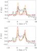 |
Fig. 8 Results of H2CO abundance models: spectra integrated over the emission rectangle of the observations for different abundances for model 1 (purple), model 2 (green), and model 3 (red) for abundances 10-7 (dashed), 10-8 (solid), and 10-9 (dotted). The black spectrum represents the observational data. Abundances for model 2 are multiplied with 10-4 to translate the abundance w.r.t. CO to H2. The top figure shows the original models. The bottom figure shows the model spectra scaled to match the total flux of the observations. |
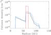 |
Fig. 9 Column density profiles of H2CO for the best abundance fits for models 1 (black), 2 (blue), and 3 (red). Abundances are 10-8 for model 1, 10-4 w.r.t. CO for model 2 and 10-7 for model 3. |
The final comparison between models and data is made by comparing images. To produce images from the model output cubes the images were convolved with the ALMA beam of the observations (0.31′′ × 0.21′′, PA 96°). Similar as in Bruderer et al. (2014), the result of the model images convolved to the ALMA beam was compared with the result of simulated ALMA observations. An alternative method is to convert the model images to (u, v)-data according to the observed (u, v)-spacing using the CASA software and reduce them in the same way as the observations. Because of the good (u, v)-coverage of our observations, the two approaches do not differ measurably within the uncertainty errors. Figures 10 and 11 indicate that the three models have a similar ring-like structure as the observations, apart from the emission in the north that is lacking in the data. The differences between the models are best seen in the velocity channel maps: models 1 and 2 still show some emission within the ring at 30–60 AU, which is higher for model 1 than for model 2 because the CO abundance is somewhat lower between 40 and 60 AU. Model 3 does not show any emission within the ring by design.
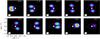 |
Fig. 10 Results of H2CO abundance modeling: channelmap convolved with the ALMA beam of the observations for Model 1 at 10-8 abundance. The 60 AU radius is indicated with a dashed ellipse and the stellar position with a star. The white contours indicate the 20%, 40%, 60%, 80% and 100% of the peak (peak is 212 mJy beam-1). |
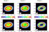 |
Fig. 11 Results of H2CO abundance models: integrated intensity maps convolved with the ALMA beam for Model 1 at 10-8 abundance (left), Model 2 at 10-4 fractional abundance of CO (center) and Model 3 at 10-8 abundance (right). The color bar gives the flux scale in mJy beam-1. The white contours indicate the 20%, 40%, 60%, 80% and 100% of the peak. The top panel gives the result for the non-altered model image, the bottom panel gives the result with a correction for the continuum extinction. |
A possible explanation for the missing H2CO emission at the peak of the dust continuum is that the dust is not entirely optically thin. The optical depth τd was calculated as τd ~ 0.43 (van der Marel et al. 2013) averaged over the continuum region. If we assume all the H2CO emission Iline to originate from behind the dust, the resulting intensity is  (3)The first term is the measured dust intensity, which is subtracted from the H2CO data. The second term indicates a reduction of the line intensity by continuum extinction. This extinction was calculated by multiplying the model output with the exponent of a 2D τd profile, where τd is following the continuum emission profile of the observed dust trap area. The maximum τd was taken as 0.86, recovering the averaged opacity over this area. This correction represents an upper limit of the continuum extinction effect. The result is shown in the bottom panels of Fig. 11. The continuum extinction decreases the H2CO emission in the south by more than a factor 2, while some emission between the star and the dust continuum remains (for models 1 and 2). Although the strength of this emission compared with the peaks at the edges is still lower than in the observations, the model image is now more consistent with the observations. The total integrated flux is only 10% lower because the rectangle used for the spatial integration did not cover most of the dust continuum. Both the S/N of the line data and the unknown mixing of the gas and dust prevent a more detailed analysis of this problem, but it is clear that the continuum extinction cannot be neglected. The observations show a decrease of a factor 4 between the east and west limbs compared with the emission at the location of the dust peak (see Fig. 1), which requires a τd of at least 1.4. Submillimeter imaging at longer wavelengths is required to measure the dust optical depth more accurately.
Overall, the conclusion is that the current data can constrain the H2CO abundance in the warm gas where H2CO is thought to reside to ~10-8, but the current S/N is too low to distinguish the different assumptions on the radial distribution of H2CO. However, the three models make different predictions for the distribution, which we expect to see more clearly in future higher S/N ALMA data.
The total model fluxes for the CH3OH, H13CO+ and CN are compared with the derived upper limits in Fig. 12, where all abundances have been multiplied with 10-4 to translate the abundance w.r.t. CO to H2. The other targeted molecules with upper limits were compared in the same way (plots not displayed here). For the CH3OH lines, the upper limit on the integrated flux is consistent with an abundance limit in model 1 of <3 × 10⁻⁸, thus H2CO/CH3OH > 0.3. For H13CO+, the upper limit sets the abundance at <10-6 with respect to CO. This indicates an HCO+/CO abundance ratio of <10-4, or an absolute abundance HCO+/H2 of <10-8. The CN emission is poorly constrained: the upper limit sets the CN/CO abundance at <5 × 10⁻⁴ or CN/H2 < 5 × 10⁻⁸. The reason is the low Einstein A coefficient of this particular transition, which is almost three orders of magnitude lower than that of the other transitions in this study.
Derived abundance limits w.r.t. H2.
All derived absolute abundance limits are given in Table 2. For 34SO2 and C34S we found absolute abundances of <10-8 and <10-9 respectively, corresponding to abundances of <2 × 10⁻⁷ and <2 × 10⁻⁸ for the main isotopes, assuming an elemental abundance ratio of sulfur of 32S/34S of 24 (Wilson & Rood 1994). For the deuterated molecules N2D+ and D2O the isotope ratio D/H in these molecules is not known, therefore no upper limits on N2H+ or H2O can be obtained.
5. Discussion
5.1. Origin of the H2CO emission
H2CO can be formed efficiently in the ice phase by hydrogenation of solid CO, as shown in laboratory experiments, which can be followed by the formation of CH3OH (Hiraoka et al. 2002; Watanabe & Kouchi 2002; Watanabe et al. 2004; Hidaka et al. 2004; Fuchs et al. 2009):  (4)Because CO ice is highly abundant in the cold dusty regions in clouds and disks, this formation route is commonly assumed as the origin of gas-phase H2CO, following thermal or nonthermal desorption. In that case, CH3OH is expected to have a similar or higher abundance than H2CO because they are formed along the same sequence (Tielens & Hagen 1982; van der Tak et al. 2000; Cuppen et al. 2009). If all ices are thermally desorbed, gas-phase abundances can be as high as ~10-6 − 10-5.
There is no known efficient gas-phase chemistry for the formation of CH3OH (Geppert et al. 2006; Garrod et al. 2006), whereas H2CO can also be formed rather efficiently in the gas phase. At low temperatures, the reaction  (5)dominates its formation, whereas it is mainly destroyed through reactions with ions such as HCO+and H3O+. These reactions lead to H3CO+, which cycles back to H2CO through dissociative recombination
  (6)However, since the branching ratio to H2CO is only 0.3 (Hamberg et al. 2007), the ion reactions lead to a net destruction of H2CO. Typical dark-cloud gas-phase model abundances are a few × 10-8 relative to H2 (McElroy et al. 2013). At low dust temperatures (<60 K), H2CO can freeze out after formation.
At higher temperatures in the presence of abundant H2O (T > 100 K), formaldehyde can also form through gas-phase reactions such as CH +H2O → H3CO+ + H followed by dissociative recombination. Above a few 100 K, formaldehyde is destroyed efficiently through H + H2CO + 1380 K → HCO + H2.
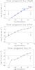 |
Fig. 12 Model results for the integrated fluxes found for CH3OH, H13CO+ and CN in the empirical models. The dashed line indicates the upper limit of the integrated intensity, assuming the molecule is cospatial with the H2CO (CH3OH) or CO (H13CO+ and CN). Abundances were calculated with respect to the CO abundance, but in these plots are multiplied with 10-4 to translate the abundance w.r.t. CO to H2. |
H2CO has been detected in warm protostellar cores together with CH3OH. Typical H2CO abundances in the warm gas are 3 ~ 10-7 with respect to hydrogen, whereas CH3OH has an abundance higher by a factor of 5 (H2CO/CH3OH ≈ 0.2) (Bisschop et al. 2007), suggesting a main formation route through solid-state chemistry followed by sublimation. Recent observations of these molecules in the Horsehead PDR and core show a higher abundance ratio H2CO/CH3OH of 1−2, which cannot be produced by pure gas-phase chemistry (Guzmán et al. 2013). H2CO has been detected in several protoplanetary disks (Dutrey et al. 1997; Aikawa et al. 2003; Thi et al. 2004; Öberg et al. 2010, 2011; Qi et al. 2013a), which has usually been interpreted through the solid state chemical path, even though gas-phase CH3OH has not been detected in any of these disks due to sensitivity limitations. For high enough sensitivity the combination of H2CO and CH3OH observations would clearly distinguish between the ice-phase and gas-phase chemistry. For the disk around HD 163296, the rotational temperature of H2CO was measured to be <30 K by fitting the emission of several transitions, and its abundance was found to be enhanced outside the CO “snowline” at 20 K, suggesting a solid-state route (Qi et al. 2013a).
The measured H2CO/CH3OH ratio limit for Oph IRS 48 of >0.3 is similar to the limit found for LkCa 15 (Thi et al. 2004) and only slightly higher than that found in warm protostars. This low limit therefore does not exclude the solid-state chemistry formation route but is also consistent with a gas-phase chemistry contribution to H2CO. However, the H2CO abundance of 10-8 is much higher than the detections and upper limits of the disk-averaged abundances in Thi et al. (2004), which are typically <10-11. Most of this difference stems from the fact that the disks in Thi et al. (2004) are two orders of magnitude more massive and also colder, with a large portion of the CO and related molecules frozen out. This cold zone is lacking in the IRS 48 disk, and our analysis has already removed the zones in which H2CO is photodissociated or frozen out. Nevertheless, as shown below, the H2CO emission is unusually strong in IRS 48 for its disk mass, hinting at an increased richness of chemistry in transitional disks due to the directly irradiated inner rim at the edge of the gas gap, as predicted (Cleeves et al. 2011).
Another interesting aspect of the H2CO emission is the azimuthal asymmetry in IRS 48, which happens to be similar although not exactly cospatial to the dust continuum asymmetry. The dust asymmetry was modeled (van der Marel et al. 2013) as a dust trap caused by a vortex in the gas distribution with an overdensity of a factor 3, and it is possible that the increased emission of H2CO at this location is in fact tracing this overdensity in the gas. The image quality and S/N of the observations is insufficient to confirm this claim, however, and no overdensity was observed in the 12CO 6−5 emission (Bruderer et al. 2014). Moreover, the H2CO emission does not peak exactly at the peak of the dust continuum emission: in fact, the H2CO emission is decreased at the continuum peak, as discussed in Sect. 4.2 (see Fig. 1). It is possible that this decrease is caused by the high optical depth of the millimeter dust, which absorbs the line emission of the optically thin gas all the way from the midplane (see Fig. 11 and Eq. (3)). This cannot be confirmed because of the unknown vertical mixing of the gas and dust. Finally, a nondetection of an overdensity in the gas is consistent with the dust-trapping scenario: a vortex in the gas may already have disappeared while the created dust asymmetry remains because the time scale of smoothing out a dust asymmetry is on the order of several Myr (Birnstiel et al. 2013).
Another possibility for the increased H2CO emission in the south is a local decrease in the temperature compared with the north. In that case H2CO is destroyed efficiently in the north through the H + H2CO + 1380 K → HCO + H2 reaction, but not in the south. This possibility is consistent with the reduced CO emission in the south in both the rovibrational lines (Brown et al. 2012) and the 12CO 6−5 lines (Bruderer et al. 2014), where Bruderer et al. (2014) suggested the temperature decrease to be of a factor 3. This temperature decrease might be caused by UV shielding in the inner disk. Note that the millimeter dust that is concentrated in the south does not provide sufficient cooling to change the gas temperature significantly through gas-grain collisions: the small dust grains have most the surface and gas-grain temperature exchange. If the temperature drops locally to between 20 and 30 K, the H2CO might even be an ice-phase product, but this is very unlikely. A final possibility is that the increase of H2CO is caused by the increased dust density and dust collisions in this region. If the grain-grain collisions are at high enough speed (which depends on the turbulence in the disk), the ice molecules may become separated from the grains. However, the dust grains have reached temperatures above the sublimation temperature of 60 K long before reaching the dust trap, therefore this is not very likely within reasonable time scales.
5.2. Comparison with chemical models
The column density of H2CO for the best-fitting model with abundance 10-8 is ~1014 cm-2 for radii > 60 AU (Fig. 9), which is within an order of magnitude of the predictions of chemical models (Semenov & Wiebe 2011; Walsh et al. 2012, 2013) for protoplanetary disks. For the 10-7.5 abundance upper limit for CH3OH we found a column density limit of ~2−4 × 1014 cm-2 for radii > 60 AU, which is well above the numbers derived in chemical models (Walsh et al. 2012; Vasyunin et al. 2011), which are typically 1010 cm-2.
The DALI-model (Bruderer et al. 2014) produces predictions for HCO+ and CN: the HCO+ abundance peaks at 5 × 10⁻⁹, but only in a very thin upper layer of the disk where the CO + H2 reaction operates. The disk-averaged abundance is much lower. The predicted integrated model intensity for H13CO+ is 0.02 Jy km s-1, far below our detection limit of 1.8 Jy km s-1. The peak abundance for CN is 3 × 10⁻⁷ with an integrated intensity of 1.1 Jy km s-1, which is close to our upper limit. The other CN 6−5 lines at 680 GHz (outside the range of the spectral window of our observations) have an Einstein coefficient that is 2 orders of magnitude higher and should be readily detectable with an integrated flux of 15 Jy km s-1.
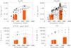 |
Fig. 13 Model predictions for the integrated fluxes for H2CO (both ortho and para lines, assuming an ortho/para ratio of 3), and upper limits for A-CH3OH, H13CO+, HCO+ (triangles and diamonds, respectively), and CN based on our best-fit models for detections and upper limits. The boxes show the 3σ upper limit of the ALMA sensitivity for Band 6 (230 GHz), Band 7 (345 GHz), and Band 9 (690 GHz), integrated over the line profile for one hour integration in the full array. The targeted lines in observations are indicated in red (this study), blue (Öberg et al. 2010, 2011), and purple (Thi et al. 2004). The lines that have the best potential for observation compared with the ALMA sensitivity are encircled. |
5.3. Comparison of upper limits with other observations
The HCO+/CO ratio of <10-4 (or HCO+/H2 < 10-8) for IRS 48 is consistent with values found in disks, protostellar regions and dark clouds. The ratio is often found to be ≥10-5, where the lower limit is due to the unknown optical depth of the observed HCO+ line (Thi et al. 2004). Our H13CO+ line does not suffer from this problem, but our inferred HCO+ abundance is not more stringent because of the very low gas mass of IRS 48. For similar abundances, all measured fluxes would be a factor of 10–100 lower than for other full disks.
HCO+ is produced by the gas-phase reaction H + CO → HCO+ + H2, which relates the abundance directly to ionization, because the parent molecule H is formed efficiently through cosmic-ray ionization. Our abundance cannot set a strong limit on the ionization fraction in the disk. The ionization fraction in disks is important because the magneto-rotational instability (MRI), believed to drive viscous accretion, requires ionization to couple the magnetic field to the gas (Gammie 1996). Insufficient ionization may suppress the MRI and create a so-called dead zone that can create dust traps at its edge where the dust grains will gather (Regály et al. 2012). However, the ionization needs to be lower than about 10-12 to induce a dead zone (Ilgner & Nelson 2006). On the other hand, recent models suggest that cosmic rays may be excluded altogether from disks around slightly lower-mass stars (Cleeves et al. 2013). A detection of HCO+ at the level suggested by our models would provide direct proof of the presence of cosmic rays that ionize H2 at a rate of ~5 × 10-17 s-1.
The CN upper limit is difficult to compare with literature values because our upper limit is very high due to the low Einstein A coefficient. Literature values give derived abundances (Thi et al. 2004) of ~10-10, three orders of magnitude lower than our upper limit, which is again caused by the low gas mass of our disk. As noted above, the full chemical model by Bruderer (2013) suggests abundances very close to our inferred upper limits. The CN/HCN ratio is a related tracer for photodissociation in the upper layers and at the rim of the outer disk: a high ratio indicates a strong UV field, since CN is produced by radical reactions with atomic C and N (in the upper layers) and by photodissociation of HCN, whereas CN cannot easily be photodissociated itself (Bergin et al. 2003; van Dishoeck et al. 2006). The CN/HCN ratio is generally found to be higher in disks around the hotter Herbig stars. HCN observations are required to measure this ratio for IRS 48.
Several of the other targeted molecules have been detected towards cores and protostars, such as 34SO2 (Persson et al. 2012), N2D+ (Emprechtinger et al. 2009) and HNCO (Bisschop et al. 2007). N2D+ can be used as a deuteration tracer in combination with N2H+, and therefore a tracer of temperature evolution, but this line was not within our spectral setup. The H2CO/HNCO abundance limit of >0.3 as derived for IRS 48 is rather conservative compared with values in cores of ~10 (Bisschop et al. 2007), but the N-bearing molecules are weak in IRS 48. The c-C3H2 molecule was recently detected for the first time in the HD 163296 disk (Qi et al. 2013b), and their derived column density of ~1012 cm-2 is well below our observed limit for IRS 48 of 1013 cm-2.
5.4. Predictions of line strengths of other transitions
Most observations of molecules in disks present only intensities, but do not derive abundances, since a physical disk model is generally not available. To compare our observations with these data, we calculated the expected disk-integrated fluxes for other transitions, using our physical model and derived abundances or upper limits. These results are presented in Fig. 13. The ALMA sensitivity limits for Band 6, Band 7, and Band 9 (230, 345 and 690 GHz) for the ALMA full array of 54 antennas for 1 h integration are included to investigate which lines provide the best constraints for future observations.
Figure 13 shows the potential for future observations of IRS 48, indicating that with full ALMA much better upper limits or detections can be reached for all of these species in just one hour of integration by choosing the correct lines. The H2CO flux can be measured with much better S/N and there is a wide range of abundances that can be tested. Lines in Band 7 (345 GHz) generally have the highest potential.
For H2CO, lines that have been targeted most often are the para H2CO 3(0, 3)−2(0, 2) and 3(2, 2)−2(2, 1) transitions at 218.22 and 218.47 GHz, as well as the ortho-H2CO 4(1, 4)−3(1, 3) line at 281.53 GHz (Öberg et al. 2010, 2011). Comparing the observed fluxes with our predictions for these lines (~0.3 Jy km s-1) shows that the H2CO emission of IRS 48 is quite similar to that found in other disks. This is remarkable because of the low disk mass of IRS 48.
CH3OH has not been detected in other disks to date. Upper limits derived for a few disks (Thi et al. 2004) give abundances <10-10, below our limits for IRS 48. The fact that our observed H2CO fluxes are similar to those of other disks in spite of the low disk mass bodes well for future studies. Targeted ALMA observations of the strongest lines will allow much better sensitivity and are expected to easily reduce the abundance limits by 1−2 orders of magnitude. Together with searches for other complex organic molecules made preferentially in the ice, this will allow direct tests of the mechanism of sublimation of mid-plane ices in transitional disks proposed by Cleeves et al. (2011).
6. Conclusions
We observed the Oph IRS 48 protoplanetary disk with ALMA Early Science at the highest frequencies, around 690 GHz, allowing the detection of warm H2CO and upper limits on the abundances of several other molecules including CH3OH, H13CO+, and CN lines at unprecedented angular resolution.
-
1.
We detected and spatially resolved the warm H2CO 9(1, 8)−8(1, 7) line, which reveals a semi-ring of emission at ~60 AU radius centered south from the star. No emission is detected in the north. This demonstrates that H2CO, an ingredient for building more complex organic molecules, is present in a location of the disk where planetesimals and comets are currently being formed.
-
2.
The H2CO emission was modeled using a physical disk model based on the dust continuum and CO emission (Bruderer et al. 2014), using three different trial abundance profiles. None of the profiles were able to match the observed data exactly, but the absolute flux indicates an abundance with respect to H2 of ~10-8.
-
3.
The combination of the H2CO abundance in combination with upper limits for the CH3OH emission indicates a H2CO/CH3OH ratio >0.3. This limit together with the overall abundance suggests that both solid-state and gas-phase processes occur in the disk.
-
4.
Although the H2CO emission is located only on the southern side of the disk, just like the millimeter dust continuum, the offset with the continuum peak and the low S/N do not allow a firm claim on a relation with the dust-trapping mechanism.
-
5.
The upper limit for H13CO+ indicates an HCO+ abundance of < 10-8, consistent with our model. The upper limit for CN of 10-7.3 relative to H2 is directly at the level of that predicted by our model. Upper limits on the abundances of the other targeted molecules are consistent with earlier observations.
-
6.
Future ALMA observations of intrinsically stronger lines will allow abundances to be measured that are one or more orders of magnitude below the upper limits derived here. This will allow full tests of the chemistry of simple and more complex molecules in transitional disks.
Acknowledgments
The authors would like to thank C. Walsh for useful discussions and M. Schmalzl for help with the observational setup. N.M. is supported by the Netherlands Research School for Astronomy (NOVA), T.v.K. by the Dutch ALMA Regional Center Allegro financed by Netherlands Organization for Scientific Research (NWO) and S.B. acknowledges a stipend by the Max Planck Society. Astrochemistry in Leiden is supported by the Netherlands Research School for Astronomy (NOVA), by a Royal Netherlands Academy of Arts and Sciences (KNAW) professor prize, and by the European Union A-ERC grant 291141 CHEMPLAN. This paper makes use of the following ALMA data: ADS/JAO.ALMA#2011.0.00635.S. ALMA is a partnership of ESO (representing its member states), NSF (USA) and NINS (Japan), together with NRC (Canada) and NSC and ASIAA (Taiwan), in cooperation with the Republic of Chile. The Joint ALMA Observatory is operated by ESO, AUI/NRAO and NAOJ.
References
- Aikawa, Y., Momose, M., Thi, W.-F., et al. 2003, PASJ, 55, 11 [NASA ADS] [CrossRef] [Google Scholar]
- Andrews, S. M., Rosenfeld, K. A., Kraus, A. L., & Wilner, D. J. 2013, ApJ, 771, 129 [NASA ADS] [CrossRef] [Google Scholar]
- Bergin, E., Calvet, N., D’Alessio, P., & Herczeg, G. J. 2003, ApJ, 591, L159 [NASA ADS] [CrossRef] [Google Scholar]
- Bergin, E. A., Aikawa, Y., Blake, G. A., & van Dishoeck, E. F. 2007, Protostars and Planets V, 751 [Google Scholar]
- Birnstiel, T., Dullemond, C. P., & Pinilla, P. 2013, A&A, 550, L8 [NASA ADS] [CrossRef] [EDP Sciences] [Google Scholar]
- Bisschop, S. E., Fraser, H. J., Öberg, K. I., van Dishoeck, E. F., & Schlemmer, S. 2006, A&A, 449, 1297 [NASA ADS] [CrossRef] [EDP Sciences] [Google Scholar]
- Bisschop, S. E., Jørgensen, J. K., van Dishoeck, E. F., & de Wachter, E. B. M. 2007, A&A, 465, 913 [NASA ADS] [CrossRef] [EDP Sciences] [Google Scholar]
- Brinch, C., & Hogerheijde, M. R. 2010, A&A, 523, A25 [NASA ADS] [CrossRef] [EDP Sciences] [Google Scholar]
- Brown, J. M., Herczeg, G. J., Pontoppidan, K. M., & van Dishoeck, E. F. 2012, ApJ, 744, 116 [NASA ADS] [CrossRef] [Google Scholar]
- Bruderer, S. 2013, A&A, 559, A46 [NASA ADS] [CrossRef] [EDP Sciences] [Google Scholar]
- Bruderer, S., van Dishoeck, E. F., Doty, S. D., & Herczeg, G. J. 2012, A&A, 541, A91 [NASA ADS] [CrossRef] [EDP Sciences] [Google Scholar]
- Bruderer, S., van der Marel, N., van Dishoeck, E. F., & van Kempen, T. A. 2014, A&A, 562, A26 [NASA ADS] [CrossRef] [EDP Sciences] [Google Scholar]
- Casassus, S., van der Plas, G. M. S. P., et al. 2013, Nature, 493, 191 [NASA ADS] [CrossRef] [Google Scholar]
- Ceccarelli, C., Loinard, L., Castets, A., Tielens, A. G. G. M., & Caux, E. 2000, A&A, 357, L9 [NASA ADS] [Google Scholar]
- Cleeves, L. I., Bergin, E. A., Bethell, T. J., et al. 2011, ApJ, 743, L2 [NASA ADS] [CrossRef] [Google Scholar]
- Cleeves, L. I., Adams, F. C., & Bergin, E. A. 2013, ApJ, 772, 5 [NASA ADS] [CrossRef] [Google Scholar]
- Collings, M. P., Anderson, M. A., Chen, R., et al. 2004, MNRAS, 354, 1133 [NASA ADS] [CrossRef] [Google Scholar]
- Cuppen, H. M., van Dishoeck, E. F., Herbst, E., & Tielens, A. G. G. M. 2009, A&A, 508, 275 [NASA ADS] [CrossRef] [EDP Sciences] [Google Scholar]
- Draine, B. T. 1978, ApJS, 36, 595 [NASA ADS] [CrossRef] [Google Scholar]
- Dutrey, A., Guilloteau, S., & Guelin, M. 1997, A&A, 317, L55 [NASA ADS] [Google Scholar]
- Ehrenfreund, P., & Charnley, S. B. 2000, ARA&A, 38, 427 [Google Scholar]
- Emprechtinger, M., Caselli, P., Volgenau, N. H., Stutzki, J., & Wiedner, M. C. 2009, A&A, 493, 89 [NASA ADS] [CrossRef] [EDP Sciences] [Google Scholar]
- Flower, D. R. 1999, MNRAS, 305, 651 [NASA ADS] [CrossRef] [Google Scholar]
- Fuchs, G. W., Cuppen, H. M., Ioppolo, S., et al. 2009, A&A, 505, 629 [NASA ADS] [CrossRef] [EDP Sciences] [Google Scholar]
- Fukagawa, M., Tsukagoshi, T., Momose, M., et al. 2013, PASJ, 65, L14 [NASA ADS] [CrossRef] [Google Scholar]
- Gammie, C. F. 1996, ApJ, 457, 355 [NASA ADS] [CrossRef] [Google Scholar]
- Garrod, R., Park, I. H., Caselli, P., & Herbst, E. 2006, Faraday Discussions, 133, 51 [Google Scholar]
- Geers, V. C., Pontoppidan, K. M., van Dishoeck, E. F., et al. 2007, A&A, 469, L35 [NASA ADS] [CrossRef] [EDP Sciences] [Google Scholar]
- Geppert, W. D., Hamberg, M., Thomas, R. D., et al. 2006, Faraday Discussions, 133, 177 [Google Scholar]
- Guzmán, V. V., Goicoechea, J. R., Pety, J., et al. 2013, A&A, 560, A73 [NASA ADS] [CrossRef] [EDP Sciences] [Google Scholar]
- Hamberg, M., Geppert, W. D., Thomas, R. D., et al. 2007, Mol. Phys., 105, 899 [NASA ADS] [CrossRef] [Google Scholar]
- Henning, T., & Semenov, D. 2013, Chem. Rev., 113, 9016 [Google Scholar]
- Herbst, E., & van Dishoeck, E. F. 2009, ARA&A, 47, 427 [NASA ADS] [CrossRef] [Google Scholar]
- Hidaka, H., Watanabe, N., Shiraki, T., Nagaoka, A., & Kouchi, A. 2004, ApJ, 614, 1124 [NASA ADS] [CrossRef] [Google Scholar]
- Hiraoka, K., Sato, T., Sato, S., et al. 2002, ApJ, 577, 265 [NASA ADS] [CrossRef] [Google Scholar]
- Ilgner, M., & Nelson, R. P. 2006, A&A, 445, 205 [NASA ADS] [CrossRef] [EDP Sciences] [Google Scholar]
- Ioppolo, S., van Boheemen, Y., Cuppen, H. M., van Dishoeck, E. F., & Linnartz, H. 2011, MNRAS, 413, 2281 [NASA ADS] [CrossRef] [Google Scholar]
- Jørgensen, J. K., Schöier, F. L., & van Dishoeck, E. F. 2004, A&A, 416, 603 [NASA ADS] [CrossRef] [EDP Sciences] [Google Scholar]
- Kastner, J. H., Zuckerman, B., Hily-Blant, P., & Forveille, T. 2008, A&A, 492, 469 [NASA ADS] [CrossRef] [EDP Sciences] [Google Scholar]
- Lique, F., Spielfiedel, A., Feautrier, N., et al. 2010, J. Chem. Phys., 132, 024303 [NASA ADS] [CrossRef] [PubMed] [Google Scholar]
- McElroy, D., Walsh, C., Markwick, A. J., et al. 2013, A&A, 550, A36 [NASA ADS] [CrossRef] [EDP Sciences] [Google Scholar]
- Müller, H. S. P., Thorwirth, S., Roth, D. A., & Winnewisser, G. 2001, A&A, 370, L49 [NASA ADS] [CrossRef] [EDP Sciences] [Google Scholar]
- Müller, H. S. P., Schlöder, F., Stutzki, J., & Winnewisser, G. 2005, J. Mol. Struct., 742, 215 [NASA ADS] [CrossRef] [Google Scholar]
- Mumma, M. J., & Charnley, S. B. 2011, ARA&A, 49, 471 [NASA ADS] [CrossRef] [Google Scholar]
- Öberg, K. I., Qi, C., Fogel, J. K. J., et al. 2010, ApJ, 720, 480 [NASA ADS] [CrossRef] [Google Scholar]
- Öberg, K. I., Qi, C., Fogel, J. K. J., et al. 2011, ApJ, 734, 98 [NASA ADS] [CrossRef] [Google Scholar]
- Persson, M. V., Jørgensen, J. K., & van Dishoeck, E. F. 2012, A&A, 541, A39 [NASA ADS] [CrossRef] [EDP Sciences] [Google Scholar]
- Qi, C., Öberg, K. I., & Wilner, D. J. 2013a, ApJ, 765, 34 [NASA ADS] [CrossRef] [Google Scholar]
- Qi, C., Öberg, K. I., Wilner, D. J., & Rosenfeld, K. A. 2013b, ApJ, 765, L14 [NASA ADS] [CrossRef] [Google Scholar]
- Rabli, D., & Flower, D. R. 2010, MNRAS, 406, 95 [NASA ADS] [CrossRef] [Google Scholar]
- Regály, Z., Juhász, A., Sándor, Z., & Dullemond, C. P. 2012, MNRAS, 419, 1701 [NASA ADS] [CrossRef] [Google Scholar]
- Schöier, F. L., van der Tak, F. F. S., van Dishoeck, E. F., & Black, J. H. 2005, A&A, 432, 369 [NASA ADS] [CrossRef] [EDP Sciences] [Google Scholar]
- Semenov, D., & Wiebe, D. 2011, ApJS, 196, 25 [NASA ADS] [CrossRef] [Google Scholar]
- Thi, W.-F., van Zadelhoff, G.-J., & van Dishoeck, E. F. 2004, A&A, 425, 955 [NASA ADS] [CrossRef] [EDP Sciences] [Google Scholar]
- Tielens, A. G. G. M., & Hagen, W. 1982, A&A, 114, 245 [NASA ADS] [Google Scholar]
- Troscompt, N., Faure, A., Wiesenfeld, L., Ceccarelli, C., & Valiron, P. 2009, A&A, 493, 687 [NASA ADS] [CrossRef] [EDP Sciences] [Google Scholar]
- van der Marel, N., van Dishoeck, E. F., Bruderer, S., et al. 2013, Science, 340, 1199 [NASA ADS] [CrossRef] [PubMed] [Google Scholar]
- van der Tak, F. F. S., van Dishoeck, E. F., & Caselli, P. 2000, A&A, 361, 327 [NASA ADS] [Google Scholar]
- van Dishoeck, E. F., Jonkheid, B., & van Hemert, M. C. 2006, Faraday Discussions, 133, 231 [NASA ADS] [CrossRef] [PubMed] [Google Scholar]
- Vasyunin, A. I., Wiebe, D. S., Birnstiel, T., et al. 2011, ApJ, 727, 76 [NASA ADS] [CrossRef] [Google Scholar]
- Visser, R., van Dishoeck, E. F., & Black, J. H. 2009, A&A, 503, 323 [NASA ADS] [CrossRef] [EDP Sciences] [Google Scholar]
- Walsh, C., Nomura, H., Millar, T. J., & Aikawa, Y. 2012, ApJ, 747, 114 [NASA ADS] [CrossRef] [Google Scholar]
- Walsh, C., Millar, T. J., & Nomura, H. 2013, ApJ, 766, L23 [NASA ADS] [CrossRef] [Google Scholar]
- Watanabe, N., & Kouchi, A. 2002, ApJ, 571, L173 [NASA ADS] [CrossRef] [Google Scholar]
- Watanabe, N., Nagaoka, A., Shiraki, T., & Kouchi, A. 2004, ApJ, 616, 638 [NASA ADS] [CrossRef] [Google Scholar]
- Williams, J. P., & Cieza, L. A. 2011, ARA&A, 49, 67 [NASA ADS] [CrossRef] [Google Scholar]
- Wilson, T. L., & Rood, R. 1994, ARA&A, 32, 191 [NASA ADS] [CrossRef] [Google Scholar]
- Woodall, J., Agúndez, M., Markwick-Kemper, A. J., & Millar, T. J. 2007, A&A, 466, 1197 [NASA ADS] [CrossRef] [EDP Sciences] [Google Scholar]
All Tables
Molecular lines in addition to CO observed toward IRS48 (parameters taken from the Cologne Database for Molecular Spectroscopy, Müller et al. 2001, 2005).
All Figures
|
Fig. 1 Integrated intensity map of the H2CO 9(1, 8)–8(1, 7) emission. The color bar gives the flux scale in mJy beam-1 km s-1. The white contours indicate the 690 GHz continuum at 3, 30, and 300σ from the thermal emission of the millimeter-sized dust grains. The position of the star IRS 48 is indicated by the star and the 60 AU radius (the dust trap radius) by a white dashed ellipse. |
| In the text | |
|
Fig. 2 Spectrum of H2CO 9(1, 8)−8(1, 7) toward IRS 48 spatially integrated over the rectangle [−1.0′′ to +1.0′′, −0.3′′ to +0.2′′]. The dotted line indicates the zero-emission line and the dashed line the source velocity of 4.55 km s-1. |
| In the text | |
|
Fig. 3 Comparison of channel maps H2CO 9(1, 8)–8(1, 7) (top row) with 12CO 6−5 (bottom row) (data taken from Bruderer et al. 2014). The color bar indicates the fluxes in mJy beam-1. The number in the upper right corner of each map is the velocity range of that map. In the H2CO maps, the white contours indicate the 20%, 40%, 60%, 80%, and 100% of the peak intensity of all channels (the peak intensity is 195 mJy beam-1). The dashed ellipse indicates the 60 AU radius ring. The CO +4−+6 km s-1 channels are affected by foreground absorption. |
| In the text | |
|
Fig. 4 Adopted radial density structure of the IRS 48 disk, taken from Bruderer (2013). The blue lines indicate the gas surface density, the red lines the dust surface density. The dotted black lines show the undisturbed surface density profiles if it continued from outside inwards without depletion. The green dashed lines indicate the radii at which the depletions start. |
| In the text | |
|
Fig. 5 Physical-chemical model of IRS 48 from Bruderer et al. (2014). The panels show gas density (cm-3), gas temperature (K), CO abundance with respect to H2, dust density (cm-3), dust temperature (K), and UV field in G0 (G0 = 1 refers to the standard interstellar radiation field). The given numbers are in 10log scale. |
| In the text | |
|
Fig. 6 Trial abundance models 1, 2 and 3 for H2CO. The H2CO abundance is limited by photodissociation in the upper layer and freeze out below 60 K. Model 1 assumes a constant abundance, model 2 assumes a fractional abundance with respect to CO, model 3 assumes a constant abundance in between 60 and 70 AU radius and zero abundance at other radii. |
| In the text | |
|
Fig. 7 Results of H2CO abundance models: total flux integrated over the emission rectangle of the observations for different abundances for model 1 (purple), model 2 (blue), and model 3 (red). The fractional abundances with respect to CO for model 2 have been multiplied with 10-4 for easier comparison as the CO/H2 abundance is typically 10-4. The dotted line indicates the measured observed flux, and the gray bar indicates the error on this value based on the flux calibration uncertainty. |
| In the text | |
|
Fig. 8 Results of H2CO abundance models: spectra integrated over the emission rectangle of the observations for different abundances for model 1 (purple), model 2 (green), and model 3 (red) for abundances 10-7 (dashed), 10-8 (solid), and 10-9 (dotted). The black spectrum represents the observational data. Abundances for model 2 are multiplied with 10-4 to translate the abundance w.r.t. CO to H2. The top figure shows the original models. The bottom figure shows the model spectra scaled to match the total flux of the observations. |
| In the text | |
|
Fig. 9 Column density profiles of H2CO for the best abundance fits for models 1 (black), 2 (blue), and 3 (red). Abundances are 10-8 for model 1, 10-4 w.r.t. CO for model 2 and 10-7 for model 3. |
| In the text | |
|
Fig. 10 Results of H2CO abundance modeling: channelmap convolved with the ALMA beam of the observations for Model 1 at 10-8 abundance. The 60 AU radius is indicated with a dashed ellipse and the stellar position with a star. The white contours indicate the 20%, 40%, 60%, 80% and 100% of the peak (peak is 212 mJy beam-1). |
| In the text | |
|
Fig. 11 Results of H2CO abundance models: integrated intensity maps convolved with the ALMA beam for Model 1 at 10-8 abundance (left), Model 2 at 10-4 fractional abundance of CO (center) and Model 3 at 10-8 abundance (right). The color bar gives the flux scale in mJy beam-1. The white contours indicate the 20%, 40%, 60%, 80% and 100% of the peak. The top panel gives the result for the non-altered model image, the bottom panel gives the result with a correction for the continuum extinction. |
| In the text | |
|
Fig. 12 Model results for the integrated fluxes found for CH3OH, H13CO+ and CN in the empirical models. The dashed line indicates the upper limit of the integrated intensity, assuming the molecule is cospatial with the H2CO (CH3OH) or CO (H13CO+ and CN). Abundances were calculated with respect to the CO abundance, but in these plots are multiplied with 10-4 to translate the abundance w.r.t. CO to H2. |
| In the text | |
|
Fig. 13 Model predictions for the integrated fluxes for H2CO (both ortho and para lines, assuming an ortho/para ratio of 3), and upper limits for A-CH3OH, H13CO+, HCO+ (triangles and diamonds, respectively), and CN based on our best-fit models for detections and upper limits. The boxes show the 3σ upper limit of the ALMA sensitivity for Band 6 (230 GHz), Band 7 (345 GHz), and Band 9 (690 GHz), integrated over the line profile for one hour integration in the full array. The targeted lines in observations are indicated in red (this study), blue (Öberg et al. 2010, 2011), and purple (Thi et al. 2004). The lines that have the best potential for observation compared with the ALMA sensitivity are encircled. |
| In the text | |
Current usage metrics show cumulative count of Article Views (full-text article views including HTML views, PDF and ePub downloads, according to the available data) and Abstracts Views on Vision4Press platform.
Data correspond to usage on the plateform after 2015. The current usage metrics is available 48-96 hours after online publication and is updated daily on week days.
Initial download of the metrics may take a while.