| Issue |
A&A
Volume 563, March 2014
|
|
|---|---|---|
| Article Number | A95 | |
| Number of page(s) | 12 | |
| Section | Extragalactic astronomy | |
| DOI | https://doi.org/10.1051/0004-6361/201322916 | |
| Published online | 17 March 2014 | |
Simultaneous XMM-Newton and HST-COS observation of 1H 0419–577
II. Broadband spectral modeling of a variable Seyfert galaxy
1
SRON Netherlands Institute for Space Research,
Sorbonnelaan 2,
3584 CA
Utrecht,
The Netherlands
e-mail:
L.di.Gesu@sron.nl
2
Osservatorio Astronomico di Roma (INAF),
via Frascati 33, 00040
Monteporzio Catone ( Roma), Italy
3
Mullard Space Science Laboratory, University College London,
Holmbury St. Mary,
Dorking
RH5 6NT,
UK
Received:
25
October
2013
Accepted:
20
January
2014
In this paper, we present the longest exposed (97 ks) XMM-Newton EPIC-pn spectrum ever obtained for the Seyfert 1.5 galaxy1H 0419–577. With the aim of explaining the broadband emission of this source, we took advantage of the simultaneous coverage in the optical/UV that was provided in the present case by the XMM-Newton Optical Monitor and by a HST-COS observation. Archival FUSE flux measurements in the far-ultraviolet were also used for the present analysis. We successfully modeled the X-ray spectrum and the optical/UV fluxes data points using a Comptonization model. We found that a blackbody temperature of T ~ 56 eV accounts for the optical/UV emission originating in the accretion disk. This temperature serves as an input for the Comptonized components that model the X-ray continuum. Both a warm (Twc ~ 0.7 keV, τwc ~ 7) and a hot corona (Thc ~ 160 keV, τhc ~ 0.5) intervene to upscatter the disk photons to X-ray wavelengths. With the addition of a partially covering (Cv ~ 50%) cold absorber with a variable opacity ( NH~ [1019−1022] cm-2), this model can also explain the historical spectral variability of this source, with the present dataset presenting the lowest one ( NH~1019 cm-2). We discuss a scenario where the variable absorber becomes less opaque in the highest flux states because it gets ionized in response to the variations of the X-ray continuum. The lower limit for the absorber density derived in this scenario is typical for the broad line region clouds. We infer that1H 0419–577may be viewed from an intermediate inclination angle i ≥ 54°, and, on this basis, we speculate that the X-ray obscuration may be associated with the innermost dust-free region of the obscuring torus. Finally, we critically compare this scenario with all the different models (e.g., disk reflection) that have been used in the past to explain the variability of this source.
Key words: galaxies: clusters: individual: 1H 0419 / 577 / X-rays: galaxies
© ESO, 2014
1. Introduction
The infalling of matter onto a supermassive black hole (SMBH) supplies the energy that active galactic nuclei (AGN) emit in the form of observable radiation over a broad energy range. In the radio quiet case, the AGN emission mostly ranges from optical to X-ray wavelengths. The optical/UV emission is thought to be direct thermal emission from the accreting matter. A standard geometrically thin, optically thick accretion disk (Shakura 1973; Novikov & Thorne 1973) produces a multicolor blackbody spectrum, whose effective temperature scales with the black hole mass as ∝M−1/4. Therefore, for a typical AGN hosting an SMBH of M ~ 108 M⊙, the disk spectrum is expected to peak in the far UV range (e.g., for an Eddington ratio of L/LEdd ~ 0.2, T ~ 20 eV ).
The Wien tail of the accretion disk emission is not expected to be strong in the soft X-rays. However, Seyfert X-ray spectra display a prominent “soft excess” (Arnaud et al. 1985; Piro et al. 1997) that lies well above the steep power law, which well describes the spectrum at energies larger than ~2.0 keV (Perola et al. 2002; Cappi et al. 2006; Panessa et al. 2008). The origin of the soft X-ray emission in AGN has been debated a lot in the last decades. Comptonization of the disk photons in a warm plasma is a possible mechanism to extend the disk emission to higher energies (Magdziarz et al. 1998; Done et al. 2012). Alternatively, relativistically blurred reflection of the primary X-ray power law in an ionized disk (Ballantyne et al. 2001; Ross & Fabian 2005) is another possible explanation. Partial covering ionized absorption (see Turner et al. 2009, for a review) is also able to explain the soft X-ray emission without requiring extremely relativistic conditions in the vicinity of the black hole. Discriminating among these models through X-ray spectral fitting alone is difficult, even in high signal to noise spectra. In many cases, models with drastically different underlying physical assumptions can provide an acceptable fit (e.g., Middleton et al. 2007; Crummy et al. 2006). For instance, in the case of the well known nearby Seyfert 1 MCG-6-30-15, both a reflection model (Ballantyne et al. 2003) and an absorption based model (Miller et al. 2008) have been successfully used to fit the spectrum. For these reasons, the nature of the soft excess is still an open issue (see also Piconcelli et al. 2005).
Recently, the multiwavelength monitoring campaign (spanning over ~100 days) of the bright Seyfert galaxy Mrk 509 (Kaastra et al. 2011) provided possible discriminating evidence. During the campaign, the soft excess component varied with the UV continuum emission (Mehdipour et al. 2011, hereafter M11). This finding disfavors disk reflection, at least as the main driver of the source variability on the few days timescale which was typical of the campaign. Indeed, in the case of disk reflection the soft excess component should vary in correlation with the hard (≳10 keV) X-ray flux because of the broad reflection bump at ~30 keV that characterizes any reflection component. The M11 result is not a unique case: in a different case, the soft excess variability has been found to be independent from the hard X-ray variability also on a longer (~years) timescale (e.g., Mrk 590, Rivers et al. 2012).
The correlation between the soft X-ray and UV variability may be a natural consequence of Comptonization, because the soft X-ray emission is directly fed by the disk photons in this framework. Indeed, this interpretation explains the simultaneous broadband optical/UV/X-ray/gamma-ray spectrum of Mrk 509 obtained in the monitoring campaign (Petrucci et al. 2013, hereafter P13).
In the P13 broadband model, two Comptonized components model, respectively, the “soft-excess” and the X-ray emission above ~2.0 keV. Indeed, it is commonly accepted that the phenomenological power law that characterizes AGN spectra above ~2.0 keV is produced by Comptonization of the disk photons in a hot (T ~ 100 keV), optically thin corona (Haardt & Maraschi 1991). The nature and the origin of the hot corona are still largely unknown. However, recent results from X-ray timing techniques (e.g., X-ray reverberation lag, Wilkins & Fabian 2013) or imaging of gravitationally lensed quasar (e.g., Morgan et al. 2008) indicates that it may be a compact emitting spot which is located a few gravitational radii above the accretion disk (e.g., Reis & Miller 2013).
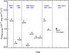 |
Fig. 1 Historical X-ray (0.5–2.0 keV) fluxes of1H 0419–577. Each symbol indicates a flux measurement, as obtained at the labeled date. |
XMM-Newton datasets log.
2. 1H 0419–577: a variable Seyfert galaxy
The Seyfert 1.5 (Véron-Cetty & Véron 2006) galaxy1H 0419–577 is a radio quiet quasar located at redshift z = 0.104. The estimated mass for the SMBH harbored in its nucleus is ~3.8 × 10⁸ M⊙ (O’Neill et al. 2005). The source has been targeted by all the major X-ray observatories, and, in Fig. 1 we plot the historical fluxes in the 0.5–2.0 keV band. As noticed for the first time in Guainazzi et al. (1998),1H 0419–577undergoes frequent transitions between low and high flux states. While the bulk of the flux variation occurs in the soft X-ray, the spectral slope flattens out drastically in the hard (2–10 keV) X-ray band (down to Γ = 1.0 in the lowest state, Page et al. 2012; Pounds et al. 2004a). Due to this peculiar behavior in the X-rays,1H 0419–577is challenging for any interpretation, and for this reason, it has been subject of discussion over the past years.
According to Page et al. (2002), the cooling of the plasma temperature in the hot corona may produce the observed flux/spectral transition. Afterwards, Pounds et al. (2004a,b) carried on a systematic study of the spectral variability in this source, using five ~15 ks long observations, which had been taken during one year with a time spacing of ~3 months. These authors concluded that the spectral variability is dominated by an emerging/disappearing steep power-law component, which is, in turn, modified by a slightly ionized variable absorber. The fitted absorber becomes more ionized and less opaque as the continuum flux increases, supporting the idea that a fraction of the soft X-ray emission may be due to re-emission of the absorbed continuum in an extended region of photoionized gas. An alternative explanation of the same XMM-Newton datasets was, however, readily proposed in the framework of blurred reflection model (Fabian et al. 2005, hereafter F05). This model prescribes that AGN spectral variability is due to the degree of light-bending, as the primary power-law emitting spot moves in a region of stronger gravity. Low flat states, such as the ones observed in1H 0419–577, are extreme reflection-dominated cases occurring when the primary emission is almost completely focused down to the disk and do not reach the observer. The broader spectral coverage provided by two subsequent Suzaku observations of1H 0419–577did not break this models degeneracy. The variable excess observed above ~15 keV can be either explained by reflection (Walton et al. 2010; Pal & Dewangan 2013) or by reprocessing of the primary emission in a partially covering Compton-thick, screen of gas (Turner et al. 2009). The high ionization parameter suggests that this absorber may be part of a clumpy disk wind located within the broad line region (BLR).
In this paper, we present the longest exposure EPIC-pn dataset of 1H 0419-577 that has been obtained so far. The XMM-Newton observation was taken simultaneously to a HST-COS observation in the UV (Edmonds et al. 2011) and caught the source in an intermediate flux state (Fig. 1). In the Reflection Grating Spectrometer (RGS) spectrum of this dataset (already presented in Di Gesu et al. 2013, hereafter Paper I) we detected a lowly ionized absorbing gas (also observed in Suzaku, Winter et al. 2012). We found that the X-ray and the UV absorbing gas (Edmonds et al. 2011) are consistent to be one and the same. The low-gas density estimated in the UV and the low ionization parameter that we measured in the X-ray imply a galactic scale location for the absorbing gas (d ~ 4 kpc). In this respect, the warm absorber in1H 0419–577represents a unique case, being the first X-ray absorber ever detected so far away from the nucleus. The absorbing gas does not have an emission counterpart since more highly ionized lines which are produced by elements such as O vii, O viii, and Ne ix, are the most prominent emission features in the X-ray spectrum. The photoionization modeling of the X-ray and UV narrow emission lines confirmed that they are produced by a more highly ionized gas phase which is located closer (~1 pc) to the nucleus.
In the present analysis, we exploit the simultaneous UV and optical (thanks to the XMM-Newton Optical Monitor) coverage to model the X-ray spectrum in a broadband context using Comptonization. The paper is organized as follows: in Sect. 3, we explain the data reduction procedure; in Sect. 4, we present the spectral analysis of our dataset; in Sect. 5, we apply our best fit model to the past XMM-Newton datasets with the aim of explaining the historical spectral variability; finally we discuss our results in Sects. 6 and 7 we outline our conclusions. The cosmological parameters used are: H0 = 70 km s-1 Mpc-1, Ωm = 0.3 and ΩΛ = 0.7. The C statistic (Cash 1979) is used throughout the paper, and errors are quoted at 90% confidence levels (ΔC = 2.7). In all the spectral models presented in the following, we consider the Galactic hydrogen column density from Kalberla et al. (2005,NH = 1.26 × 1020 cm-2.
3. Observations and data preparation
The source was observed in May 2010 with XMM-Newton for ~167 ks. The observing time was split into two observations (Obs. ID 0604720301 and 0604720401, respectively) which were performed in two consecutive satellite orbits. For the present analysis, we used the EPIC-pn (Strüder et al. 2001) and the Optical Monitor (OM, Mason et al. 2001) data. Besides the HST-COS observation simultaneous to our XMM-Newton observation in the UV the source has been observed twice with the Far Ultraviolet Space Explorer (FUSE), respectively, in 2003 and 2006. In this analysis we used the FUSE flux measurements reported in the literature (Dunn et al. 2008; Wakker & Savage 2009). Finally, we retrieved all the available archival datasets from the XMM-Newton archive and we used them to study the source variability.
3.1. X-ray data
We processed the present datasets and all the archival Observation Data Files (ODF) with the XMM-Newton Science Analysis System (SAS) version 10.0, and with the HEAsoft FTOOLS version 6.12. We refer the reader to Paper I for a detailed description of the data reduction.
For the present datasets, we extracted the EPIC-pn spectra from both 0604720301 and 0604720401 observation. We checked the stability of the spectrum in the two observations, and we found no flux variability larger than ~7%. Therefore, we summed the two spectra into a single combined spectrum with a net exposure time of ~97 ks after the background filtering. We used the FTOOLS mathpha and addarf to combine, respectively, the spectra and the Ancillary Response Files (ARF).
We reduced all the archival datasets following the same standard procedure described in Paper I, and we discarded the datasets with ID 0148000301 and 0148000701, because they show a high contamination by background flares. Hence, we created the EPIC-pn spectra and spectral response matrices for all the good datasets.
We fitted all the X-ray spectra in the 0.3–10 keV band and we rebinned them to have at least 20 counts in each spectral bin, although this is not strictly necessary when using the C statistics. In Table 1, we provide the most relevant information of each XMM-Newton observation, and we label them with numbers, following a chronological order.
3.2. Optical and UV data
As also described in Paper I, in our XMM-Newton observation OM data were collected in four broad-band filters: B,UVW1,UVM2, and UVW2. In the present analysis, we used the OM filters count-rates for the purpose of spectral fitting. Therefore, we also retrieved the spectral response matrices correspondent to each filter from the ESA website1. We corrected the flux in the B filter to account for the host galaxy starlight contribution. For this, we used the same correction factor (56%) estimated in M11 for the stellar bulge of Mrk 509. Since Mrk 509 hosts a BH with a mass similar to the one in1H 0419–577, the stellar mass of the bulge should also be similar in this two galaxies (e.g., Merritt & Ferrarese 2001).
In Paper I, we derived a value for the UV flux of the source at 1500 Å from the continuum of the HST-COS spectrum. Moreover, two other UV fluxes measured with FUSE are reported in the literature, at 1031 Å (Wakker & Savage 2009) and 1110 Å (Dunn et al. 2008), respectively. When the overlapping wavelength region between COS (2010 observation) and FUSE (2003 and 2009 observations) is considered, the level of the UV continuum of the source is the same (see Wakker & Savage 2009; Edmonds et al. 2011). Therefore, we could safely fit the FUSE fluxes with the COS, OM, and the EPIC-pn data that were simultaneously taken in 2010. For this purpose, we converted the UV fluxes back to count rates. We used the HST-COS sensitivity curve and the FUSE effective area (see also M11) for this. We outline all the UV and optical continuum values for1H 0419–577in Table 2.
To check for a possible variability of the source in the optical-UV, we also obtained the OM fluxes from the archival XMM-Newton observations. For all the archival datasets, except Obs. 1, OM data were available in the U,B,V,UVW1, and UVW2 filters.
OM, FUSE, and HST/COS continuum values for 1H 0419−577.
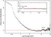 |
Fig. 2 Main panel: model residuals to a power law model in the 0.3–10.0 keV band. A prominent soft excess in the ~0.3−2.0 keV band and a shallow excess at the rest frame energy of theFe Kαtransition are seen. Inset: model residuals to the broadband phenomenological model in 0.3–2.0 keV band. An arc-shaped feature at the rest frame energy of the O vii−O viii transitions is seen. |
4. Spectral modeling
4.1. A phenomenological model
We started with a pure phenomenological modeling of the present EPIC-pn spectrum using SPEX (Kaastra et al. 1996) version 2.04.00. We first attempted to fit the spectrum in the 2.0–10.0 keV energy region with a canonical simple power law (Γ ~ 1.6). The broadband residuals (Fig. 2) show large deviations from this simple model. Besides a prominent soft excess in the 0.3–2.0 keV band, the model does not account for a broad trough between 2.0 and 4.0 keV. To phenomenologically account for this nontrivial spectral shape, a combination of four different spectral slopes would be required all over the 0.3–10.0 keV band. Nonetheless, a prominent peak in the model residuals (Fig. 2) at ~0.5 keV is still unaccounted. We identified this feature as due to the blend of the O vii-O viii lines that we detected in the simultaneous RGS spectrum (Paper I). Furthermore, a shallow excess is seen at ~5.5 keV. Fitting this feature with a delta-shaped emission line which is centered at the nominal rest frame energy of theFe Kαline-transition, does not leave any prominent structure in the residuals. If the line width is left free to vary, the fitted line-width (σ = 300 ± 200 eV) is well consistent with what was previously reported for this source (Turner et al. 2009; Pounds et al. 2004a,b). We also attempted to decompose theFe Kαin a combination of a broad plus a narrow component, but this exercise did not lead to a conclusive result. Despite the good data quality of the present dataset, the line-width of the broad component and the normalization of the narrow component cannot be constrained simultaneously.
In conclusion, the long exposure time of the present EPIC-pn spectrum unveiled a complex continuum spectral structure, which calls for more physically motivated modeling to be fully understood.
4.2. Reflection fitting
At first, we tested a disk reflection scenario for the present spectrum. As noticed in Sect. 1, this model has already been successfully applied to Obs. 1–5 (F05). Besides the main power law continuum, the second relevant spectral component in this model is a relativistically smeared reflected power law, which is thought to be produced in an ionized accretion disk.
We fitted the spectrum with Xspec (Arnaud 1996) version 12.0, and we used PHABS to account for the Galactic hydrogen column density along the line of sight. We used REFLIONX (Ross & Fabian 2005) to model the reflected component, and we left the ionization parameter of the reflector free to vary. Hence, we accounted for the relativistic effects from an accretion disk that surrounds a rotating black hole (Laor 1991) with KDBLUR2. The free parameters in this component are the disk inclination and inner radius, along with the slopes and the break radius of the broken power law shaped emissivity profile. We kept the outer radius frozen to the default value of 400 gravitational radii (Rg), and we set the iron abundance to the solar value (Anders & Grevesse 1989). We extended the model calculation to a larger energy range (0.1–40 keV) to avoid spurious effects due to a truncated convolution. We also attempted to fit the spectrum with a composite disk model (see F05), by splitting the disk in two regions with different ionization parameters to mimic a more realistic scenario where the disk ionization varies with the radius. However, with a simple reflection model we already obtained a statistically good fit, which was not strikingly improved (ΔC = 29) by using a more complex composite disk model. We list the best fit parameters of the reflection fitting in Table 3. Overall, our result agrees with the main predictions of the physical picture proposed in F05. The black hole hosted in1H 0419–577may be rapidly spinning, as suggested by the proximity of the fitted disk inner radius to the value of the innermost stable orbit of a maximally rotating Kerr black hole. The steep emissivity profile of the disk indicates that it is illuminated mostly in its inner part, as it is expected if the primary continuum is emitted very close to the BH. In this framework, the historical source variability is due to the variable light bending, which may produce a negative trend of the reflection fraction with the power law flux. Our results are consistent with the general trend noticed in F05 (Fig. 3).
Best fit parameters for the reflection fitting.
4.3. Broadband spectral modeling
The AGN emission can be also produced by thermal Comptonization (see Sect. 1). This model has the advantage of explaining AGN emission in a consistent way over the entire optical, UV, and X-ray energy range (e.g., Mrk 509, M11, P13). Indeed, the disk blackbody temperature that can be constrained from a fit of the optical/UV data serves as input for the Comptonized components that produce the X-ray continuum. The model includes both a warm (hereafter labeled as “wc”) and a hot Comptonizing corona (hereafter labeled as “hc”) to cover the entire X-ray bandpass. Given the simultaneous X-ray, UV, and optical coverage available in the present case, it is worthwhile testing also this scenario.
We fitted the EPIC-pn spectrum of1H 0419–577with the COS, FUSE, and OM count-rates with SPEX. We left the normalization of each instrument relative to the EPIC-pn as a free parameter to account for the diverse collecting area of different detectors. In the fit, we both accounted for the Galactic absorption and for the local warm absorber that we detected in Paper I. For the former, we used the SPEX collisionally-ionized plasma model (HOT), setting a low temperature (0.5 eV) to mimic a neutral gas. The cosmological redshift (z = 0.104) was also considered in the fit. The final multicomponent model is plotted in Fig. 4.
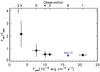 |
Fig. 3 Reflection fraction as a function of the power law flux with errors. The reflection fraction is given by the ratio between the 0.5–10.0 keV fluxes of the reflected component to the primary power law. The value for the present dataset is labeled, while all the other data points, including a lower limit indicated by an arrow, are taken from F05. The observation numbers for each data point are labeled on the upper axis (see Table 1). Note that the data point labeled with an “X” has not been used in the present analysis (see Sect. 3.1). |
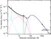 |
Fig. 4 Best fit Comptonization model for1H 0419–577. Solid line: total model. Crosses: fluxed EPIC-pn spectrum (rebinned for clarity), OM, COS, and FUSE data points with errors. Long-dashed line: disk blackbody component. Dotted line: warm Comptonized component. Dashed line: hot Comptonized component. Dash-dotted line: Gaussian O vii (triplet) emission line. Triple-dot-dashed line: cold reflection component, accounting for theFe Kαemission lines. |
We used the disk blackbody model (DBB) in SPEX to model the optical-UV emission of1H
0419–577. This model is based on a geometrically thin, optically thick, Shakura-Sunyaev
accretion disk (Shakura 1973). The DBB spectral
shape results from the weighed sum of the different blackbody spectra emitted by annuli of
the disk located at different radii. The free parameters are the maximum temperature in
the disk (Tmax) and the normalization
 , where
Rin is the inner radius of the disk and
i is the
disk inclination. Instead, we kept the ratio between the outer and the inner radius of the
disk frozen to the default value of 103. The best-fit parameters of the disk blackbody (Fig.
4, long-dashed line) are: Tmax = 56 ± 6 eV and A = (1.2 ± 0.6) × 1026 cm2.
The fitted intercalibration factors between OM, COS, FUSE, and EPIC-pn with errors are
reported in Table 2. The effect of these
intercalibration corrections is within the errors of the disk blackbody parameters given
above.
, where
Rin is the inner radius of the disk and
i is the
disk inclination. Instead, we kept the ratio between the outer and the inner radius of the
disk frozen to the default value of 103. The best-fit parameters of the disk blackbody (Fig.
4, long-dashed line) are: Tmax = 56 ± 6 eV and A = (1.2 ± 0.6) × 1026 cm2.
The fitted intercalibration factors between OM, COS, FUSE, and EPIC-pn with errors are
reported in Table 2. The effect of these
intercalibration corrections is within the errors of the disk blackbody parameters given
above.
We used the COMT model in SPEX, which is based on the Comptonization model of Titarchuk (1994) to model the X-ray continuum. The seed photons in this model have a Wien-law spectrum with temperature T0. In the fit, we coupled T0 to the disk temperature Tmax. The other free parameters are the electron temperature T and the optical depth τ of the Comptonizing plasma. A combination of two Comptonizing components fits the entire EPIC-pn spectrum. The warm corona (Twc ~ 0.7 keV) is optically thick (τwc ~ 7) and produces the softer part of the X-ray continuum below ~2.0 keV (Fig. 4, dotted line). On the other hand, the hot corona (Thc ~ 160 keV) is optically thin (τhc ~ 0.5) and accounts for the X-ray emission above ~2 keV (Fig. 4, dashed line).
Hence, we identified the remaining features in the model residuals as due to the O vii–O viii (Fig. 4, dash-dotted line) andFe Kαemission lines (Fig. 4, triple-dot-dashed line). We added a broadened Gaussian line to the fit with the line-centroid and the line-width frozen to the values that we obtained in the RGS fit (Paper I) to account for the O vii emission. The fitted line luminosity is consistent with what is reported in Paper I. The shallower O viii line that was present in the RGS spectrum is undetected in the EPIC data. In a Comptonization framework, a possible origin for theFe Kαemission is reflection from a cold, distant matter (e.g., from the torus). We have shown in Sect. 4.1 that theFe Kαline in1H 0419–577might also be broad. Detailed study of the properties of theFe Kαemission line produced in cold matter show that the line may appear broadened in some conditions because of the blend between the main line core and the so-called “Compton shoulder” (see Yaqoob & Murphy 2011). The predicted apparent line broadening is consistent with what we have obtained in Sect. 4.1 from a phenomenological fit of a possible line-width. We added a REFL component to the fit to test this possibility. We considered an incident power law with a cutoff energy of 150 keV with the same slope and normalization that we derived from the phenomenological fit (Sect. 4.1). We set a null ionization parameter and a low gas temperature (T ~ 1 eV) to mimic a neutral reflector, and, to adapt the model to the data, we left only the scaling factor2 (s) free to vary. A reflected component with s = 0.3 ± 0.1 satisfactorily fits theFe Kαline and slightly adjusts the underlying continuum (ΔC = −7).
We list the luminosities of all the model components in Table 4, while the parameters and errors of the Comptonized components are outlined in Table 5.
Luminosities of the broadband model components.
Best fit parameters and errors, for the absorbed Comptonization model.
5. Historical spectral variability
5.1. Baseline model
In Fig. 5, we plot the historical X-ray, optical, and UV fluxes of1H 0419–577from the archival XMM-Newton observations and from the present dataset. The optical-UV flux of the source has been stable throughout the ~8 years during which OM observations are available (Obs 2–6). Nevertheless, as already pointed out in Sect. 2 the source has been observed by XMM-Newton in a variety of flux states in the soft X-rays (see Fig. 5), ranging from the deep flux minimum of September 2002 (Obs. 2) to the highest state of December 2000 (Obs. 1). We used the Comptonization model that successfully fitted the present dataset as a baseline model for the fit of the past XMM-Newton observations. Because the maximum observed variability in the optical-UV (~20%) is within the errors in the disk blackbody parameters that we derived in the broadband fitting (Sect. 4.3), we assumed the same seed photons temperature of the present dataset in the baseline model.
In Fig. 6, we plot the historical fluxes of theFe Kαemission line that were measured from a phenomenological fit of the archival and present XMM-Newton datasets in the 2.0–10.0 keV band. Although the line is not well constrained in any of the archival datasets, its flux is, however consistent to have been stable in the ~10 year-long period covered by XMM-Newton observations. Therefore, the cold reflection continuum associated to theFe Kαline should have remained constant. Since we are mainly interested in studying the source variability in the soft X-ray band, we included just a delta function to account for theFe Kαemission line in the baseline model. Indeed, the addition of a cold reflection continuum is not critical for the resulting parameters. Finally, we included unresolved O vii-f and O viii-Ly αemission lines in the baseline model. Previous analysis of the RGS spectrum (Pounds et al. 2004b) has shown that O vii and O viii lines were present in Obs 2–5. The baseline model provides a formally acceptable fit for all the datasets except Obs. 2, namely the lowest flux state.
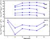 |
Fig. 5 Upper panel: variability of the optical and UV fluxes in the OM broadband filters for the archival and present XMM-Newton datasets. Lower panel: variability of the soft (0.5–2.0 keV) and hard (2.0−10.0 keV) X-ray fluxes. |
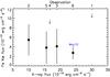 |
Fig. 6 Historical and present observed fluxes of theFe Kαemission line with errors as a function of the source flux in the 0.5–10.0 keV band. The arrows represent upper limits for the line flux. The value for the present dataset is labeled, and the observation numbers for each data point (see Table 1) are labeled as well on the upper axis. |
5.2. Low flux state
We show a comparison between the low-state spectrum and the present dataset in Fig. 7. At a first glance, the spectrum appears much flatter in the ~1.0–2.0 keV band and displays a peak at ~0.5 keV resembling the shape of an emission line. Indeed, this feature is well modeled by the O vii−O viii emission lines that are present in the baseline model. The fitted line fluxes (FO vii = (16 ± 8) × 10-5 photons s-1 cm-2and FO viii = (8 ± 4) × 10-5 photons s-1 cm-2) are consistent with what previously reported for the RGS spectrum of this dataset (Pounds et al. 2004a). The residuals to the baseline model display a deep trough, approximately in the same energy region where the spectrum flattens out with respect to the present dataset. We added to the fit a neutral absorber located at the redshift of the source, modeled by a cold (T = 0.5 eV) collisionally-ionized plasma (HOT model in SPEX) to attempt adapting the baseline model to the low-state spectrum. By letting all the Comptonized emission being absorbed by a partially covering (~60%), thick ( NH~ 5 × 1022 cm-2) cold gas, we achieved a statistically good (C/d.o.f. = 163/152) fit to the data, accounting for all the features left in the residuals by an unabsorbed model.
5.3. Partial covering of the baseline model
Prompted by the results of the low state fit, we checked if the addition of a cold absorber could also improve the fit of the other datasets. We outline the results of this exercise for all the archival datasets in Table 5. An additional partially-covering absorbing component with a similar covering factor (~50%) but a lower column density provides a significant improvement of the fit for Obs. 3–5. In contrast, no absorbing component is statistically required in the fit of Obs. 1 and and 6, namely the two highest flux states. For these datasets, we set an upper limit to the absorbing column density by keeping the covering factor fixed to ~0.5. In Fig. 8, we plot the parameters of the absorber as a function of the source flux. The absorbing column density shows a negative trend with the flux, while the covering fraction is consistent to be constant. The variable absorbing component does not, however, account for all the source variability. As we show in Fig. 9, we still observe an intrinsic variability in both the two Comptonized components after removing the effect of the variable absorption.
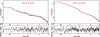 |
Fig. 7 EPIC-pn spectrum of1H 0419–577in the low flux state (Obs. 2, left panel) and in the present intermediate flux state (Obs. 6, right panel). The best fit Comptonization model is displayed as a solid line. Model residuals, in terms of σ, are also shown. We rebinned the spectra for clarity purposes. Note that error bars are as large as the thickness of the model line for the present dataset. |
We also tested a different scenario where the absorber is constant in opacity and its variability is driven only by a variable covering fraction. At this purpose, we attempted to fit Obs. 4 and 5 keeping the absorber column density frozen to the value observed in the low-flux state and letting only the covering factor free to vary. In both cases, we had to release the parameters of the underlying continuum to achieve an acceptable fit. In detail we obtained a covering factor of ~4% for Obs. 4 but the model residuals are important between 2 and 5 keV. In Obs. 5, the fit erases the absorber pushing the covering factor to a much lower value (~0.03%). In both cases, the fit is statistically worse (C/d.o.f = 216/152 and 152/139 respectively) than what is reported in Table 5. Thus, we rejected this possibility, and we concluded that the absorber model outlined in Table 5 better fits the data.
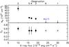 |
Fig. 8 Variability of the local neutral absorber in1H 0419–577. The gas column density (upper panel) and and covering factor (lower panel) with errors are plotted against the observed source flux in the 0.5–10.0 keV band. Arrows represent upper limits for the column density. Crosses represent fixed values for the covering factor. The values for the present dataset are labeled, and the observation numbers for each data point (see Table 1) are labeled as well on the upper axis. |
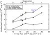 |
Fig. 9 Variability of the intrinsic 0.5–10.0 keV luminosity in1H 0419–577. The unabsorbed luminosities of the hot and the warm Comptonized component, along with the total intrinsic luminosities are plotted against the observed source flux in the 0.5–10.0 keV band. The symbols are outlined in the legend. Error bars, when larger than the size of the plotted symbols, are also shown. The values for the present dataset are labeled and the observation numbers for each data point (see Table 1) are labeled as well on the upper axis. |
6. Discussion
6.1. X-ray spectrum of1H 0419–577
The long exposure XMM-Newton observation of1H 0419–577that we presented in this paper provided a high-quality X-ray spectrum which is suitable for testing physically motivated models against real data. Exploiting the simultaneous coverage in the optical/UV that was provided in the present case by the OM and by HST-COS, we successfully represented the broadband spectrum of1H 0419–577using Comptonization. The emerging physical picture provided that the optical-UV disk photons (T ~ 56 eV) are both Comptonized by an optically thick (τwc ~ 7) warm medium (Twc ~ 0.7 eV) and by an optically thinner (τhc ~ 0.5) and hotter (Thc ~ 160 keV) plasma to produce the entire X-ray spectrum.
A similar interpretation has been recently proposed for the broadband simultaneous spectrum of Mrk 509 (M11, P13) and also for a sample of unobscured type 1 AGN (Jin et al. 2012). A reasonable configuration for these two media in the inner region of AGN is possible. Two different Comptonizing coronae may be present. The geometrically compact hot corona may be associated with the inner part of the accretion flow, while the warm corona may be a flat upper layer of the accretion disk (P13). Alternatively, according to a model proposed in Done et al. (2012), the warm Comptonization may take place in the accretion disk itself below a critical radius after which the radiation cannot thermalize anymore. It is in principle also possible that the seed photons are provided to the hot corona by the soft excess component (e.g., PKS 0558-504, Gliozzi et al. 2013). We note that the broadband spectrum of1H 0419–577is consistent with a “nested-Comptonization” scenario provided a slightly thicker warm Comptonized component (τ ~ 11). Finally, we suggest that theFe Kαemission line in1H 0419–577is produced by reflection in a cold thick torus. The long-term flux stability of the line that we note in Fig. 6 supports this interpretation.
Tombesi et al. (2010) reported the detection of an ultra fast outflow (UFO) in1H 0419–577. According to these authors, the signature of the UFO is a blushifted Fe xxvi-Ly αabsorption line located at a restframe energy of ~7.23 keV which is possibly accompanied by a Fe xxv feature at ~8.4 keV. Despite the high signal-to-noise ratio none of these features is evident in the present spectrum. We estimated upper limits for the equivalent width (EW) of the main UFO absorption lines, assuming the same outflow velocity given in Tombesi et al. (2010, v ~ 11 100 km s-1. The deepest UFO that is consistent with our dataset is much shallower than what previously reported, because we found EW ≲ 12 eV and EW ≲ 9 eV for the Fe xxvi-Ly αand Fe xxv-Heα transition, respectively.
6.2. Historical spectral variability of1H 0419–577
The Seyfert galaxy1H 0419–577is well known for showing a remarkable flux variability in the X-rays that is accompanied by a dramatical flattening of the spectral slope as the source flux decreases. Nonetheless, the optical/UV fluxes that were observed in diverse X-ray flux states are rather stable. In Sect. 5, we showed that a Comptonization model can explain the historical spectral variability of1H 0419–577, provides an intrinsic variability of the two Comptonized components, and a partially-covering, cold absorption variable in opacity.
The intrinsic variability of the X-ray Comptonized continuum is easy to justify. Indeed, Monte Carlo computations of X-ray spectra from a disk-corona system show that coronae may be intrinsically variable even when given an optical depth and a electron temperature. Without requiring variations in the accretion rate that would be inconsistent with the stability of the optical/UV flux, a substantial variability may be induced, for instance, by geometrical variations (e.g., Sobolewska et al. 2004) or by variations in the bulk velocity of the coronal plasma (e.g., in a non static corona, Malzac et al. 2001).
However, apart from the smaller intrinsic variation, the variable cold absorption causes the bulk of the observed spectral variability. In this respect,1H 0419–577is not a unique case. So far, cold absorbers variable on a broad range of timescales (few hours−few years) have been detected in a handful of cases, (e.g., NGC 1365, NGC 4388, and NGC 7582, Risaliti et al. 2005; Elvis et al. 2004; Piconcelli et al. 2007) including some optically unobscured, standard type 1 objects (e.g., NGC 4151, 1H0557-385, Mrk 6 Puccetti et al. 2007; Longinotti et al. 2009; Immler et al. 2003) and narrow line Seyfert 1 (e.g., SWIFT J2127.4+5654 Sanfrutos et al. 2013). In most of these cases, discrete clouds of cold gas with densities and sizes typical of the BLR clouds may cause the variable absorption. The estimated location of these clouds is within the “dust sublimation radius”, which nominally separates the BLR and the obscuring torus. This indicates that the distribution of absorbing material in AGN may be more complex than the axisymmetric torus that is prescribed by the standard unified model (see Bianchi et al. 2012, and references therein).
The variation of the cold absorber in1H 0419–577is driven by a decreasing opacity, which
seems to show a trend with the increasing flux (Fig. 8, upper panel). In in the two highest flux spectra, the absorbing column
density is consistent to have been at least a factor ~40 thinner than in the lowest flux
spectrum. At the same time, the absorber covering factor remained constant
(~0.5) within the given
errors. A simple explanation for this behavior is that the neutral column density became
ionized in the highest flux dataset because it responded to the enhanced X-ray ionizing
continuum. An inspection of the archival RGS spectra (Pounds et al. 2004a,b) may provide
additional support to this hypothesis. The broad emission features from O vii and
O viii that we detected in the RGS spectrum of the present dataset (Paper I)
are also present in all the past RGS spectra. We note, however, that in the present
dataset, the luminosity of both these lines is lower than what was observed, for instance,
in the lowest flux state (e.g., by a factor ~2 and ~5,
respectively) Moreover, we clearly detected a broad line from a more highly ionized
species (Ne ix, see Paper I), which is undetected in all the archival RGS
spectra. This may be a qualitative indication of a more highly ionized gas in the BLR
during the higher flux state. The enhanced flux may have increased the ionization of the
gas, causing the enhancement of the Ne ix and the decrease of the
O vii-O viii. The difference in unabsorbed continuum luminosities that
we observed, for instance, between the lowest flux state of September 2002 and the
following observation of March 2003 (ΔL ~ 3 × 1044 erg s-1, see Fig. 9) may indeed ionize a cloud of neutral hydrogen with typical BLR
density in the observed timescale (Δt ≲ 7 months). Assuming that the absorber is a
cloud of pure hydrogen that does not change in volume as a consequence of the ionization,
then the fraction of hydrogen that became completely ionized in March 2003 is as follows:
 (1)If the cloud is
illuminated by ΔL the conservation of energy, assuming spherical
symmetry implies that:
(1)If the cloud is
illuminated by ΔL the conservation of energy, assuming spherical
symmetry implies that:  (2)where
Cv is the absorber
covering factor, d is the absorber distance, UH = 13.6 eV is
the ionization threshold of hydrogen, nH is the absorber density, and
f = 10-2 is the volume filling factor of
the broad line region (Osterbrock 1989). Taking the
dust sublimation radius3 (RDUST ~ 0.6 pc)
as an upper limit for the absorber distance from Eq. (2) follows that
(2)where
Cv is the absorber
covering factor, d is the absorber distance, UH = 13.6 eV is
the ionization threshold of hydrogen, nH is the absorber density, and
f = 10-2 is the volume filling factor of
the broad line region (Osterbrock 1989). Taking the
dust sublimation radius3 (RDUST ~ 0.6 pc)
as an upper limit for the absorber distance from Eq. (2) follows that  (3)This lower limit
is well consistent with the typical range of densities of the BLR clouds (108−1012 cm-3, Baldwin et al. 1995).
(3)This lower limit
is well consistent with the typical range of densities of the BLR clouds (108−1012 cm-3, Baldwin et al. 1995).
We also note that this scenario resulted in a statistically better fit of the data than a model mimicking a single cloud with a constant opacity crossing the line of sight (see Sect. 5.3). Indeed, the time interval of a few months separating the XMM-Newton observations of1H 0419–577is inconsistent with the expected duration of an occultation event due to a single BLR cloud. For instance the occultation observed in NGC 1365 (in April 2006, see Risaliti et al. 2007) lasted ~4 days. A similar eclipse, lasting only 90 ks, has been observed in SWIFT J2127.4+5654 (Sanfrutos et al. 2013).
In the scenario we are proposing for1H 0419–577, when the continuum source is found in a low flux state, the surrounding gas is on average less ionized. We suggest, therefore, that in these conditions the number of neutral clouds along the line of sight may be larger, making obscuration events more probable.
We finally remark that a simple argument can explain the stability of the optical/UV continuum in1H 0419–577 in this framework. The optical/UV continuum source is 10 times larger in radius than the X-ray source (see e.g., Elvis 2012). Therefore, a covering on the order of ~50% of the X-ray source implies a negligible covering of the ~0.5% for the optical/UV source.
6.3. Geometry of AGN
We can put significant constraints on the geometry of1H 0419–577from the fitted
parameters of the disk blackbody (Sect. 4.3). The
fitted disk blackbody normalization A is linked to the disk inclination angle
i.
Analytically, 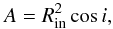 (4)where Rin is the inner
radius of the disk. The disk inner radius may be set by the radius of the innermost stable
circular orbit (RISCO), which is allowed in the
space-time metric produced by the black hole mass (M ~ 3.8 × 10⁸M⊙in this case,
O’Neill et al. 2005) and by its spin. The two
extreme cases are a maximally rotating black hole and a non-rotating Schwarzschild black
hole (see Bambi 2012). Therefore, according to this
general prescription, Rin may only vary in the range:
(4)where Rin is the inner
radius of the disk. The disk inner radius may be set by the radius of the innermost stable
circular orbit (RISCO), which is allowed in the
space-time metric produced by the black hole mass (M ~ 3.8 × 10⁸M⊙in this case,
O’Neill et al. 2005) and by its spin. The two
extreme cases are a maximally rotating black hole and a non-rotating Schwarzschild black
hole (see Bambi 2012). Therefore, according to this
general prescription, Rin may only vary in the range:
![\begin{equation} R_{\rm in}\sim R_{\rm ISCO}=[1{-}6] \,R_{\rm g}, \label{risco} \end{equation}](/articles/aa/full_html/2014/03/aa22916-13/aa22916-13-eq196.png) (5)where Rg = 2GM/c2
is the gravitational radius, G is the gravitational constant, and c is the speed of light.
Combining Eqs. (4) and (5), we obtain:
(5)where Rg = 2GM/c2
is the gravitational radius, G is the gravitational constant, and c is the speed of light.
Combining Eqs. (4) and (5), we obtain:
![\begin{equation} i=[70^{\circ}{-}89^{\circ}]. \end{equation}](/articles/aa/full_html/2014/03/aa22916-13/aa22916-13-eq200.png) (6)To set a more robust
lower limit for the disk inclination angle, we additionally considered the error of the
disk normalization (Sect. 4.3) and of the black hole
mass (~0.5 dex, see O’Neill et al. 2005, and references therein) in the
calculation. With these tighter constraints:
(6)To set a more robust
lower limit for the disk inclination angle, we additionally considered the error of the
disk normalization (Sect. 4.3) and of the black hole
mass (~0.5 dex, see O’Neill et al. 2005, and references therein) in the
calculation. With these tighter constraints:
 (7)These inclination
values are well consistent with the intermediate spectral classification of1H 0419–577as
Seyfert 1.5. It is therefore possible that our viewing direction toward1H 0419–577is
grazing the so-called “obscuring torus” that is prescribed by the standard unified model
(Antonucci 1993). In this framework, the inner
part of the torus may be responsible for the X-ray obscuration.
(7)These inclination
values are well consistent with the intermediate spectral classification of1H 0419–577as
Seyfert 1.5. It is therefore possible that our viewing direction toward1H 0419–577is
grazing the so-called “obscuring torus” that is prescribed by the standard unified model
(Antonucci 1993). In this framework, the inner
part of the torus may be responsible for the X-ray obscuration.
The structure of the obscuring medium in AGN may be more complex than the classical donut torus paradigm. Indeed, this model faces difficulties in explaining several theoretical and observational issues, including, for instance, the wide range of X-ray obscuring column densities (see Elvis 2012, and references therein). A clumpy torus (Nenkova et al. 2008) may alleviate part of these problems. In the latter case, when the numerical density of clouds along the line of sight is low, even a source viewed from a high inclination angle may appear like a Seyfert 1 (see also Elitzur 2012). Moreover, in this model, the BLR and the torus itself are part of the same medium, decreasing in ionization as the distance from the central source increases. Indeed, it has been proposed (see Nenkova et al. 2008) that the clumpy torus extends inward beyond the dust sublimation point. The innermost torus clouds, being more exposed to the ionizing radiation, are probably dust free and may dominate the X-ray obscuration. Given the high viewing angle derived above,1H 0419–577may possibly fit in this framework.
6.4. A comparison with other models
The model that we presented in this paper explains both the optical/UV/X-ray broadband spectrum and the historical variability of1H 0419–577 in a reasonable geometrical configuration. However, the hard X-ray energy range above 10 keV is not covered by the present spectral analysis. In that range,1H 0419–577displays a “hard-excess” (Turner et al. 2009; Pal & Dewangan 2013; Walton et al. 2010) over a simple power law model, that shows some evidence of variability (a factor ~2, see Turner et al. 2009). The extrapolation to harder energies of our broadband model predicts a flux of ~2.9 × 10⁻¹¹ erg s-1 cm-2in the 10–50 keV band. This flux is higher than the 70 month-averaged flux observed with BAT in the same band (~2.2 × 10⁻¹¹ erg s-1 cm-2, Baumgartner et al. 2013) but well consistent with the latest Suzaku measurement taken only 5 months before our XMM-Newton observations (~2.7 × 10⁻¹¹ erg s-1 cm-2, Pal & Dewangan 2013). Because of this relatively short time interval between the Suzaku and XMM-Newton observation, it is indeed likely that Suzaku caught the source in the same flux condition of our observation (see also Fig. 1). In the context of the Suzaku data analysis (Pal & Dewangan 2013), the authors also attempted to fit a Comptonization model to the May 2010 EPIC-pn spectra. They obtained, however, a poor result mainly because of a prominent excess in the residuals near ~0.5 keV. In the present analysis, thanks to the higher resolution provided by the RGS, we could easily identify that feature as due to the O vii line complex. Apart from this discrepancy, the parameters they obtained for the warm Comptonized component reasonably agree with our result.
On a different occasion (July 2007), Suzaku caught the source in a bright state, similar to what was observed by XMM-Newton in December 2000 (Obs. 1). The hard X-ray curvature that was observed in that case (F15−50 keV ~ 2.6 × 10⁻¹¹ erg s-1) can be fitted using a Compton-thick, highly ionized absorption, covering ~66% of the line of sight. To check if our model could also explain this historical hard X-ray maximum, we compared the hard X-ray flux extrapolated by the fit of Obs. 1 with the one observed by Suzaku. We noted a small disagreement as the flux predicted by our model is by a factor of 1.6 lower than the observed one. Thus, we cannot definitively rule out that a partially-covering ionized absorber was present in the high flux state of July 2007. In the framework proposed in this paper, it may in principle be the ionized counterpart of the cold absorber present in the low flux state.
Besides our interpretation, the light bending model may also explain the variable X-ray spectrum of this source and fits both the XMM-Newton and the Suzaku datasets (F05, Walton et al. 2010; Pal & Dewangan 2013, this paper). We note, however, that a variable absorption is required to fit the data even in this disk-reflection framework. Indeed, a cold absorber showing the same trend noticed here (with a column density dropping fromNH≃ 1021 cm-2 to 0) is present in the F05 model. Additionally, an O vii edge with a variable depth, which mimics an ionized warm absorber, is also included. The latter is somewhat at odds with what we reported in Paper I because the warm absorber in1H 0419–577is too lowly ionized to produce any strong O vii absorption features. Moreover, a short timescale variation of the ionized absorption edges, as required in F05, is difficult to reconcile with the galactic scale location (see Paper I) of the warm absorber in this source. In our analysis, solar abundances are adequate to fit the data. In the light bending model, the metal abundance in the disk is a free parameter, and it has been reported to vary from supersolar in September 2002 (~3.8, F05) to undersolar in January 2010 (~0.5, Pal & Dewangan 2013). This is another issue that is difficult to explain. Finally, we note that a physical interpretation of the source variability that is observed with Suzaku is not possible in the context of the light bending model alone, and additional variability in the disk-corona geometry, possibly caused by a variability in the accretion rate (that would be however inconsistent with the stability of the optical/UV flux noticed here) has to be invoked (Pal & Dewangan 2013).
In conclusion, the Comptonization model proposed here for the present and historical broadband spectrum of1H 0419–577does not rule out other possible interpretations. It has, however, the advantage of explaining all the observational evidences collected in the last ten years over the broadest range of wavelength available without requiring any special ad hoc assumption. A future observation in the entire X-ray band with XMM and NuSTAR would be important to solve the long-standing ambiguity in the interpretation of the spectral variability in this peculiar Seyfert galaxy.
7. Summary and conclusions
We modeled the broadband optical (XMM-OM), UV (HST-COS, FUSE), and X-ray (EPIC-pn) simultaneous spectrum of1H 0419–577taken in May 2010 using Comptonization. The X-ray continuum may be produced by a warm (Twc ~ 0.7 keV, τwc ~ 7) and a hot Comptonizing medium (Thc ~ 160 keV, τ ~ 0.5) which are both fed by the same optical/UV disk photons (Tdbb ~ 56 eV). The hot medium may be a geometrically compact corona located in the innermost region of the disk. The warm medium may be an upper layer of the accretion disk. Reflection from cold distant matter is a possible origin for theFe Kα emission line. Despite the long exposure time of our dataset, we do not find evidence of the ultra fast outflow features that have been reported in the past for this source.
Providing a partially covering (~50%) cold absorber with a variable opacity (NH ~ [1019−1022] cm-2) and a small variability intrinsic to the source, this model can also reproduce the historical spectral variability of1H 0419–577. The opacity of the absorber increases as the continuum flux decreases. We argue that the absorber may have the typical density of the BLR clouds and that it becomes optically thinner in the higher flux states because it gets ionized in response to the enhanced X-ray continuum.
Relativistic light-bending remains an alternative explanation for the spectral variability in this source. We note, however, that a variable elemental abundance and a variable absorption are required in this scenario. The latter is difficult to reconcile with the UV/X-rays absorber that we have determined to be located at a ~kpc scale.
Finally, we suggest that1H 0419–577may be viewed from a high inclination angle which marginally intercepts a possibly clumpy obscuring torus. In this geometry, the X-ray obscuration may be associated with the innermost dust free region of the obscuring torus.
The present spectral analysis in the optical/UV/X-ray represents a substantial step forward in the comprehension of this intriguing Seyfert galaxy. However, further investigations (e.g., with NuSTAR) are needed to understand the true nature of the spectral variability of this source.
We estimated the dust sublimation radius of1H 0419–577using the ionizing luminosity given in Paper I and the formula of Barvainis (1987), assuming T = 1500 K for the dust sublimation temperature and a = 0.05μm for the dust grain size.
Acknowledgments
This work is based on observations with XMM-Newton, an ESA science mission with instruments and contributions directly funded by ESA Member States and the USA (NASA). SRON is supported financially by NWO, the Netherlands Organization for Scientific Research.
References
- Anders, E., & Grevesse, N. 1989, Geochim. Cosmochim. Acta, 53, 197 [Google Scholar]
- Antonucci, R. 1993, ARA&A, 31, 473 [Google Scholar]
- Arnaud, K. A. 1996, in Astronomical Data Analysis Software and Systems V, eds. G. H. Jacoby, & J. Barnes, ASP Conf. Ser., 101, 17 [Google Scholar]
- Arnaud, K. A., Branduardi-Raymont, G., Culhane, J. L., et al. 1985, MNRAS, 217, 105 [NASA ADS] [CrossRef] [Google Scholar]
- Baldwin, J., Ferland, G., Korista, K., & Verner, D. 1995, ApJ, 455, L119 [NASA ADS] [CrossRef] [Google Scholar]
- Ballantyne, D. R., Ross, R. R., & Fabian, A. C. 2001, MNRAS, 327, 10 [NASA ADS] [CrossRef] [Google Scholar]
- Ballantyne, D. R., Vaughan, S., & Fabian, A. C. 2003, MNRAS, 342, 239 [NASA ADS] [CrossRef] [Google Scholar]
- Bambi, C. 2012, Phys. Rev. D, 85, 043001 [CrossRef] [Google Scholar]
- Barvainis, R. 1987, ApJ, 320, 537 [NASA ADS] [CrossRef] [Google Scholar]
- Baumgartner, W. H., Tueller, J., Markwardt, C. B., et al. 2013, ApJS, 207, 19 [NASA ADS] [CrossRef] [EDP Sciences] [Google Scholar]
- Bianchi, S., Maiolino, R., & Risaliti, G. 2012, Adv. Astron., 2012, accepted [arXiv:1201.2119] [Google Scholar]
- Cappi, M., Panessa, F., Bassani, L., et al. 2006, A&A, 446, 459 [NASA ADS] [CrossRef] [EDP Sciences] [Google Scholar]
- Cash, W. 1979, ApJ, 228, 939 [NASA ADS] [CrossRef] [Google Scholar]
- Crummy, J., Fabian, A. C., Gallo, L., & Ross, R. R. 2006, MNRAS, 365, 1067 [NASA ADS] [CrossRef] [Google Scholar]
- Di Gesu, L., Costantini, E., Arav, N., et al. 2013, A&A, 556, A94 (Paper I) [NASA ADS] [CrossRef] [EDP Sciences] [Google Scholar]
- Done, C., Davis, S. W., Jin, C., Blaes, O., & Ward, M. 2012, MNRAS, 420, 1848 [NASA ADS] [CrossRef] [Google Scholar]
- Dunn, J. P., Crenshaw, D. M., Kraemer, S. B., & Trippe, M. L. 2008, AJ, 136, 1201 [NASA ADS] [CrossRef] [Google Scholar]
- Edmonds, D., Borguet, B., Arav, N., et al. 2011, ApJ, 739, 7 [NASA ADS] [CrossRef] [Google Scholar]
- Elitzur, M. 2012, ApJ, 747, L33 [NASA ADS] [CrossRef] [Google Scholar]
- Elvis, M. 2012, J. Phys. Conf. Ser., 372, 012032 [CrossRef] [Google Scholar]
- Elvis, M., Risaliti, G., Nicastro, F., et al. 2004, ApJ, 615, L25 [NASA ADS] [CrossRef] [Google Scholar]
- Fabian, A. C., Miniutti, G., Iwasawa, K., & Ross, R. R. 2005, MNRAS, 361, 795 [Google Scholar]
- Gliozzi, M., Papadakis, I. E., Grupe, D., Brinkmann, W. P., & Räth, C. 2013, MNRAS, 433, 1709 [NASA ADS] [CrossRef] [Google Scholar]
- Guainazzi, M., Comastri, A., Stirpe, G. M., et al. 1998, A&A, 339, 327 [NASA ADS] [Google Scholar]
- Haardt, F., & Maraschi, L. 1991, ApJ, 380, L51 [NASA ADS] [CrossRef] [Google Scholar]
- Immler, S., Brandt, W. N., Vignali, C., et al. 2003, AJ, 126, 153 [NASA ADS] [CrossRef] [Google Scholar]
- Jin, C., Ward, M., Done, C., & Gelbord, J. 2012, MNRAS, 420, 1825 [NASA ADS] [CrossRef] [Google Scholar]
- Kaastra, J. S., Mewe, R., & Nieuwenhuijzen, H. 1996, in UV and X-ray Spectroscopy of Astrophysical and Laboratory Plasmas, eds. K. Yamashita, & T. Watanabe (Tokyo: Universal Academic Press, Inc.), 411 [Google Scholar]
- Kaastra, J. S., Petrucci, P.-O., Cappi, M., et al. 2011, A&A, 534, A36 [NASA ADS] [CrossRef] [EDP Sciences] [Google Scholar]
- Kalberla, P. M. W., Burton, W. B., Hartmann, D., et al. 2005, A&A, 440, 775 [NASA ADS] [CrossRef] [EDP Sciences] [Google Scholar]
- Laor, A. 1991, ApJ, 376, 90 [NASA ADS] [CrossRef] [Google Scholar]
- Longinotti, A. L., Bianchi, S., Ballo, L., de La Calle, I., & Guainazzi, M. 2009, MNRAS, 394, L1 [NASA ADS] [CrossRef] [Google Scholar]
- Magdziarz, P., Blaes, O. M., Zdziarski, A. A., Johnson, W. N., & Smith, D. A. 1998, MNRAS, 301, 179 [NASA ADS] [CrossRef] [Google Scholar]
- Malzac, J., Beloborodov, A. M., & Poutanen, J. 2001, in Gamma 2001: Gamma-Ray Astrophysics, eds. S. Ritz, N. Gehrels, & C. R. Shrader, AIP Conf. Ser., 587, 111 [Google Scholar]
- Mason, K. O., Breeveld, A., Much, R., et al. 2001, A&A, 365, L36 [NASA ADS] [CrossRef] [EDP Sciences] [Google Scholar]
- Mehdipour, M., Branduardi-Raymont, G., Kaastra, J. S., et al. 2011, A&A, 534, A39 [NASA ADS] [CrossRef] [EDP Sciences] [Google Scholar]
- Merritt, D., & Ferrarese, L. 2001, ApJ, 547, 140 [NASA ADS] [CrossRef] [Google Scholar]
- Middleton, M., Done, C., & Gierliński, M. 2007, MNRAS, 381, 1426 [NASA ADS] [CrossRef] [Google Scholar]
- Miller, L., Turner, T. J., & Reeves, J. N. 2008, A&A, 483, 437 [NASA ADS] [CrossRef] [EDP Sciences] [Google Scholar]
- Morgan, C. W., Kochanek, C. S., Dai, X., Morgan, N. D., & Falco, E. E. 2008, ApJ, 689, 755 [NASA ADS] [CrossRef] [Google Scholar]
- Nenkova, M., Sirocky, M. M., Nikutta, R., Ivezić, Ž, & Elitzur, M. 2008, ApJ, 685, 160 [NASA ADS] [CrossRef] [Google Scholar]
- Novikov, I. D., & Thorne, K. S. 1973, in Black Holes (Les Astres Occlus), eds. C. Dewitt, & B. S. Dewitt (New York: Gordon & Breach), 343 [Google Scholar]
- O’Neill, P. M., Nandra, K., Papadakis, I. E., & Turner, T. J. 2005, MNRAS, 358, 1405 [NASA ADS] [CrossRef] [Google Scholar]
- Osterbrock, D. E. 1989, Astrophysics of Gaseous Nebulae and Active Galactic Nuclei, (Mill Valley: University Science Books) [Google Scholar]
- Page, K. L., Pounds, K. A., Reeves, J. N., & O’Brien, P. T. 2002, MNRAS, 330, L1 [NASA ADS] [CrossRef] [Google Scholar]
- Page, M. J., Symeonidis, M., Vieira, J. D., et al. 2012, Nature, 485, 213 [NASA ADS] [CrossRef] [Google Scholar]
- Pal, M., & Dewangan, G. C. 2013, MNRAS, 435, 1287 [NASA ADS] [CrossRef] [Google Scholar]
- Panessa, F., Bassani, L., de Rosa, A., et al. 2008, A&A, 483, 151 [NASA ADS] [CrossRef] [EDP Sciences] [Google Scholar]
- Perola, G. C., Matt, G., Cappi, M., et al. 2002, A&A, 389, 802 [Google Scholar]
- Petrucci, P.-O., Paltani, S., Malzac, J., et al. 2013, A&A, 549, A73 [NASA ADS] [CrossRef] [EDP Sciences] [Google Scholar]
- Piconcelli, E., Jimenez-Bailón, E., Guainazzi, M., et al. 2005, A&A, 432, 15 [NASA ADS] [CrossRef] [EDP Sciences] [Google Scholar]
- Piconcelli, E., Bianchi, S., Guainazzi, M., Fiore, F., & Chiaberge, M. 2007, A&A, 466, 855 [NASA ADS] [CrossRef] [EDP Sciences] [Google Scholar]
- Piro, L., Matt, G., & Ricci, R. 1997, A&AS, 126, 525 [NASA ADS] [CrossRef] [EDP Sciences] [Google Scholar]
- Pounds, K. A., Reeves, J. N., Page, K. L., & O’Brien, P. T. 2004a, ApJ, 605, 670 [NASA ADS] [CrossRef] [Google Scholar]
- Pounds, K. A., Reeves, J. N., Page, K. L., & O’Brien, P. T. 2004b, ApJ, 616, 696 [NASA ADS] [CrossRef] [Google Scholar]
- Puccetti, S., Fiore, F., Risaliti, G., et al. 2007, MNRAS, 377, 607 [NASA ADS] [CrossRef] [Google Scholar]
- Reis, R. C., & Miller, J. M. 2013, ApJ, 769, L7 [Google Scholar]
- Risaliti, G., Elvis, M., Fabbiano, G., Baldi, A., & Zezas, A. 2005, ApJ, 623, L93 [NASA ADS] [CrossRef] [Google Scholar]
- Risaliti, G., Elvis, M., Fabbiano, G., et al. 2007, ApJ, 659, L111 [NASA ADS] [CrossRef] [Google Scholar]
- Rivers, E., Markowitz, A., Duro, R., & Rothschild, R. 2012, ApJ, 759, 63 [NASA ADS] [CrossRef] [Google Scholar]
- Ross, R. R., & Fabian, A. C. 2005, MNRAS, 358, 211 [Google Scholar]
- Sanfrutos, M., Miniutti, G., Agís-González, B., et al. 2013, MNRAS, accepted [arXiv:1309.1092] [Google Scholar]
- Shakura, N. I. 1973, Sov. Astron., 16, 756 [NASA ADS] [Google Scholar]
- Sobolewska, M. A., Siemiginowska, A., & Życki, P. T. 2004, ApJ, 608, 80 [NASA ADS] [CrossRef] [Google Scholar]
- Strüder, L., Briel, U., Dennerl, K., et al. 2001, A&A, 365, L18 [NASA ADS] [CrossRef] [EDP Sciences] [Google Scholar]
- Titarchuk, L. 1994, ApJ, 434, 570 [NASA ADS] [CrossRef] [Google Scholar]
- Tombesi, F., Cappi, M., Reeves, J. N., et al. 2010, A&A, 521, A57 [NASA ADS] [CrossRef] [EDP Sciences] [Google Scholar]
- Turner, T. J., Miller, L., Kraemer, S. B., Reeves, J. N., & Pounds, K. A. 2009, ApJ, 698, 99 [NASA ADS] [CrossRef] [Google Scholar]
- Véron-Cetty, M.-P., & Véron, P. 2006, A&A, 455, 773 [NASA ADS] [CrossRef] [EDP Sciences] [Google Scholar]
- Wakker, B. P., & Savage, B. D. 2009, ApJS, 182, 378 [NASA ADS] [CrossRef] [Google Scholar]
- Walton, D. J., Reis, R. C., & Fabian, A. C. 2010, MNRAS, 408, 601 [NASA ADS] [CrossRef] [Google Scholar]
- Wilkins, D. R., & Fabian, A. C. 2013, MNRAS, 430, 247 [NASA ADS] [CrossRef] [Google Scholar]
- Winter, L. M., Veilleux, S., McKernan, B., & Kallman, T. R. 2012, ApJ, 745, 107 [NASA ADS] [CrossRef] [Google Scholar]
- Yaqoob, T., & Murphy, K. D. 2011, MNRAS, 412, 277 [NASA ADS] [CrossRef] [Google Scholar]
All Tables
All Figures
|
Fig. 1 Historical X-ray (0.5–2.0 keV) fluxes of1H 0419–577. Each symbol indicates a flux measurement, as obtained at the labeled date. |
| In the text | |
|
Fig. 2 Main panel: model residuals to a power law model in the 0.3–10.0 keV band. A prominent soft excess in the ~0.3−2.0 keV band and a shallow excess at the rest frame energy of theFe Kαtransition are seen. Inset: model residuals to the broadband phenomenological model in 0.3–2.0 keV band. An arc-shaped feature at the rest frame energy of the O vii−O viii transitions is seen. |
| In the text | |
|
Fig. 3 Reflection fraction as a function of the power law flux with errors. The reflection fraction is given by the ratio between the 0.5–10.0 keV fluxes of the reflected component to the primary power law. The value for the present dataset is labeled, while all the other data points, including a lower limit indicated by an arrow, are taken from F05. The observation numbers for each data point are labeled on the upper axis (see Table 1). Note that the data point labeled with an “X” has not been used in the present analysis (see Sect. 3.1). |
| In the text | |
|
Fig. 4 Best fit Comptonization model for1H 0419–577. Solid line: total model. Crosses: fluxed EPIC-pn spectrum (rebinned for clarity), OM, COS, and FUSE data points with errors. Long-dashed line: disk blackbody component. Dotted line: warm Comptonized component. Dashed line: hot Comptonized component. Dash-dotted line: Gaussian O vii (triplet) emission line. Triple-dot-dashed line: cold reflection component, accounting for theFe Kαemission lines. |
| In the text | |
|
Fig. 5 Upper panel: variability of the optical and UV fluxes in the OM broadband filters for the archival and present XMM-Newton datasets. Lower panel: variability of the soft (0.5–2.0 keV) and hard (2.0−10.0 keV) X-ray fluxes. |
| In the text | |
|
Fig. 6 Historical and present observed fluxes of theFe Kαemission line with errors as a function of the source flux in the 0.5–10.0 keV band. The arrows represent upper limits for the line flux. The value for the present dataset is labeled, and the observation numbers for each data point (see Table 1) are labeled as well on the upper axis. |
| In the text | |
|
Fig. 7 EPIC-pn spectrum of1H 0419–577in the low flux state (Obs. 2, left panel) and in the present intermediate flux state (Obs. 6, right panel). The best fit Comptonization model is displayed as a solid line. Model residuals, in terms of σ, are also shown. We rebinned the spectra for clarity purposes. Note that error bars are as large as the thickness of the model line for the present dataset. |
| In the text | |
|
Fig. 8 Variability of the local neutral absorber in1H 0419–577. The gas column density (upper panel) and and covering factor (lower panel) with errors are plotted against the observed source flux in the 0.5–10.0 keV band. Arrows represent upper limits for the column density. Crosses represent fixed values for the covering factor. The values for the present dataset are labeled, and the observation numbers for each data point (see Table 1) are labeled as well on the upper axis. |
| In the text | |
|
Fig. 9 Variability of the intrinsic 0.5–10.0 keV luminosity in1H 0419–577. The unabsorbed luminosities of the hot and the warm Comptonized component, along with the total intrinsic luminosities are plotted against the observed source flux in the 0.5–10.0 keV band. The symbols are outlined in the legend. Error bars, when larger than the size of the plotted symbols, are also shown. The values for the present dataset are labeled and the observation numbers for each data point (see Table 1) are labeled as well on the upper axis. |
| In the text | |
Current usage metrics show cumulative count of Article Views (full-text article views including HTML views, PDF and ePub downloads, according to the available data) and Abstracts Views on Vision4Press platform.
Data correspond to usage on the plateform after 2015. The current usage metrics is available 48-96 hours after online publication and is updated daily on week days.
Initial download of the metrics may take a while.