| Issue |
A&A
Volume 563, March 2014
|
|
|---|---|---|
| Article Number | A85 | |
| Number of page(s) | 8 | |
| Section | Astrophysical processes | |
| DOI | https://doi.org/10.1051/0004-6361/201322855 | |
| Published online | 14 March 2014 | |
On the role of the H2 ortho:para ratio in gravitational collapse during star formation
1
École Normale Supérieure de Lyon, CRAL, UMR CNRS 5574, Université Lyon
I,
46 allée d’Italie,
69364
Lyon Cedex 07,
France
e-mail:
neil.vaytet@ens-lyon.fr
2
Department of Astrophysical Sciences, Princeton
University, Princeton
NJ
08544,
USA
3
School of Physics, University of Exeter,
Exeter
EX4 4QL,
UK
Received:
16
October
2013
Accepted:
14
January
2014
Context. Hydrogen molecules (H2) come in two forms, ortho- and para-hydrogen, corresponding to the two different spin configurations of the two hydrogen atoms. The relative abundances of the two flavours in the interstellar medium are still very uncertain, and this abundance ratio has a significant impact on the thermal properties of the gas. In the context of star formation, theoretical studies have recently adopted two different strategies when considering the ortho:para ratio (OPR) of H2 molecules. The first considers the OPR to be frozen at 3:1, while the second assumes that the species are in thermal equilibrium at all temperatures.
Aims. As the OPR potentially affects the protostellar cores that form as a result of the gravitational collapse of a dense molecular cloud, the aim of this paper is to quantify precisely what role the choice of OPR plays in the properties and evolution of the cores.
Methods. We used two different ideal gas equations of state for a hydrogen and helium mix in a radiation hydrodynamics code to simulate the collapse of a dense cloud and the formation of the first and second Larson cores. The first equation of state uses a fixed OPR of 3:1, and the second assumes thermal equilibrium.
Results. The OPR was found to markedly affect the evolution of the first core. Systems in simulations using an equilibrium ratio collapse faster at early times and show noticeable oscillations around hydrostatic equilibrium, to the point where the core expands for a short time right after its formation, before resuming its contraction. In the case of a fixed 3:1 OPR, the core’s evolution is a lot smoother. The OPR was, however, found to have little impact on the size, mass, and radius of the two Larson cores.
Conclusions. It is not clear from observational or theoretical studies of OPR in molecular clouds which OPR should be used in the context of star formation. Our simulations show that if one is solely interested in the final properties of the cores when they are formed, it does not matter which OPR is used. On the other hand, if one’s focus lies primarily on the evolution of the first core, the choice of OPR becomes important.
Key words: equation of state / molecular processes / stars: formation / hydrodynamics / radiative transfer
© ESO, 2014
1. Introduction
Hydrogen molecules (H2) come in two forms in the interstellar medium, which correspond to the two different spin configurations of the two hydrogen atoms. The first one, often called ortho-hydrogen, is a triplet state where the two proton spins are aligned in parallel fashion, while the second, known as para-hydrogen, is a singlet state with the two proton spins aligned in an anti-parallel manner. The relative abundances of the two flavours in the interstellar medium are still very uncertain. When the molecules form on the surface of dust grains, the ortho:para ratio (OPR) is believed to be 3:1, reflecting the statistical weight of each variety according to their spin degeneracies (see for instance Dyson & Williams 1997; Duley & Williams 1984, 1993; Takahashi 2001; Habart et al. 2005; Gavilan et al. 2012).
The transition back to ortho-para equilibrium is known to be a lengthy process, unless a catalyst is present in the medium (ortho-para conversion may occur through proton exchange reactions between H2 and other species), since there are no radiative transitions between ortho- and para-hydrogen (Raich & Good 1964; Souers 1986; Habart et al. 2005). This implies that, at low temperatures (T ≲ 300 K), the population distribution of the two H2 monomers is not the equilibrium value. Observations indeed suggest that the real abundance ratio in molecular clouds and star-forming regions is far from the thermal equilibrium value (see Pagani et al. 2011 and Dislaire et al. 2012 for two recent examples), even though large discrepancies between the studies (due to observational difficulties) remain. Flower & Watt (1984) have also shown through theoretical calculations that, under typical molecular cloud conditions (n ~ 100−1000 cm-3), it takes at least 1 Myr for the gas to reach ortho:para equilibrium (see also Flower et al. 2006). The conversions between para- and ortho-hydrogen states and their relative abundances under astrophysical conditions have been studied by many authors; in molecular clouds (Osterbrock 1962; Dalgarno et al. 1973; Rodríguez-Fernández et al. 2000; Crabtree et al. 2011), Jovian planets (Decampli et al. 1978; Massie & Hunten 1982; Carlson et al. 1992), protostellar systems (Boley et al. 2007; Pagani et al. 2009), jets (Smith et al. 1997; Neufeld et al. 1998, 2006), nebulae (Takayanagi et al. 1987; Hoban et al. 1991), and even other galaxies (Harrison et al. 1998).
The OPR has a significant impact on the thermodynamic properties of the gas, primarily on the heat capacity of the gas (see Sect. 2.2), and the choice of OPR has potentially important implications for simulations of star formation from the collapse of a dense molecular cloud core. Recent studies have used both non-equilibrium (Stamatellos et al. 2007; Tomida et al. 2013) and equilibrium (Masunaga & Inutsuka 2000; Vaytet et al. 2013) treatments of the hydrogen isomers, reporting different thermal evolutions during the formation and subsequent contraction and mass growth of the first Larson core. A comparison of the different studies was carried out by Vaytet et al. (2013), and they concluded that although the OPR appeared not to be the dominant source of discrepancies between the different simulations, the only way to be sure would be to run two simulations with the same code (using the exact same method for radiative transfer), adopting equilibrium and non-equilibrium OPRs in the two different cases.
This is precisely the aim of this paper. We first describe the simulation setup, including the numerical method and the different equations of state (EOS) used to model the gas thermodynamics, then we discuss the results of the simulations and the impact of the choice of OPR on the properties of the first and second Larson cores.
2. Description of the simulations
2.1. Numerical method and setup
The code used to solve the multigroup RHD equations is a one-dimensional, fully implicit Godunov Lagrangian code described in Vaytet et al. (2013). It uses the M1 closure to model the radiative transfer (Levermore 1984; Dubroca & Feugeas 1999), and the grid comprises 2000 cells logarithmically spaced in the radial direction. The interstellar dust and gas opacities used were also identical to that of Vaytet et al. (2013).
The initial setup for the dense core collapse was taken from Vaytet et al. (2013). A uniform density sphere of mass M0 = 1 M⊙, temperature T0 = 10 K (cs0 = 0.187 km s-1) and radius R0 = 104 AU collapses under its own gravity. The cloud’s free-fall time is tff ≃ 177 Kyr. The radiation temperature is in equilibrium with the gas temperature, and the radiative flux is set to zero everywhere. The boundary conditions are reflexive at the centre of the grid (r = 0), and all the variables at the outer edge of the sphere are fixed to their initial values. The equations of radiative transfer were integrated over all frequencies (grey approximation) since including frequency dependence only yields small differences for a much increased computational cost (Vaytet et al. 2012, 2013).
2.2. Gas equations of state
To assess the effects of the ratio of ortho- to para-hydrogen on the collapse of a
molecular cloud core, we used two different EOSs. Both model the behaviour of an ideal
mixture of hydrogen and helium, taking the species H2, H, H+, He, He+, and He2 + into account. The He mass
concentration was 0.27, and the full details on the computations of the different
partition functions and thermodynamic quantities can be found in Tomida et al. (2013, Appendix A). The first EOS table (A) uses a fixed
OPR of 3:1, while the second (B) assumes thermal equilibrium at all temperatures. The
partition function of rotational transitions of molecular hydrogen for the 3:1 OPR is
![\begin{equation} Z_{\mathrm{rot}}^{\mathrm{ne}} = \left(Z_{\mathrm{rot}}^{\mathrm{even}}\right)^{\frac{1}{4}}\left[3 Z_{\mathrm{rot}}^{\mathrm{odd}} \exp\left(\frac{2\theta_{\mathrm{rot}}}{T}\right)\right]^{\frac{3}{4}} , \end{equation}](/articles/aa/full_html/2014/03/aa22855-13/aa22855-13-eq16.png) (1)(see Wannier 1966; Schwabl
2006 for a derivation; and Boley et al.
2007 for the origin of the normalisation factor on the odd part), while the one
for the equilibrium model is
(1)(see Wannier 1966; Schwabl
2006 for a derivation; and Boley et al.
2007 for the origin of the normalisation factor on the odd part), while the one
for the equilibrium model is 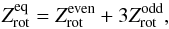 (2)where
![\begin{eqnarray} Z_{\mathrm{rot}}^{\mathrm{even}} & = & \sum_{j\,=\,0,2,4...} (2 j + 1) \exp \left[ -\frac{j(j+1)\theta_{\mathrm{rot}}}{T}\right] ,\\ Z_{\mathrm{rot}}^{\mathrm{odd}} & = & \sum_{j\,=\,1,3,5...} (2 j + 1) \exp \left[ -\frac{j(j+1)\theta_{\mathrm{rot}}}{T}\right] , \end{eqnarray}](/articles/aa/full_html/2014/03/aa22855-13/aa22855-13-eq18.png) and
θrot = 85.32 K is the rotational
excitation temperature.
and
θrot = 85.32 K is the rotational
excitation temperature.
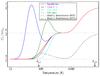 |
Fig. 1 Heat capacity for molecular hydrogen using different ortho:para ratios (see legend for details). θrot = 85.32 K and θvib = 5984.48 K are the rotational and vibrational excitation temperatures, respectively. The black dashed curve represents the raw model from Black & Bodenheimer (1975), and the black solid curve is the modified Black & Bodenheimer (1975) formula (see text). |
The choice of OPR has a direct impact on the heat capacity of the gas. Figure 1 displays the heat capacity of H2 at constant volume CV as a function of temperature for different treatments of ortho- and para-hydrogen (see for instance Balian 2007 for the computation of CV). The blue curve represents the heat capacity assuming thermal equilibrium at all temperatures, while the red curve is obtained assuming a constant 3:1 OPR. For completeness, we have also included the green and cyan curves representing the pure para and pure ortho cases, respectively. Finally, we have also plotted the model by Black & Bodenheimer (1975), which presents two peculiarities. The first is that if we use the formula as written in their Eq. (11), we get the dashed curve, which is clearly wrong and also inconsistent with their Fig. 1. To recover the correct shape for the CV curve, it was necessary to change the rotational contribution from (θrot/Tm)2f(Tm) to simply f(Tm); this yields the modified (*) black solid line in Fig. 1. The second point is that they explicitely write that their Eq. (13) holds for the case where the ortho and para states are in equilibrium at all temperatures, yet their curve resembles a 3:1 ratio much more than the equilibrium model in Fig. 1. It should also be noted that Boley et al. (2007) points out that Black & Bodenheimer (1975) used an inadequate formula to calculate the internal energy, e = CVT, while the correct definition is CV = de/dT. The first relation is valid only when CV does not depend on the temperature, and thus results in erroneous thermodynamic behaviour.
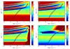 |
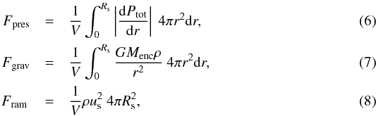
Fig. 2 Thermal evolution using EOS A (black; 3:1 OPR), EOS B (magenta; equilibrium OPR), and EOS C (grey; Saumon et al. 1995). The effective ratio of specific heats γeff is displayed in colour in the background for EOSs A, B, and C in panels a), b), and c), respectively. The region in the lower right corner of panel c) delineated by the dotted white line indicates the area of the (ρ,T) space where the values in the EOS table cannot be trusted. In panel d), the Rosseland mean opacity displayed in the background. |
Simulation parameters.
Finally for comparison purposes, we also used a third EOS (C) by Saumon et al. (1995) (and its extension to low densities; see Vaytet et al. 2013) that models the properties of the same mixture of gas but also includes non-ideal effects at high densities. It assumes an equilibrium ratio of ortho:para hydrogen and should behave very similarly to EOS B, at least at low-to-moderate densities.
3. Results
3.1. Thermal evolution
Three simulations were carried out; run 1 was performed using the fixed 3:1 EOS A, run 2
using the equilibrium EOS B, and run 3 using the Saumon et
al. (1995) EOS C (see Table 1). The
simulations were stopped when the temperature at the centre of the grid reached 30 000 K.
Figure 2 shows the thermal evolution of the gas at
the centre of the grid for all three runs (solid lines). The effective ratio of specific
heats γeff of EOSs A, B, and C are displayed in
colour in the background of panels a, b, and c, respectively. In panel d, the colour
background is used to represent the Rosseland mean opacity κR. We defined
 , where ρ, cS, and
P are the
gas density, sound speed, and pressure, respectively.
, where ρ, cS, and
P are the
gas density, sound speed, and pressure, respectively.
It can be clearly seen that using a different treatment of ortho- and para-hydrogen leads to significant differences in the thermal evolution of the collapsing core. Runs 1 and 2 show an identical evolution until the gas temperature reaches ~35 K, at which point the two curves fork, with run 2 entering lower temperatures due to a drop in adiabatic index; a light blue trench is clearly visible in panel b between 30 and 80 K; and γeff remains constant in panel a all the way up to 80 K. Different treatments of ortho- and para-hydrogen is therefore the origin of the discrepancies between the thermal evolutions of Tomida et al. (2013) and Vaytet et al. (2013).
In addition, we note that while the variations in dust and gas opacities (destruction of different dust species, sharp rise in atomic gas opacities at high temperatures) will have an impact on the transport of radiative flux (see Vaytet et al. 2013), they do not seem to affect the thermal evolution of the collapsing system to any great extent.
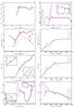 |
Fig. 3 Evolutions of the collapsing systems as a function of central density and time using EOS A (black), EOS B (magenta), and EOS C (grey). a), b) Normalised force differential ΔF between total pressure Fpres, gravity Fgrav, and ram pressure Fram (integrated over the volume of the first core) as a function of central density. The green dotted ΔF = 0 line represents hydrostatic equilibrium. c) The separate force components from gravity Fgrav (solid), gas pressure Fgas (dashed), radiation pressure Frad (dotted), and ram pressure Fram (dot-dash) as a function of central density. d) Central density as a function of time. e) Central temperature as a function of central density. f) Central temperature as a function of time. g) Adiabatic index along the thermal tracks from panel e). h) Adiabatic index at the centre of the grid as a function of time. The time of first core formation t0 is assumed to be when the central density reaches 10-13 g cm-3. In all panels, two thermal bounces are labelled ① and ② (see text). |
The thermal evolutions are displayed in more detail in Fig. 3. Panel e again shows the density of the gas at the centre of the grid as a function of its temperature, with a couple of insets revealing more of the curves’ features. Inset i first unveils the absence of a bounce1 in run 1 compared to runs 2 and 3 (the bounce is labelled ①), while on the other hand, inset j shows bounce ②, which is apparently only present in run 1. Run 1 seems to be sharply forced (by some strange/unknown mechanism) to re-join the thermal track of the last two runs for a short time, right before the onset of the second collapse. Panel g displays the evolution of γeff along the thermal tracks. The difference between the fixed ratio and equilibrium treatment of ortho- and para-hydrogen is clearly visible for densities in the range 10-12 < ρ < 10-9 (g cm-3), and bounces ① and ② are again highlighted in insets k and l, respectively.
To determine the origin of these thermal oscillations, we have computed the different
forces acting on the fluid and combined them into a normalised criterion for hydrostatic
equilibrium of the first core 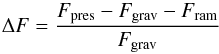 (5)where
 and
and
 ,
Rs, and us are the first
core volume, the accretion shock radius, and the gas velocity just upstream of the
accretion shock, respectively. The total pressure Ptot is the sum
of the gas pressure Pgas and the radiative pressure
Prad. The force differential
ΔF as a
function of central density is shown in Fig. 3a (the
curves are only plotted once the first core has formed, we have assumed this happens at
t0 = 192 Kyr ≃ 1.01 tff,
when the density at the centre of the grid exceeds 10-13 g cm-3), with
an inset in panel b zooming on the detail of the first hydrostatic core. For low
densities, the total pressure force Fpres is clearly over-powered by the
gravity (Fgrav) and ram pressure (Fram) forces.
(We consider the ram pressure to be the force applied by the infalling envelope’s gas onto
the surface of the first core.) Then, as the gas heats up, Ptot rises and
brings the system very close to hydrostatic equilibrium. All three runs overshoot the
ΔF = 0 mark
and show subsequent oscillations that die down and disappear for densities above
10-8.5 g cm-3. Panel c also shows the
different contributions to ΔF, revealing that the radiative pressure plays a
very minor role, while the ram pressure is important at the first core formation but
diminishes once the core has reached quasi-equilibrium.
,
Rs, and us are the first
core volume, the accretion shock radius, and the gas velocity just upstream of the
accretion shock, respectively. The total pressure Ptot is the sum
of the gas pressure Pgas and the radiative pressure
Prad. The force differential
ΔF as a
function of central density is shown in Fig. 3a (the
curves are only plotted once the first core has formed, we have assumed this happens at
t0 = 192 Kyr ≃ 1.01 tff,
when the density at the centre of the grid exceeds 10-13 g cm-3), with
an inset in panel b zooming on the detail of the first hydrostatic core. For low
densities, the total pressure force Fpres is clearly over-powered by the
gravity (Fgrav) and ram pressure (Fram) forces.
(We consider the ram pressure to be the force applied by the infalling envelope’s gas onto
the surface of the first core.) Then, as the gas heats up, Ptot rises and
brings the system very close to hydrostatic equilibrium. All three runs overshoot the
ΔF = 0 mark
and show subsequent oscillations that die down and disappear for densities above
10-8.5 g cm-3. Panel c also shows the
different contributions to ΔF, revealing that the radiative pressure plays a
very minor role, while the ram pressure is important at the first core formation but
diminishes once the core has reached quasi-equilibrium.
The overshoots in panels a and b indicate that all three runs should display a bounce ① in their thermal tracks; so why is it not the case for run 1? The temporal evolutions of the central densities and temperatures can provide an answer. Indeed, panels d and f show that the clouds in runs 2 and 3 collapse faster than in run 1 (due to the drop in γeff; see Figs 2b and 3g). As a result, the heating at the centre of the core is very sudden when the value of γeff recovers the classical diatomic value of 7/5, causing a sharp oscillation in ΔF, i.e. bounce ① in panel b. Things are a lot smoother for run 1, with a much steadier increase in central density and temperature. Small oscillations are seen in panels d and f (as indeed was noticed by Tomida et al. 2013 in their simulations), but nothing large enough to induce a detectable oscillation in the thermal track. In addition, the overshoot in runs 2 and 3 is actually higher than for run 1.
In the case of bounce ②, what looked like a relatively violent event in panels e and g, and by extension also in inset m of panel b, turns out to be a relatively slow oscillation that can be seen in panel f. The small region of the (ρ,T) space where all three curves overlapped right before the start of the second collapse in fact represents quite a substantial part of the first core’s lifetime. Between 600 and 1100 years after the formation of the first core, there is a lengthy transition period (see Vaytet et al. 2013) during which the central density and temperature increase very slowly, and the core continues to accrete mass. Run 1 is not forced to re-join the thermal track of runs 2 and 3 (as first suggested by panel e), all runs simply reach the same state of hydrostatic equilibrium where they remain for ~500 years, a phase during which their early evolution is forgotten before the second stage of the collapse is entered. The short region where all the curves overlap just after bounce ② in inset j actually corresponds to a relatively long period of time in panels d and f.
This was confirmed by running another three simulations for which we halved the parent cloud size (runs 4, 5, and 6 in Table 1). A smaller cloud radius for the same cloud mass produced thermal evolutions without a transition period in Vaytet et al. (2013). Figure 4 shows the thermal evolutions for these new simulations (same colour coding for the different EOSs). The calculations using an equilibrium OPR still show a bounce around ~10-10−10-9 g cm-3 in panel a, but no flat plateau is visible in panel b. There is also no lengthy hydrostatic period in the evolution of the fixed OPR run. As a consequence the thermal track never meets the tracks from the other two runs again, it instead remains at higher temperatures throughout the rest of the simulation. This inevitably has an effect on the properties of the second core, which is formed at lower densities, and is consequently larger in size. It is also higher in mass, as reported in Table 1.
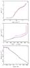 |
Fig. 4 Three additional simulations with a parent cloud half the size, using EOS A (black), EOS B (magenta), and EOS C (grey). a) Central temperature as a function of central density. b) Central density as a function of time (t0 = 62 Kyr ≃ 0.997 tff). c) Density radial profiles. |
Finally, during the second phase of the collapse2, Fig. 3a shows that the gravitational force once again overcomes the failing thermal pressure. (The thermal energy is being consumed by the dissociation of the H2 molecules.) Hydrostatic equilibrium is recovered at the end of the second collapse, again with some overshoot. The shape of the curves suggests that more oscillations are to come, but the simulations were stopped before these became apparent. (Once the second core is formed, the computational time required to advance the simulations further becomes colossal.)
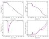 |
Fig. 5 Radial profiles of the gas density a), temperature b), velocity c), and entropy d). As in Fig. 2, the black, magenta, and grey curves represent runs 1, 2, and 3, respectively. |
3.2. Radial profiles
While the OPR has a significant impact on the thermal evolution of the collapsing cores, it does not seem to affect the radial profiles of their gas quantities much, as shown in Fig. 5. The gas density, temperature, and velocity profiles of the first two runs are extremely similar for most of the system. A small difference (~25%) in the second core radius (see Table 1) and an even smaller difference in central density (for the same temperature) are observed. The entropy profiles differ somewhat more because the partition functions of H2 are different.
In the case of more unstable clouds (runs 4−6), the first cores remain insensitive to the choice of OPR, while some moderately greater differences arise in the second core’s characteristics. As mentioned in Sect. 3.1, the thermal tracks of simulations using EOS A probe higher temperatures compared to runs with EOS B (for the same central density), and the second core consequently forms at lower densities, with a larger radius. The core is ~40% larger in size and mass, and this is clearly visible in Fig. 4c (see also Table 1). We must, however, note here that we are comparing second-core profiles at the onset of protostellar formation, and the differences reported here may only be short-lived.
These variations (for both marginally unstable and more unstable clouds) are, however, probably much too small (and very transient?) to be detected in observations, and measuring core masses, radii, temperatures, or velocity profiles cannot be used to differentiate between a fixed or an equilibrium ratio of ortho:para hydrogen. Moreover, the disparities occur at the second Larson core, which is deeply embedded inside the first code and extremely difficult (if not impossible) to observe directly. The only feasible (albeit difficult) method of disentangling the two remains the study of chemistry in the system through spectroscopic observations.
At high densities, small differences start to appear between runs 2 and 3. Indeed, Fig. 2c shows a departure in γeff at high densities from ideality; this is a region where plasma effects become important (Saumon et al. 1995). This also results in a slightly higher density for the same temperature (Fig. 5a). The subsequent evolution of the second Larson core will probably be affected by non-ideal effects to some extent, but the results of this paper suggest that the ideal mixture of H and He is a valid description of the state of the gas during the very early stages of star formation.
3.3. Confusion in other studies
In Vaytet et al. (2013), after comparing several studies of gravitational cloud core collapse, the authors concluded that the OPR was not the main factor contributing to differences in the thermal evolution of the collapsing bodies. The five studies compared were the works of Masunaga & Inutsuka (2000), Whitehouse & Bate (2006), Stamatellos et al. (2007), Tomida et al. (2013), and Vaytet et al. (2013). The argument was that works that made use of equilibrium OPR resembled ones that assume non-equilibrium OPR and vice-versa. We now suspect that the OPR is indeed responsible for the two different thermal tracks and that the misled conclusions of Vaytet et al. (2013) are the result of confusing terminology employed in the papers.
Masunaga & Inutsuka (2000) and Vaytet et al. (2013) both make use of the Saumon et al. (1995) EOS, and it is thus natural that they display very similar thermal evolutions (a thermal track equivalent to run 3 in the present paper). Tomida et al. (2013) use the non-equilibrium fixed 3:1 EOS of the present paper, and consequently shows a thermal evolution that strongly resembles run 1 (and run 4 even more). Whitehouse & Bate (2006) say that they use the model of Black & Bodenheimer (1975), which claims that equilibrium is assumed at all temperatures, yet the thermal path taken by their collapsing cloud echoes the non-equilibrium track. As discussed in Sect. 2.2, we believe that the heat capacity of the Black & Bodenheimer (1975) EOS is in fact much closer to a non-equilibrium model. They adopt the 3:1 OPR in their recent works (e.g. Bate 2011) and the evolution of the non-rotating model is qualitatively consistent with the results of our non-equilibrium models. Finally, the simulation of Stamatellos et al. (2007) follows an equilibrium-like path, even though they state that their EOS assumes a fixed 3:1 OPR. Interestingly, in a later paper (Stamatellos & Whitworth 2009), they use the same numerical method, reporting that they assume that ortho- and para-hydrogen are in equilibrium. It is not clear whether they have changed their ortho-para strategy between the two studies, or if they simply made a mistake in their 2007 paper; their thermal evolution suggests the latter.
We hope this section has cleared up any confusion there may have been between the different studies of gravitational collapse using radiation hydrodynamics.
4. Conclusions
We performed simulations of the gravitational collapse of a dense cloud core using radiation hydrodynamics and distinct gas EOSs using two different treatments of the OPR: either a fixed 3:1 OPR or an equilibrium ratio. The choice of OPR has a significant impact on the thermal evolutions of the collapsing cores. Systems in simulations using an equilibrium ratio collapse faster at early times, when a drop in γeff (see Figs. 2b and 3g) corresponding to an increase in CV (see Fig. 1) facilitates the collapse. This yields rapid heating once γeff starts to increase again around T ~ 100 K, generating marked oscillations around hydrostatic equilibrium, to the point where the core expands for a short time right after its formation before resuming its contraction. In the case of a fixed 3:1 OPR, the core’s evolution is a lot smoother. The transition from a monatomic γeff = 5/3 to a diatomic value of 7/5 is monotonous, the thermal support more important, and hydrostatic equilibrium is reached earlier in terms of central density. By contrast, the radial profiles of the cores (gas density, velocity, temperature) were not greatly affected by the choice of OPR. The first core radii were virtually identical, while only moderate differences in the second core radius and density were observed.
We studied two different initial configurations: marginally unstable and positively unstable parent clouds. In the first case, once the simulations (both fixed and equilibrium OPR) have reached the first hydrostatic equilibrium, they evolve along the same thermal tracks, with they central densities and temperatures slowly rising until the second phase of the collapse is triggered by the dissociation of the H2 molecules, eventually forming very similar second cores. The slow transition period between first and second collapse was absent from the more unstable cloud calculations, and this implied that the collapsing systems using different OPRs did not have time to relax towards the same adiabat and consequently did not embark on the second collapse at the same densities. Fixed OPR simulations yielded an increase of ~40% in second core mass and size. We wish to emphasise here that these differences apply to the newly formed second core, the initial protostellar seed, which will subsequently grow in size and mass at a considerable rate thanks to the immense accretion rate at the core’s border. It is very possible that the initial difference of 40% will later become washed out, once the protostar is well into its evolution towards becoming a young star. We must further acknowledge that our spherically symmetric simulations do not include any three-dimensional effects, such as the launching of outflows and creation of accretions discs, which play an important role in star formation.
It is finally not clear which is the best OPR to adopt for simulations of low-mass star formation. While observations suggest that the OPR is far from equilibrium in dark clouds (Pagani et al. 2011; Dislaire et al. 2012), Flower & Watt (1984) have shown that under typical molecular cloud conditions (n ~ 100−1000 cm-3), the time when ortho:para equilibrium is reached is of the order of 1 Myr. This is of course five to ten times longer than the free-fall time of the core we are modelling, but this core is formed as a result of turbulence in the molecular cloud, which spawns over-densities that eventually become gravitationally unstable. The collapse will begin long after the formation of the molecular cloud, which has a typical lifetime of ~10 Myr, and it is thus very possible that at the onset of the collapse, ortho:para equilibrium has already been reached. In summary, it is not obvious which ortho:para strategy (fixed ratio or equilibrium) best represents the initial conditions of star formation. Nevertheless, if one is solely interested in the final properties of the cores when they are formed, it may not matter much which OPR is used. On the other hand, if one’s focus lies primarily on the evolution of the first core3, the choice of OPR is of substance. In addition, as Boley et al. (2007) point out, the stability of massive circumstellar disks can also be considerably affected by the OPR. The typical temperature range found inside protoplanetary discs (apart from the inner disc regions) coincides with the area where the heat capacities given by the fixed and equilibrium OPR differ the most (20−300 K; see Pinte et al. 2009, for instance). Accretion discs formed using an equilibrium OPR may have a lower temperature and could in principle be more prone to fragmentation, but this is pure speculation. We will refrain from drawing any conclusions here before having run the simulations in 3D, since many additional effects (magnetic fields, angular momentum) also come into the picture, possibly weakening the importance of the OPR.
Period of time during which the core is thermally supported, before collapse resumes when the core has accreted enough mass (see Vaytet et al. 2013).
Acknowledgments
The research leading to these results has received funding from the European Research Council under the European Community’s Seventh Framework Programme (FP7/2007−2013 Grant Agreement No. 247060). K.T. is supported by Japan Society for the Promotion of Science (JSPS) Postdoctoral Fellowship for Research Abroad. The authors would also like to thank the anonymous referee for useful comments.
References
- Balian, R. 2007, From Microphysics to Macrophysics: Methods and Applications of Statistical Physics, Vol. I, Theoretical and Mathematical Physics (Berlin, Heidelberg: Springer-Verlag) [Google Scholar]
- Bate, M. 2011, MNRAS, 417, 2036 [NASA ADS] [CrossRef] [Google Scholar]
- Black, D. C., & Bodenheimer, P. 1975, ApJ, 199, 619 [NASA ADS] [CrossRef] [Google Scholar]
- Boley, A. C., Hartquist, T. W., Durisen, R. H., & Michael, S. 2007, ApJ, 656, L89 [NASA ADS] [CrossRef] [Google Scholar]
- Carlson, B. E., Lacis, A. A., & Rossow, W. B. 1992, ApJ, 393, 357 [NASA ADS] [CrossRef] [Google Scholar]
- Crabtree, K. N., Indriolo, N., Kreckel, H., Tom, B. A., & McCall, B. J. 2011, ApJ, 729, 15 [NASA ADS] [CrossRef] [Google Scholar]
- Dalgarno, A., Black, J. H., & Weisheit, J. C. 1973, Astroph. Lett., 14, 77 [Google Scholar]
- Decampli, W. M., Cameron, A. G. W., Bodenheimer, P., & Black, D. C. 1978, ApJ, 223, 854 [NASA ADS] [CrossRef] [Google Scholar]
- Dislaire, V., Hily-Blant, P., Faure, A., et al. 2012, A&A, 537, A20 [NASA ADS] [CrossRef] [EDP Sciences] [Google Scholar]
- Dubroca, B., & Feugeas, J.-L. 1999, C. R. Acad. Sci. Paris, 329, 915 [Google Scholar]
- Duley, W., & Williams, D. A. 1984, Interstellar Chemistry (London: Academic Press) [Google Scholar]
- Duley, W., & Williams, D. A. 1993, MNRAS, 260, 37 [NASA ADS] [CrossRef] [Google Scholar]
- Dyson, J. E., & Williams, D. A. 1997, The Physics of the Interstellar Medium, 2nd edn. (Bristol: Institute of Physics) [Google Scholar]
- Flower, D. R., & Watt, G. D. 1984, MNRAS, 209, 25 [NASA ADS] [Google Scholar]
- Flower, D. R., Pineau Des Forêts, G., & Walmsley, C. M. 2006, A&A, 449, 621 [NASA ADS] [CrossRef] [EDP Sciences] [Google Scholar]
- Galli, D., Walmsley, M., & Gonçalves, J. 2002, A&A, 394, 275 [NASA ADS] [CrossRef] [EDP Sciences] [Google Scholar]
- Gavilan, L., Vidali, G., Lemaire, J. L., et al. 2012, ApJ, 760, 35 [NASA ADS] [CrossRef] [Google Scholar]
- Habart, E., Walmsley, M., Verstraete, L., et al. 2005, Space Sci. Rev., 119, 71 [Google Scholar]
- Harrison, A., Puxley, P., Russell, A., & Brand, P. 1998, MNRAS, 297, 624 [NASA ADS] [CrossRef] [Google Scholar]
- Hoban, S., Reuter, D. C., Mumma, M. J., & Storrs, A. D. 1991, ApJ, 370, 228 [NASA ADS] [CrossRef] [Google Scholar]
- Larson, R. B. 1969, MNRAS, 145, 271 [NASA ADS] [CrossRef] [Google Scholar]
- Levermore, C. D. 1984, JQSRT, 31, 149 [NASA ADS] [CrossRef] [Google Scholar]
- Massie, S. T., & Hunten, D. M. 1982, Icarus, 49, 213 [NASA ADS] [CrossRef] [Google Scholar]
- Masunaga, H., & Inutsuka, S.-I. 2000, ApJ, 531, 350 [NASA ADS] [CrossRef] [Google Scholar]
- Neufeld, D. A., Melnick, G. J., & Harwit, M. 1998, ApJ, 506, L75 [NASA ADS] [CrossRef] [Google Scholar]
- Neufeld, D. A., Melnick, G. J., Sonnentrucker, P., et al. 2006, ApJ, 649, 816 [NASA ADS] [CrossRef] [Google Scholar]
- Osterbrock, D. E. 1962, ApJ, 136, 359 [NASA ADS] [CrossRef] [Google Scholar]
- Pagani, L., Vastel, C., Hugo, E., et al. 2009, A&A, 494, 623 [NASA ADS] [CrossRef] [EDP Sciences] [Google Scholar]
- Pagani, L., Roueff, E., & Lesaffre, P. 2011, ApJ, 739, L35 [NASA ADS] [CrossRef] [Google Scholar]
- Pinte, C., Harries, T. J., Min, M., et al. 2009, A&A, 498, 967 [NASA ADS] [CrossRef] [EDP Sciences] [Google Scholar]
- Raich, J. C., & Good, R. H., Jr. 1964, ApJ, 139, 1004 [NASA ADS] [CrossRef] [Google Scholar]
- Rodríguez-Fernández, N. J., Martín-Pintado, J., de Vicente, P., et al. 2000, A&A, 356, 695 [NASA ADS] [Google Scholar]
- Saumon, D., Chabrier, G., & van Horn, H. M. 1995, ApJS, 99, 713 [NASA ADS] [CrossRef] [Google Scholar]
- Schwabl, F. 2006, Statistical Mechanics (Berlin: Springer) [Google Scholar]
- Sears, F. W., & Salinger, G. L. 1975, Thermodynamics, kinetic theory, and statistical thermodynamics (Addison-Wesley Pub. Co.) [Google Scholar]
- Smith, M. D., Davis, C. J., & Lioure, A. 1997, A&A, 327, 1206 [NASA ADS] [Google Scholar]
- Souers, P. C. 1986, Hydrogen Properties for Fusion Energy, Chap. 24 (Berkeley: University of California Press) [Google Scholar]
- Stamatellos, D., Whitworth, A. P., Bisbas, T., & Goodwin, S. 2007, A&A, 475, 37 [NASA ADS] [CrossRef] [EDP Sciences] [Google Scholar]
- Stamatellos, D., & Whitworth, A. P. 2009, MNRAS, 400, 1563 [NASA ADS] [CrossRef] [Google Scholar]
- Takahashi, J. 2001, ApJ, 561, 254 [NASA ADS] [CrossRef] [Google Scholar]
- Takayanagi, K., Sakimoto, K., & Onda, K. 1987, ApJ, 318, L81 [NASA ADS] [CrossRef] [Google Scholar]
- Tomida, K., Tomisaka, K., Matsumoto, T., et al. 2013, ApJ, 763, 6 [NASA ADS] [CrossRef] [Google Scholar]
- Vaytet, N., Audit, E., Chabrier, G., Commerçon, B., & Masson, J. 2012, A&A, 543, A60 [NASA ADS] [CrossRef] [EDP Sciences] [Google Scholar]
- Vaytet, N., Chabrier, G., Audit, E., et al. 2013, A&A, 557, A90 [NASA ADS] [CrossRef] [EDP Sciences] [Google Scholar]
- Wannier, G. H. 1966, Statistical Physics (New York: John Wiley & Sons) [Google Scholar]
- Whitehouse, S. C., & Bate, M. R. 2006, MNRAS, 367, 32 [NASA ADS] [CrossRef] [Google Scholar]
All Tables
All Figures
|
Fig. 1 Heat capacity for molecular hydrogen using different ortho:para ratios (see legend for details). θrot = 85.32 K and θvib = 5984.48 K are the rotational and vibrational excitation temperatures, respectively. The black dashed curve represents the raw model from Black & Bodenheimer (1975), and the black solid curve is the modified Black & Bodenheimer (1975) formula (see text). |
| In the text | |
|
Fig. 2 Thermal evolution using EOS A (black; 3:1 OPR), EOS B (magenta; equilibrium OPR), and EOS C (grey; Saumon et al. 1995). The effective ratio of specific heats γeff is displayed in colour in the background for EOSs A, B, and C in panels a), b), and c), respectively. The region in the lower right corner of panel c) delineated by the dotted white line indicates the area of the (ρ,T) space where the values in the EOS table cannot be trusted. In panel d), the Rosseland mean opacity displayed in the background. |
| In the text | |
|
Fig. 3 Evolutions of the collapsing systems as a function of central density and time using EOS A (black), EOS B (magenta), and EOS C (grey). a), b) Normalised force differential ΔF between total pressure Fpres, gravity Fgrav, and ram pressure Fram (integrated over the volume of the first core) as a function of central density. The green dotted ΔF = 0 line represents hydrostatic equilibrium. c) The separate force components from gravity Fgrav (solid), gas pressure Fgas (dashed), radiation pressure Frad (dotted), and ram pressure Fram (dot-dash) as a function of central density. d) Central density as a function of time. e) Central temperature as a function of central density. f) Central temperature as a function of time. g) Adiabatic index along the thermal tracks from panel e). h) Adiabatic index at the centre of the grid as a function of time. The time of first core formation t0 is assumed to be when the central density reaches 10-13 g cm-3. In all panels, two thermal bounces are labelled ① and ② (see text). |
| In the text | |
|
Fig. 4 Three additional simulations with a parent cloud half the size, using EOS A (black), EOS B (magenta), and EOS C (grey). a) Central temperature as a function of central density. b) Central density as a function of time (t0 = 62 Kyr ≃ 0.997 tff). c) Density radial profiles. |
| In the text | |
|
Fig. 5 Radial profiles of the gas density a), temperature b), velocity c), and entropy d). As in Fig. 2, the black, magenta, and grey curves represent runs 1, 2, and 3, respectively. |
| In the text | |
Current usage metrics show cumulative count of Article Views (full-text article views including HTML views, PDF and ePub downloads, according to the available data) and Abstracts Views on Vision4Press platform.
Data correspond to usage on the plateform after 2015. The current usage metrics is available 48-96 hours after online publication and is updated daily on week days.
Initial download of the metrics may take a while.