| Issue |
A&A
Volume 563, March 2014
|
|
|---|---|---|
| Article Number | A74 | |
| Number of page(s) | 9 | |
| Section | Interstellar and circumstellar matter | |
| DOI | https://doi.org/10.1051/0004-6361/201322845 | |
| Published online | 13 March 2014 | |
The deuterium fractionation of water on solar-system scales in deeply-embedded low-mass protostars⋆
1 Centre for Star and Planet Formation, Natural History Museum of Denmark, University of Copenhagen, Øster Voldgade 5–7, 1350 Copenhagen K, Denmark
e-mail: This email address is being protected from spambots. You need JavaScript enabled to view it.
2 Niels Bohr Institute, University of Copenhagen, Juliane Maries Vej 30, 2100 Copenhagen Ø, Denmark
3 Leiden Observatory, Leiden University, PO Box 9513, 2300 RA Leiden, The Netherlands
4 Max-Planck Institute für extraterrestrische Physik (MPE), Giessenbachstrasse, 85748 Garching, Germany
Received: 14 October 2013
Accepted: 3 February 2014
Abstract
Context. The chemical evolution of water through the star formation process directly affects the initial conditions of planet formation. The water deuterium fractionation (HDO/H2O abundance ratio) has traditionally been used to infer the amount of water brought to Earth by comets. Measuring this ratio in deeply-embedded low-mass protostars makes it possible to probe the critical stage when water is transported from clouds to disks in which icy bodies are formed.
Aims. We aim to determine the HDO/H2O abundance ratio in the warm gas in the inner 150 AU for three deeply-embedded low-mass protostars NGC 1333-IRAS 2A, IRAS 4A-NW, and IRAS 4B through high-resolution interferometric observations of isotopologues of water.
Methods. We present sub-arcsecond resolution observations of the 31,2−22,1 transition of HDO at 225.89672 GHz in combination with previous observations of the 31,3−22,0 transition of H218O at 203.40752 GHz from the Plateau de Bure Interferometer toward three low-mass protostars. The observations have similar angular resolution (0.̋7–1.̋3), probing scales R ≲ 150 AU. In addition, observations of the 21,1−21,2 transition of HDO at 241.561 GHz toward IRAS 2A are presented to constrain the excitation temperature. A direct and model independent HDO/H2O abundance ratio is determined for each source and compared with HDO/H2O ratios derived from spherically symmetric full radiative transfer models for two sources.
Results. From the two HDO lines observed toward IRAS 2A, the excitation temperature is found to be Tex = 124 ± 60 K. Assuming a similar excitation temperature for H218O and all sources, the HDO/H2O ratio is 7.4 ± 2.1 × 10⁻⁴ for IRAS 2A, 19.1 ± 5.4 × 10⁻⁴ for IRAS 4A-NW, and 5.9 ± 1.7 × 10⁻⁴ for IRAS 4B. The abundance ratios show only a weak dependence on the adopted excitation temperature. The abundances derived from the radiative transfer models agree with the direct determination of the HDO/H2O abundance ratio for IRAS 16293-2422 within a factor of 2–3, and for IRAS 2A within a factor of 4; the difference is mainly due to optical depth effects in the HDO line.
Conclusions. Our HDO/H2O ratios for the inner regions (where T > 100 K) of four young protostars are only a factor of 2 higher than those found for pristine, solar system comets. These small differences suggest that little processing of water occurs between the deeply embedded stage and the formation of planetesimals and comets.
Key words: astrochemistry / stars: formation / ISM: abundances / protoplanetary disks / stars: general
Based on observations carried out with the IRAM Plateau de Bure Interferometer.
© ESO, 2014
1. Introduction
Water is a very important molecule through all stages of star and planet formation. In dense clouds, it is one of the dominant reservoirs of oxygen, both as a gas at high temperatures or as ice in grain mantles in cold regions. It also aids in the sticking of grains outside the snow line, and is crucial for the emergence of life on Earth. This makes it vital to understand the chemical evolution of water during the different stages of star formation, and to identify the mechanism by which it was brought to the Earth and Earth-like planets.
One way to gain insight into the chemical evolution of water is to compare the level of deuterium fractionation in water (the HDO/H2O ratio) at various stages of star and planet formation. In our own solar system, several measurements of the HDO/H2O ratio1 exist for long-period comets from the Oort cloud (Mumma & Charnley 2011, and references therein). Up until recently the mean HDO/H2O ratio for these objects was 6.4 ± 1.0 × 10⁻⁴ (Villanueva et al. 2009; Jehin et al. 2009), significantly above the value for the Earth’s oceans 3.114 ±0.002 × 10⁻⁴ (VSMOW2, de Laeter et al. 2003, and references therein). Both values are well above the protosolar nebula value of 2 × D/H = 0.42 ± 0.08 × 10⁻⁴ (Geiss & Gloeckler 1998; Lellouch et al. 2001) indicating that deuterium fractionation of water has taken place. Because of the observed difference between the Earth and comets, it has been argued that only a small fraction (≤10%) of the Earth’s water could have its origin in comets (Morbidelli et al. 2000; Drake 2005).
The Jupiter family comet Hartley 2 observed with the Herschel Space Observatory was found to have a HDO/H2O ratio of 3.2 ± 0.5 × 10⁻⁴, significantly lower than the value for Oort cloud comets, and comparable to VSMOW (Hartogh et al. 2011). Jupiter family comets have relatively short periods (≲20 years), with orbits more or less confined to the ecliptic plane, and originate in the Kuiper belt (Duncan et al. 2004; Mumma & Charnley 2011). Oort cloud comets have longer periods, orbits distributed isotropically, and originate in the Oort cloud. In 2012 Bockelée-Morvan et al. observed the Oort cloud comet Garradd with Herschel and deduced a HDO/H2O ratio of 4.12 ± 0.44 × 10⁻⁴. This is significantly lower than previous measurements of Oort cloud comets. Recently, Lis et al. (2013) measured the HDO/H2O ratio in the Jupiter family comet Honda-Mrkos-Pajdusakov (HMP) using Herschel to <4.0×10⁻⁴. These latest measurements indicate a certain range in the water deuterium fractionation in comets, possibly dependent on the precise formation location and subsequent migration, in which Jupiter family comets no longer have a distinctly lower HDO/H2O ratio than Oort cloud comets. Simulations suggest that the deuterium fractionation in the protosolar nebula disk increases with distance from the forming sun (Hersant et al. 2001; Kavelaars et al. 2011) – but whether the observed ratios are consistent with these simulations is still unclear.
Measurements of the water deuterium fractionation toward protostars provide a different perspective. By determining the HDO/H2O ratio of material that enters protoplanetary disks, it is possible to set the initial level of deuterium fractionation in comet forming zones as input for any subsequent evolutionary models. So far, determinations of HDO/H2O have given a wide range of results. Parise et al. (2003) used ground-based infrared observations of the stretching bands of OH and OD in water ice in the cold outer parts of protostellar envelopes and found upper limits ranging from 0.5% to 2% for the HDO/H2O ratios. Studies using gaseous HDO lines differ in the interpretation, with cold HDO/H2O ratios derived from single-dish data ranging from cometary values (2 × 10⁻⁴, Stark et al. 2004), to a few × 10-2 (Parise et al. 2005; Liu et al. 2011; Coutens et al. 2012). In the inner warm (T > 100 K) region, HDO/H2O ratios ≥1% have also been inferred based on analysis of many HDO and water lines (Eu up to 450 K) (Liu et al. 2011; Coutens et al. 2012). In contrast, Jørgensen & van Dishoeck (2010b) derived a HDO/ H2O ratio toward the Class 0 protostar NGC 1333-IRAS 4B of <6.4 × 10⁻⁴ from the interferometric Submillimeter Array (SMA) and Plateau de Bure (PdBI) observations, up to two orders of magnitude lower.
There are two main issues with determining the water abundances in the warm gas in the inner few hundred au. First, the relatively large beam sizes (>10′′) of single-dish telescopes are more sensitive to extended emission than the small ~1″ scales on which the warm water is found. Second, many observed water lines suffer from high optical depths, even for isotopologues, making it difficult to infer reliable column densities and abundances for H2O in the warm (>100 K) gas. Indeed, Visser et al. (2013) find that the 31,2 − 30,3 lines (Eu = 249 K) of H O, H
O, H O and even H
 O observed by the HIFI instrument (de Graauw et al. 2010) aboard Herschel probably show optically thick emission on R ~ 100 AU scales in the well-studied Class 0 protostar NGC1333-IRAS 2A. Taking the optical depth properly into account lowers the HDO/H2O ratio for IRAS 2A from ≥0.01 to 1 × 10⁻³ (Visser et al. 2013).
Recent high-resolution interferometric ground-based observations have made it possible to estimate the abundances of both H2O and HDO in the warm gas on small scales. Jørgensen & van Dishoeck (2010a) targeted the HO 31,3 − 22,0 line at 203 GHz with PdBI, which has a much lower Einstein A coefficient than the lines observed with Herschel and thus suffers less from optical depth effects. Using SMA data of the HDO 31,2 − 22,1 transition at 225 GHz, the above mentioned HDO/H2O limit of <6.4 ×10⁻⁴ was found toward NGC 1333-IRAS 4B (Jørgensen & van Dishoeck 2010b). Coutens et al. (2013) obtained values of 4 − 30 × 10-4 for IRAS 4A and 1 − 37 × 10-4 for IRAS 4B using new Herschel data combined with the HO column densities found by Persson et al. (2012) based on interferometric data.
Taquet et al. (2013) derived the warm HDO/H2O ratios for IRAS 2A and IRAS 4A using the determinations of the HO column density from Persson et al. (2012) and lower spatial- and spectral-resolution interferometric observations targeting the HDO 42,2 − 42,3 transition (143.7 GHz, Eu = 316.2 K) together with single dish (Liu et al. 2011) observations of HDO. Using non-local thermal equilibrium (non-LTE) large velocity gradient (LVG) analysis, ratios in the range of 30 − 800 × 10-4 for IRAS 2A and 50 − 300 × 10-4 for IRAS 4A were obtained, depending on the assumed density, with the high-density (nH2 = 1 × 108 cm-3) solution giving the lowest ratios. Finally, using Atacama Large Millimeter/submillimeter Array (ALMA) and SMA observations, Persson et al. (2013) estimated the HDO/H2O ratio of the warm water toward IRAS 16293-2422 A to 9.2 ± 2.6 × 10⁻⁴.
Most of these new values, summarized in Table A.1, are significantly lower than the previous estimates of a few percentage points, indicating that the deuterium fractionation in warm water may not be as enhanced as previously thought.
In order to settle the question of the HDO/H2O abundance ratios in warm gas, we have obtained high spatial resolution interferometric observations of HDO to complement previous high quality data of HO for three sources. The observations are sensitive to scales comparable to disks (~ , R ≲ 150 AU), allowing us to determine the HDO/H2O ratio in the innermost parts of young protostars where the disk is forming.
This paper presents observations of HDO 31,2 − 22,1 at 225.9 GHz toward the three well-known deeply-embedded low-mass protostars in the NGC 1333 region of the Perseus molecular cloud (Jennings et al. 1987; Sandell et al. 1991 – IRAS 2A, IRAS 4A, and IRAS 4B in the following) at a distance of 250 pc (Enoch et al. 2006). The three sources are ideal to compare because of their similar masses, luminosities, and location (Jørgensen et al. 2006). Persson et al. (2012) presented observations of the HO 31,3 − 22,0 transition at 203.4 GHz toward the same sources. With these two datasets we can deduce a HDO/H2O ratio in the warm gas in the inner 150 AU radius using the same method and similar sensitivity and resolution as for IRAS 16293-2422, bringing the total number of low-mass protostars for which high quality data exist to four. In addition, observations of HDO 21,1 − 21,2 at 241.6 GHz toward IRAS 2A were acquired to empirically constrain the excitation temperature. The paper is laid out as follows. Section 2 describes the details of the various observations. Sections 3 and 4 present the results and analysis – including intensities, column densities, spectra, maps, and line radiative transfer modeling of the observed emission. In Sect. 5 we discuss the deduced HDO/H2O ratio and compare it to other studies of protostars and with solar system objects.
2. Observations
Three low-mass protostars, IRAS 2A, IRAS 4A, and IRAS 4B in the embedded cluster NGC 1333 were observed using the PdBI. All sources were observed with two different receiver setups. One setup was tuned to the HO 31,3 − 22,0 transition at 203.40752 GHz, for details about those observations see Jørgensen & van Dishoeck (2010a) and Persson et al. (2012). In the other setup, the receivers were tuned to the HDO 31,2−22,1 transition at 225.89672 GHz. IRAS 2A was observed in the C configuration on 27 and 28 November 2011 (8 h; including calibration) and the B configuration on 12 March 2012 (2 h). IRAS 4A and IRAS 4B were observed in track sharing mode in the B configuration on 12 March 2012 (4 h), and C on 15, 27, and 21 March and on 2 April (3 h). For IRAS 2A the combined dataset covers baselines from 15.8 to 452.0 m (11.9 to 340.5 kλ), for IRAS 4A from 15.0 to 452.0 m (11.3 to 340.5 kλ), and for IRAS 4B from 16.3 to 451.9 m (12.3 to 340.5 kλ). The correlators were set up with one unit with a bandwidth of 40 MHz (47.6 km s-1) centered on the frequency of the HDO line (225.89672 GHz), providing a spectral resolution on 460 channels of 0.087 MHz (0.104 km s-1) width3.
The data were calibrated and imaged using the CLIC and MAPPING packages, part of the IRAM GILDAS software. Regular observations of the nearby, strong quasars 0333+321, 3C84, and 2200+420 or 1749+096 were used to calibrate the complex gains and bandpass, while MWC349 and 0333+321 were observed to calibrate the absolute flux scale. During the calibration procedure integrations with significantly deviating amplitude and or phases were flagged and the continuum was subtracted before Fourier transformation of the line data.
In addition to these observations, the HDO 21,1−21,2 line at 241.56155 GHz was observed toward IRAS 2A on 7 and 17 November 2012 in the C configuration for 8 hours covering baselines from 15.5 to 175.8 m (12.5 to 141.7 kλ). The correlators were set up with one unit covering 80 MHz (89.0 km s-1) with a spectral resolution of 0.174 MHz (0.1939 km s-1) on 460 channels. The same calibration steps as described above were followed.
The resulting beam sizes using natural weighting and other parameters for the observations are given in Table 1. The field of view is roughly 22′′ (HPBW) at 225.9 GHz and the continuum sensitivity is limited by the dynamical range of the interferometer. The uncertainty in fluxes is dominated by the accuracy of the flux calibration, typically about 20%.
Parameters for the observations tuned to HDO at 225.9 GHz and 241.6 GHz.
3. Results
Both the targeted lines and the continuum are detected with high signal to noise in all three sources (Fig. 1). Elliptical Gaussian fits to the (u,v)-plane of the continuum are tabulated in Table 2. The continuum emission from the sources agrees with previous observations (e.g., Jørgensen et al. 2007; Jørgensen & van Dishoeck 2010a; Persson et al. 2012), following a power-law (Fν ∝ να) with exponents expected from thermal dust continuum emission (i.e., α ~ 2 − 3). This shows that the flux calibrations for the different observations are accurate to within roughly 20%.
Parameters of the continuum determined from elliptical Gaussian fits in the (u,v)-plane.
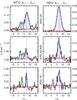 |
Fig. 1 Continuum subtracted spectra of the H |
To identify the lines, the Jet Propulsion Laboratory (JPL, Pickett et al. 1998) and the Cologne Database for Molecular Spectroscopy (CDMS, Müller et al. 2001) line-lists were queried through the Splatalogue4 interface. The molecular parameters for the lines are tabulated in Table A.2. The continuum subtracted spectra of both the HO 31,3 − 22,0 and the HDO 31,2 − 22,1 transition extracted toward the continuum peak for all the sources (excluding IRAS 4A-SE) are shown in Fig. 1 (HO spectra from Jørgensen & van Dishoeck 2010a; Persson et al. 2012). Figure 2 shows the spectra for the HDO 31,2 − 22,1 and 21,1 − 21,2 transitions toward IRAS 2A. All lines used in this analysis are detected at high signal-to-noise (i.e. ≳10σ). In the HO spectra, the lines seen besides water are due to dimethyl ether (CH3OCH3), for more details and information about the line assignment see Jørgensen & van Dishoeck (2010a); Persson et al. (2012). In the new HDO spectra for the 31,2 − 22,1 transition, at vlsr ≈ 1.5 km s-1 a line from methyl formate (CH3OCHO, Eu = 36.3 K) is seen toward IRAS 4A and IRAS 4B (Fig. 1). The targeted HDO line is strong in all the sources. Just as with the HO line, no HDO is detected toward IRAS 4A-SE.
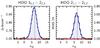 |
Fig. 2 Continuum subtracted spectra of the HDO 31,2 − 22,1 (225 GHz) and 21,1 − 21,2 (241 GHz) lines toward IRAS2A. The parental cloud velocity is shown by the dotted line (vlsr = 7 km s-1) and the Gaussian fits (blue) to the HDO lines are plotted along with the RMS (red). |
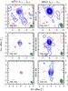 |
Fig. 3 Integrated intensity maps for the HDO 31,1 − 33,1 and H |
As noted in Jørgensen & van Dishoeck (2010a) and Persson et al. (2012, 2013) the HO lines are not found to be masing in these sources on the observed scales. This is in contrast to the 31,3 − 22,0 transition of the main isotopologue, HO, which is masing in many sources on single-dish scales (Cernicharo et al. 1994). The narrow widths of all detected HO and HDO lines presented here demonstrate that the lines do not originate from any outflow in these sources, where the lines have been observed to have broader widths (i.e., >5 km s-1Kristensen et al. 2010).
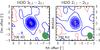 |
Fig. 4 Integrated intensity maps for the 31,2 − 22,1 (225 GHz) and 21,1 − 21,2 (241 GHz) transitions of HDO toward IRAS 2A, in the interval vline ± FWHM. The beam is shown in the lower right corner and the red crosses show the position of continuum peaks. Contours start at 39.6 mJy km s-1 (steps of 20σ), dashed contours represent negative values. |
Results from fits to the spectra and the (u,v)-plane.
Figure 3 shows the continuum subtracted intensity maps for all three sources and water lines. For IRAS 2A Fig. 4 shows the additional HDO line at 241.6 GHz together with the 225.9 GHz line. The intensity maps for each source are plotted on the same scale, i.e., the contour lines indicate the same intensities.
Circular Gaussian profiles were fitted to the emission of each line in the (u,v)-plane after integrating over channels corresponding to vlsr ± FWHM. Table 3 lists the FWHM of the 1D Gaussian fitted in the spectra, and size and intensity from fits in the (u,v)-plane of the integrated intensity for all the lines. The line widths roughly agree between the lines, being slightly wider in the HDO spectra (see Table 3).
4. Analysis
4.1. Spectra and maps
The spectra show similar characteristics for the observed sources and lines. The emission is compact and traces the warm water within 150 AU of the central sources. The integrated map for the IRAS 4A protobinary shows extended emission, partly aligned with the southern, blue-shifted outflow (Jørgensen et al. 2007). In contrast, the south-west outflow of IRAS 2A seen in HO is not detected in either of the two HDO lines. The ratio between the HDO line(s) and the HO line is similar for IRAS 2A and IRAS 4B, with HDO showing stronger emission than that of HO by a factor of four. In IRAS 4A-NW, the HDO 31,2 − 22,1 line is even brighter – about seven times stronger than the HO line. Methyl formate (CH3OCHO) is clearly seen toward IRAS 4A-NW and IRAS 4B in the 225 GHz spectra, while it is absent in the spectrum toward IRAS 2A. All lines toward IRAS 4B show very compact emission.
4.2. Column densities, excitation temperature and the HDO/H2O ratio
With two transitions of HDO observed toward IRAS 2A with different upper energy levels (Eu), a rough estimate of the excitation temperature (Tex) can be made. One issue is that the energy levels are quite close (167 vs. 95 K), which increases the uncertainty of the determined excitation temperature. Assuming that the HDO is optically thin and in LTE, and that the emission fills the beams uniformly, the excitation temperature for HDO in IRAS 2A is Tex = 124 ± 60 K, using a 20% flux calibration uncertainty. This excitation temperature reflects the bulk temperature of the medium averaged over the entire synthesized beam.
We can estimate the column density of HDO over the observed beam in all of the sources by assuming LTE with Tex = 124 K as determined for HDO in IRAS 2A, that the mission fills the beam and is optically thin. For IRAS 2A this is 11.9 ± 2.4 × 1015 cm-2, for IRAS 4A-NW it is 8.8 ± 1.8 × 1015 cm-2, and for IRAS 4B 1.5 ± 0.3 × 1015 cm-2. Assuming Tex = 124 K for the HO line as well gives column densities for the three sources consistent with the results of Persson et al. (2012), where Tex = 170 K was assumed.
With the column density of both HDO and HO, we deduce the water deuterium fractionation in all three protostars. For IRAS 2A the HDO/H2O ratio is then 7.4 ± 2.1 × 10⁻⁴, for IRAS 4A-NW it is 19.1 ± 5.4 × 10⁻⁴ and for IRAS 4B it is 5.9 ± 1.7 × 10⁻⁴. In the calculations a 16O/18O ratio of 560 was assumed, appropriate for the local interstellar medium (ISM; Wilson & Rood 1994). For IRAS 4B, the deduced HDO/H2O ratio agrees within the uncertainties with the upper limit derived by Jørgensen & van Dishoeck (2010b) using lower sensitivity SMA data.
To investigate the effects of different excitation temperatures, Fig. 5 shows the HDO/H2O ratio in IRAS 2A in the Tex range 40 − 400 K. As can be seen in the figure, the HDO/H2O ratio does not change significantly over this wide range of excitation temperatures: even if  is significantly different from Tex(HDO), the derived abundance ratios only vary by a factor of 3 from 5 − 15 × 10-4.
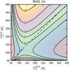 |
Fig. 5 Variation of the water deuterium fractionation (HDO/H2O) as a function of excitation temperature (40–400 K) for the observed water isotopologues. Contour values are × 10-4 and the dashed blue line shows where |

4.3. Radiative transfer modeling
To test our assumption of optically thin lines used to derive column densities in Sect. 4.2, full radiative transfer models of spherically symmetric envelopes have been run. These same type of models have been used to interpret the water and HDO emission lines observed by Herschel and single-dish ground based telescopes (Coutens et al. 2012, 2013). In these models, the molecular excitation is computed at each position in the envelope and subsequent line radiative transfer is performed. The interferometric data originate in the inner ~100 AU which is the scale on which the physical models are not well constrained. Previous observations have shown that flattened disk-like structures appear on scales ≲300 AU (Jørgensen et al. 2005; Chiang et al. 2012). Because of the lack of proper models, we adopt the spherically symmetric structure to assess the validity of the optically thin LTE approximation. Radiative transfer models were run for two cases: IRAS 16293-2422 and IRAS 2A.
The physical models start with a density structure which follows a power-law structure, as specified below for each of the sources. The dust temperature is then computed self-consistently as function of radius in the envelope for a given luminosity using the 1-D spherical dust continuum radiative transfer code TRANSPHERE (Dullemond et al. 2002). For the typical densities of the protostellar envelopes the gas is expected to be coupled to the dust and we thus assume that the gas and dust temperatures are identical (Jørgensen et al. 2002). The resulting temperature and density structure are then used as input to the Monte Carlo radiative transfer code RATRAN (Hogerheijde & van der Tak 2000). Since the line profiles do not show any complicated velocity structures the models only include a doppler broadening parameter (the “doppler-b parameter” 0.6 × FWHM). The outer radius is defined as where Tdust = 10 K or n = 104 cm-3, whichever comes first. HDO collisional rate coefficients of Faure et al. (2012) are used to calculate non-LTE population levels (LAMBDA database, Schöier et al. 2005). To produce the collisional rate coefficients for para-HO, the rates for HO from Daniel et al. (2011) for 5 < T < 1500 K were combined with the tabulated levels for para-HO from the JPL catalog (Pickett et al. 1998). The abundance of HDO or p-HO is then varied to obtain the best fit to the observed lines.
To determine the H2O abundance, the best-fit p-HO abundance has to be multiplied with the fraction of para to total water ratio (4, i.e. o/p = 3/1) and the 16O/18O ratio (560, Wilson & Rood 1994). The molecular abundance is assumed to follow a “jump” abundance profile (e.g., Schöier et al. 2004), with an inner and outer abundance that changes discontinuously at the point in the envelope where Tdust = 100 K, i.e., where water evaporates off the dust grains (Fraser et al. 2001). The radiative transfer model gives as output a model image cube with units Jy/pixel; this is then convolved with a beam corresponding to the observations and the integrated intensity is compared to those observed in Table 3 and Persson et al. (2013). To check where the emission in the relevant lines originates, the excitation is first solved for a model that covers the entire envelope, i.e. out to rout. Then an increasing number of cells are included in the ray-tracer, and the resulting integrated intensities are compared. This shows that the majority (>97%) of the emission in the observed lines comes from the region where T ≥ 100 K. To increase the numerical convergence, the envelope model for IRAS 2A was truncated at relatively small radii (6100 AU). The less dense and cold outer parts (R > 6100 AU) of the envelope does not contribute significantly to any absorption or emission of the observed lines.
For the IRAS 16293-2422 envelope, we adopt the same physical structure as developed by Crimier et al. (2010), which also allows us to compare our results to Coutens et al. (2012). In the original model a velocity field describing infall was used, here we set the turbulence doppler-b parameter to 1 km s-1 because we are only interested in fitting the total integrated intensity. Unless the lines are significantly optically thick, the adopted doppler-b parameter will only affect the line profile and not the total integrated intensity. The density structure of the envelope is described by Shu (1977) as 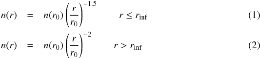 where rinf = 1280 AU, r0 = 76 AU and n(r0) = 2 × 108 cm-3 (the H2 number density at r0 where Tdust = 100 K). The dust opacity as a function of the frequency is set to a power-law emissivity model, i.e.,
 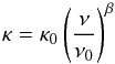 (3)where β = 1.8, κ = 15 cm2 g
 and ν0 = 1012 Hz. This dust opacity relation was adopted by Coutens et al. (2012) in order to fit the continuum observed with the Herschel-HIFI from 0.5 to 1 THz. The cold outer abundance at T < 100 K is fixed to Xout = 3 × 10-11 as found by Coutens et al. (2012) for both HDO and HO with respect to H2. Changing it within a reasonable interval (± 10 × Xout) does not change the derived warm inner abundances significantly.
The best fit to the 203 GHz HO line of IRAS 16293-2422 requires an inner abundance of Xin = 4.5 ± 0.9 × 10⁻⁸ (1.0 ± 0.2 × 10⁻⁴ for H2O), and for the HDO line at 225.9 GHz requires Xin = 11.0 ± 2.2 × 10⁻⁸. These abundances result in a HDO/H2O ratio of 10.9 ± 3.1 × 10⁻⁴. The models show that both HDO lines at 225.9 GHz and 241.6 GHz are marginally optically thick whereas the HO line is neither masing nor optically thick. The derived abundance ratio clearly agrees with the previously stated LTE, optically thin value of 9.2 ± 2.6 × 10⁻⁴ within the uncertainties (Persson et al. 2013). If the o/p ratio for the main collision partner (H2) is changed to 0, the HDO/H2O ratio goes down by 20%. For water, if an o/p ratio (H2O) of 1 and a 16O/18O ratio of 400 is assumed the HDO/H2O ratio increases by a factor of 2.8. This shows that the assumed o/p ratio of either H2O or H2 and the 16O/18O ratio can affect the resulting HDO/H2O ratio down by 20% and up by a factor of 2.8.
For IRAS 2A we have used the model described by Kristensen et al. (2012) and it extends from 35.9 AU (terminates where T > 250 K) to 17950 AU (but truncated at 6100 AU). The density profile is a single power-law, n(r) = n(r0) (r/r0)-1.7, where r0 = rin and n(r0) = 4.9 × 108 cm-3. The dust opacity is set to Table 1, Col. 5 in Ossenkopf & Henning (1994) (e.g., OH5 – dust grains with thin ice mantles) and the dust temperature is again computed self-consistently. The outer abundance is fixed to Xout = 3 × 10-11 for both HDO and HO, and as for IRAS 16293-2422, changing it within a reasonable interval (± 10 ×) does not change the derived abundances significantly. The best fit inner abundance for the HO line is Xin = 4.8±1.0 × 10⁻⁸ (1.1 ±0.2 × 10⁻⁴ for H2O), and Xin = 34.0 ± 6.8 × 10⁻⁸ for the HDO line at 225.9 GHz. This corresponds to a HDO/H2O ratio of 31.6 ± 8.9 × 10⁻⁴. While the HDO abundance derived from the 225 GHz line also fits the 241 GHz line within the uncertainties, the 143 GHz line observed by Taquet et al. (2013) is fit by a somewhat lower HDO abundance of Xin = 24.3 ± 4.9 giving a HDO/H2O ratio of 22.3 ± 6.4 × 10⁻⁴. All these HDO lines give a HDO/H2O ratio that is higher by a factor of 3 − 4 than the optically thin LTE value of 7.4 ± 2.1 × 10⁻⁴. This difference is largely due to the optical depth effects of the HDO lines.
The models for both IRAS 16293-2422 and IRAS 2A indicate that the HDO lines are marginally optically thick. This could indicate that the derived HDO column densities from the optically thin calculation (in Sect. 4.2) are slightly underestimated for all four sources. On the other hand, the HO line at 203.4 GHz is well constrained by LTE and is optically thin. Combined, this would imply an underestimate of the HDO/H2O ratio. However, the models show that this effect is minor, a factor of ~3 or less based on a comparison of the ratios derived from the radiative transfer models and the direct LTE estimates. The IRAS 16293-2422 example also shows that differential excitation effects of HDO versus HO can counteract the HDO optical depth effects.
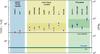 |
Fig. 6 Values of the HDO/H2O ratio, for different objects. For references, see Table A.1. Error bars for protostars reflect those obtained using the optically thin LTE approximation. |
5. Discussion and conclusions
All deduced HDO/H2O ratios are consistent with our previous low estimates for two deeply-embedded protostars (Persson et al. 2013; Jørgensen & van Dishoeck 2010b). The consistently low HDO/H2O ratios for all four sources suggests that the chemical evolution of water for these sources is similar.
Our high-resolution observations make it possible to focus on the compact warm gas. The sources show some extended emission in HDO and/or HO that would be included in any lower-resolution (single-dish) observations. Another key to our conclusions is that the observed lines are optically thin or at most marginally optically thick. Because of their higher Einstein A coefficients, the 31,2 − 30,3 lines of HO and HO observed with Herschel rapidly become optically thick, each at slightly different radii complicating the analysis (Visser et al. 2013). Unless the optical depth is properly treated, the HDO/H2O ratios deduced using Herschel data are likely to be overestimated. The ratio estimated for IRAS 2A by Visser et al. accounting for the optical thickness of the Herschel lines gives a HDO/H2O ratio of 1 × 10⁻³, in agreement with our estimates.
The recently deduced warm HDO/H2O ratios for IRAS 2A (3 × 10⁻³) and IRAS 4A (5 × 10⁻³) at the relevant densities (nH2 = 1 × 108 cm-3) by Taquet et al. (2013) are factors of 3–5 higher than our estimates. With a lower spectral (4 vs. 0.1 km s-1) and spatial (2′′ vs. 0.8′′) resolution than that of our HO data, the HDO observations used by Taquet et al. probe larger scales, thus are affected by extended emissions as observed in our observations at scales ≳500 AU (with higher HDO/H2O ratios as a probable result). Furthermore, the upper energy levels of the HDO and HO transitions differ significantly, Eu = 319 K for the HDO 42,2 − 42,3 transition vs. 204 K for the HO 31,3 − 22,0. The transitions could originate in slightly different regions depending on the source structure.
Coutens et al. (2013) used Herschel and several ground-based single dish telescopes to observe lines of HDO toward IRAS 4A and IRAS 4B. From 1D radiative transfer models and using the HO column density by Persson et al. (2012), they estimated HDO/H2O ratios in the inner warm regions of IRAS 4A (4.0 − 30.0 × 10⁻⁴) and IRAS 4B (1.0 − 37.0 ± 10-4). To reproduce the absorption seen in some of the spectral lines, a cold foreground absorbing layer is introduced. The results for the warm HDO/H2O ratio show a wide range but are consistent with our findings, namely that the ratio is similar for the two protostars, and that it is at most a few × 10-3.
The radiative transfer modeling highlights the uncertainties involved in the derivation of the HDO/H2O ratio. However, the ratios deduced with the optically thin LTE model-independent (i.e., not employing physical models and radiative transfer calculations to interpret the emission) method used in this paper and in Persson et al. (2013) is direct, and agrees with the full modeling within a factor of 3–4. Until the physical structure on small scales can be constrained, running full radiative transfer models can not yield a more accurate HDO/H2O ratio in the warm gas. However, spherically symmetric radiative transfer modeling can give indications on non-LTE effects and is a valid approximation for the outer envelope (e.g., Mottram et al. 2013). Furthermore, the modeling also confirms that the observed transitions of the water isotopologues are not masing in these environments.
The emerging picture of the water deuterium fractionation in warm inner regions of deeply-embedded low-mass protostars is therefore that of a consistent and relatively low ratio. While the protostars in this study are all located in the same star forming cloud, NGC 1333, IRAS 16293-2422 in Persson et al. (2013) is located in a different cloud, ρ Ophiuchus. Its similar HDO/H2O ratio indicates that a different birth environment does not necessarily imply a different ratio. To confirm this, HDO/H2O ratios determination toward more sources are needed.
Appendix A: Tables
HDO/H2O abundance ratios for different objects.
The infall timescales for the early, deeply-embedded stages are generally too short for any significant gas-phase chemical processing of water to take place in the warm >100 K gas before the material enters the disk (Schöier et al. 2002). Therefore the gaseous water observed here probably originates by sublimation of ice formed earlier in the evolution.
In Fig. 6 the deuterium fractionation of water for all four low-mass protostars (IRAS 2A, IRAS 4A-NW, IRAS 4B and IRAS 16293-2422) is presented together with those found in comets, Earth, ISM and protosolar values. The small differences in the amount of deuteration seen toward the inner regions of protostars and the comets in our solar system suggests that only small amounts of processing of water takes place between the deeply embedded stages and the formation of comets and planetesimals. If water was delivered to Earth by comets and small solar system bodies during the early evolution of the Sun, this would be the same water that was formed directly on the grain surface in the cold early stages of the formation of our Sun.
6. Summary and outlook
In this paper high-resolution interferometric observations of the HDO 31,2 − 22,1 line at 225.9 GHz toward three deeply embedded protostars have been presented. In addition, the HDO 21,1 − 21,2 line was observed toward one of the sources. With previous observations of HO (Persson et al. 2012), we deduce a model independent HDO/H2O ratio.
-
Observations of two HDO lines at high angu-lar resolution give an excitation temperature ofTex = 124 ± 60 K for IRAS 2A.
-
Assuming that the water emission is optically thin and is in LTE at Tex = 124 K for all three sources, we derive a HDO/H2O ratio of 7.4 ± 2.1 × 10⁻⁴ for IRAS 2A, 19.1 ± 5.4 × 10⁻⁴ for IRAS 4A-NW and 5.9 ± 1.7 × 10⁻⁴ for IRAS 4B.
-
The high-resolution interferometric observations give HDO/H2O ratios in a model independent way with an accuracy of a factor of 3–4, as confirmed by using non-LTE radiative transfer models. The fact that the observed lines have much lower optical depths than those observed with Herschel explains much of the early discrepancies in inferred values.
-
The HDO/H2O ratios deduced for these deeply-embedded protostars using interferometric observations are consistent from source to source. The ratios range from 5.9 to 19.1 × 10⁻⁴, close to those observed in solar system comets originating in the Oort cloud. The small difference between these reservoirs indicates little processing of material has taken place between the deeply-embedded, collapsing stage and the formation of comets/planetesimals.
Molecular data for the different lines, from JPL (Pickett et al. 1998) and CDMS (Müller et al. 2001).
D/H = 0.5 × HDO/H2O.
Vienna Standard Mean Ocean Water.
Spectra and maps are available through http://vilhelm.nu
Acknowledgments
We wish to thank the IRAM staff, in particular Arancha Castro-Carrizo and Chin Shin Chang, for their help with the observations and reduction of the data. We also appreciate discussions with Joe Mottram and Audrey Coutens on various aspects of water modeling. IRAM is supported by INSU/CNRS (France), MPG (Germany), and IGN (Spain). The research at Centre for Star and Planet Formation is supported by the Danish National Research Foundation and the University of Copenhagen’s programme of excellence. This research was also supported by a Junior Group Leader Fellowship from the Lundbeck Foundation to J.K.J. E.v.D. acknowledge the Netherlands Organization for Scientific Research (NWO) grant 614.001.008. E.v.D. and M.V.P. acknowledge EU FP7 grant 291141 CHEMPLAN. This work has benefited from research funding from the European Community’s sixth Framework Programme under RadioNet R113CT 2003 5058187.
References
- Biver, N., Bockelée-Morvan, D., Crovisier, J., et al. 2006, A&A, 449, 1255 [NASA ADS] [CrossRef] [EDP Sciences] [Google Scholar]
- Bockelée-Morvan, D., Gautier, D., Lis, D. C., et al. 1998, Icarus, 133, 147 [NASA ADS] [CrossRef] [Google Scholar]
- Bockelée-Morvan, D., Biver, N., Swinyard, B., et al. 2012, A&A, 544, L15 [NASA ADS] [CrossRef] [EDP Sciences] [Google Scholar]
- Cernicharo, J., Gonzalez-Alfonso, E., Alcolea, J., Bachiller, R., & John, D. 1994, ApJ, 432, L59 [NASA ADS] [CrossRef] [Google Scholar]
- Chiang, H.-F., Looney, L. W., & Tobin, J. J. 2012, ApJ, 756, 168 [NASA ADS] [CrossRef] [Google Scholar]
- Coutens, A., Vastel, C., Caux, E., et al. 2012, A&A, 539, A132 [NASA ADS] [CrossRef] [EDP Sciences] [Google Scholar]
- Coutens, A., Vastel, C., Cabrit, S., et al. 2013, A&A, 560, A39 [NASA ADS] [CrossRef] [EDP Sciences] [Google Scholar]
- Crimier, N., Ceccarelli, C., Maret, S., et al. 2010, A&A, 519, A65 [NASA ADS] [CrossRef] [EDP Sciences] [Google Scholar]
- Daniel, F., Dubernet, M.-L., & Grosjean, A. 2011, A&A, 536, A76 [NASA ADS] [CrossRef] [EDP Sciences] [Google Scholar]
- de Graauw, T., Helmich, F. P., Phillips, T. G., et al. 2010, A&A, 518, L6 [NASA ADS] [CrossRef] [EDP Sciences] [Google Scholar]
- de Laeter, J. R., Böhlke, J. K., De Bièvre, P., et al. 2003, Pure Appl. Chem., 75, 683 [CrossRef] [Google Scholar]
- Drake, M. J. 2005, Meteor. Planet. Sci., 40, 519 [Google Scholar]
- Dullemond, C. P., van Zadelhoff, G. J., & Natta, A. 2002, A&A, 389, 464 [NASA ADS] [CrossRef] [EDP Sciences] [Google Scholar]
- Duncan, M., Levison, H., & Dones, L. 2004, Comets II (Tucson: Univ. Arizona Press), 193 [Google Scholar]
- Eberhardt, P., Reber, M., Krankowsky, D., & Hodges, R. R. 1995, A&A, 302, 301 [NASA ADS] [Google Scholar]
- Enoch, M. L., Young, K. E., Glenn, J., et al. 2006, ApJ, 638, 293 [NASA ADS] [CrossRef] [Google Scholar]
- Faure, A., Wiesenfeld, L., Scribano, Y., & Ceccarelli, C. 2012, MNRAS, 420, 699 [NASA ADS] [CrossRef] [MathSciNet] [Google Scholar]
- Fraser, H. J., Collings, M. P., McCoustra, M. R. S., & Williams, D. A. 2001, MNRAS, 327, 1165 [NASA ADS] [CrossRef] [Google Scholar]
- Geiss, J., & Gloeckler, G. 1998, Space Sci. Rev., 84, 239 [NASA ADS] [CrossRef] [Google Scholar]
- Gibb, E. L., Bonev, B. P., Villanueva, G., et al. 2012, ApJ, 750, 102 [NASA ADS] [CrossRef] [Google Scholar]
- Hartogh, P., Lis, D. C., Bockelée-Morvan, D., et al. 2011, Nature, 478, 218 [NASA ADS] [CrossRef] [PubMed] [Google Scholar]
- Hersant, F., Gautier, D., & Huré, J.-M. 2001, ApJ, 554, 391 [NASA ADS] [CrossRef] [Google Scholar]
- Hogerheijde, M. R., & van der Tak, F. F. S. 2000, A&A, 362, 697 [NASA ADS] [Google Scholar]
- Hutsemékers, D., Manfroid, J., Jehin, E., Zucconi, J.-M., & Arpigny, C. 2008, A&A, 490, L31 [NASA ADS] [CrossRef] [EDP Sciences] [Google Scholar]
- Jehin, E., Manfroid, J., Hutsemékers, D., Arpigny, C., & Zucconi, J.-M. 2009, Earth Moon Planets, 105, 167 [NASA ADS] [CrossRef] [Google Scholar]
- Jennings, R. E., Cameron, D. H. M., Cudlip, W., & Hirst, C. J. 1987, MNRAS, 226, 461 [NASA ADS] [CrossRef] [Google Scholar]
- Jørgensen, J. K., & van Dishoeck, E. F. 2010a, ApJ, 710, L72 [NASA ADS] [CrossRef] [Google Scholar]
- Jørgensen, J. K., & van Dishoeck, E. F. 2010b, ApJ, 725, L172 [NASA ADS] [CrossRef] [Google Scholar]
- Jørgensen, J. K., Schöier, F. L., & van Dishoeck, E. F. 2002, A&A, 389, 908 [NASA ADS] [CrossRef] [EDP Sciences] [Google Scholar]
- Jørgensen, J. K., Bourke, T. L., Myers, P. C., et al. 2005, ApJ, 632, 973 [NASA ADS] [CrossRef] [Google Scholar]
- Jørgensen, J. K., Harvey, P. M., Evans, II, N. J., et al. 2006, ApJ, 645, 1246 [NASA ADS] [CrossRef] [Google Scholar]
- Jørgensen, J. K., Bourke, T. L., Myers, P. C., et al. 2007, ApJ, 659, 479 [NASA ADS] [CrossRef] [Google Scholar]
- Kavelaars, J. J., Mousis, O., Petit, J.-M., & Weaver, H. A. 2011, ApJ, 734, L30 [NASA ADS] [CrossRef] [Google Scholar]
- Kristensen, L. E., Visser, R., van Dishoeck, E. F., et al. 2010, A&A, 521, L30 [NASA ADS] [CrossRef] [EDP Sciences] [Google Scholar]
- Kristensen, L. E., van Dishoeck, E. F., Bergin, E. A., et al. 2012, A&A, 542, A8 [NASA ADS] [CrossRef] [EDP Sciences] [Google Scholar]
- Lellouch, E., Bézard, B., Fouchet, T., et al. 2001, A&A, 370, 610 [NASA ADS] [CrossRef] [EDP Sciences] [Google Scholar]
- Lis, D. C., Biver, N., Bockelée-Morvan, D., et al. 2013, ApJ, 774, L3 [NASA ADS] [CrossRef] [Google Scholar]
- Liu, F.-C., Parise, B., Kristensen, L., et al. 2011, A&A, 527, A19 [NASA ADS] [CrossRef] [EDP Sciences] [Google Scholar]
- Meier, R., Owen, T. C., Matthews, H. E., et al. 1998, Science, 279, 842 [NASA ADS] [CrossRef] [PubMed] [Google Scholar]
- Morbidelli, A., Chambers, J., Lunine, J. I., et al. 2000, Meteor. Planet. Sci., 35, 1309 [Google Scholar]
- Mottram, J. C., van Dishoeck, E. F., Schmalzl, M., et al. 2013, A&A, 558, A126 [NASA ADS] [CrossRef] [EDP Sciences] [Google Scholar]
- Müller, H. S. P., Thorwirth, S., Roth, D. A., & Winnewisser, G. 2001, A&A, 370, L49 [NASA ADS] [CrossRef] [EDP Sciences] [Google Scholar]
- Mumma, M. J., & Charnley, S. B. 2011, ARA&A, 49, 471 [NASA ADS] [CrossRef] [Google Scholar]
- Ossenkopf, V., & Henning, T. 1994, A&A, 291, 943 [NASA ADS] [Google Scholar]
- Parise, B., Simon, T., Caux, E., et al. 2003, A&A, 410, 897 [NASA ADS] [CrossRef] [EDP Sciences] [Google Scholar]
- Parise, B., Caux, E., Castets, A., et al. 2005, A&A, 431, 547 [NASA ADS] [CrossRef] [EDP Sciences] [Google Scholar]
- Persson, M. V., Jørgensen, J. K., & van Dishoeck, E. F. 2012, A&A, 541, A39 [NASA ADS] [CrossRef] [EDP Sciences] [Google Scholar]
- Persson, M. V., Jørgensen, J. K., & van Dishoeck, E. F. 2013, A&A, 549, L3 [NASA ADS] [CrossRef] [EDP Sciences] [Google Scholar]
- Pickett, H. M., Poynter, R. L., Cohen, E. A., et al. 1998, J. Quant. Spectr. Radiat. Transf., 60, 883 [Google Scholar]
- Prodanović, T., Steigman, G., & Fields, B. D. 2010, MNRAS, 406, 1108 [NASA ADS] [Google Scholar]
- Sandell, G., Aspin, C., Duncan, W. D., Russell, A. P. G., & Robson, E. I. 1991, ApJ, 376, L17 [NASA ADS] [CrossRef] [Google Scholar]
- Schöier, F. L., Jørgensen, J. K., van Dishoeck, E. F., & Blake, G. A. 2002, A&A, 390, 1001 [NASA ADS] [CrossRef] [EDP Sciences] [Google Scholar]
- Schöier, F. L., Jørgensen, J. K., van Dishoeck, E. F., & Blake, G. A. 2004, A&A, 418, 185 [NASA ADS] [CrossRef] [EDP Sciences] [Google Scholar]
- Schöier, F. L., van der Tak, F. F. S., van Dishoeck, E. F., & Black, J. H. 2005, A&A, 432, 369 [NASA ADS] [CrossRef] [EDP Sciences] [Google Scholar]
- Shu, F. H. 1977, ApJ, 214, 488 [NASA ADS] [CrossRef] [Google Scholar]
- Stark, R., Sandell, G., Beck, S. C., et al. 2004, ApJ, 608, 341 [NASA ADS] [CrossRef] [Google Scholar]
- Taquet, V., López-Sepulcre, A., Ceccarelli, C., et al. 2013, ApJ, 768, L29 [NASA ADS] [CrossRef] [Google Scholar]
- Villanueva, G. L., Mumma, M. J., Bonev, B. P., et al. 2009, ApJ, 690, L5 [NASA ADS] [CrossRef] [Google Scholar]
- Visser, R., Jørgensen, J. K., Kristensen, L. E., van Dishoeck, E. F., & Bergin, E. A. 2013, ApJ, 769, 19 [NASA ADS] [CrossRef] [Google Scholar]
- Wilson, T. L., & Rood, R. 1994, ARA&A, 32, 191 [NASA ADS] [CrossRef] [Google Scholar]
All Tables
Parameters of the continuum determined from elliptical Gaussian fits in the (u,v)-plane.
Molecular data for the different lines, from JPL (Pickett et al. 1998) and CDMS (Müller et al. 2001).
All Figures
|
Fig. 1 Continuum subtracted spectra of the H |
| In the text | |
|
Fig. 2 Continuum subtracted spectra of the HDO 31,2 − 22,1 (225 GHz) and 21,1 − 21,2 (241 GHz) lines toward IRAS2A. The parental cloud velocity is shown by the dotted line (vlsr = 7 km s-1) and the Gaussian fits (blue) to the HDO lines are plotted along with the RMS (red). |
| In the text | |
|
Fig. 3 Integrated intensity maps for the HDO 31,1 − 33,1 and H |
| In the text | |
|
Fig. 4 Integrated intensity maps for the 31,2 − 22,1 (225 GHz) and 21,1 − 21,2 (241 GHz) transitions of HDO toward IRAS 2A, in the interval vline ± FWHM. The beam is shown in the lower right corner and the red crosses show the position of continuum peaks. Contours start at 39.6 mJy km s-1 (steps of 20σ), dashed contours represent negative values. |
| In the text | |
|
Fig. 5 Variation of the water deuterium fractionation (HDO/H2O) as a function of excitation temperature (40–400 K) for the observed water isotopologues. Contour values are × 10-4 and the dashed blue line shows where |
| In the text | |
|
Fig. 6 Values of the HDO/H2O ratio, for different objects. For references, see Table A.1. Error bars for protostars reflect those obtained using the optically thin LTE approximation. |
| In the text | |
Current usage metrics show cumulative count of Article Views (full-text article views including HTML views, PDF and ePub downloads, according to the available data) and Abstracts Views on Vision4Press platform.
Data correspond to usage on the plateform after 2015. The current usage metrics is available 48-96 hours after online publication and is updated daily on week days.
Initial download of the metrics may take a while.