| Issue |
A&A
Volume 563, March 2014
|
|
|---|---|---|
| Article Number | A83 | |
| Number of page(s) | 24 | |
| Section | Stellar structure and evolution | |
| DOI | https://doi.org/10.1051/0004-6361/201322714 | |
| Published online | 14 March 2014 | |
Theoretical uncertainties of the Type Ia supernova rate⋆
1
Department of Astrophysics/IMAPPRadboud University Nijmegen,
PO Box 9010
6500 GL,
Nijmegen,
The Netherlands
e-mail:
This email address is being protected from spambots. You need JavaScript enabled to view it.
, This email address is being protected from spambots. You need JavaScript enabled to view it.
2
Argelander Institute for Astronomy, University of Bonn,
Auf dem Hügel 71,
53121
Bonn,
Germany
3
Anton Pannekoek Institute/GRAPPA, University of Amsterdam,
PO Box 94249,
1090 GE
Amsterdam, The
Netherlands
Received:
19
September
2013
Accepted:
12
January
2014
Abstract
It is thought that Type Ia supernovae (SNe Ia) are explosions of carbon-oxygen white dwarfs (CO WDs). Two main evolutionary channels are proposed for the WD to reach the critical density required for a thermonuclear explosion: the single degenerate (SD) scenario, in which a CO WD accretes from a non-degenerate companion, and the double degenerate (DD) scenario, in which two CO WDs merge. However, it remains difficult to reproduce the observed SN Ia rate with these two scenarios.
With a binary population synthesis code we study the main evolutionary channels that lead to SNe Ia and we calculate the SN Ia rates and the associated delay-time distributions. We find that the DD channel is the dominant formation channel for the longest delay times. The SD channel with helium-rich donors is the dominant channel at the shortest delay times. Our standard model rate is a factor of five lower than the observed rate in galaxy clusters.
We investigate the influence of ill-constrained aspects of single- and binary-star evolution and uncertain initial binary distributions on the rate of Type Ia SNe. These distributions, as well as uncertainties in both helium star evolution and common envelope evolution, have the greatest influence on our calculated rates. Inefficient common envelope evolution increases the relative number of SD explosions such that for αce = 0.2 they dominate the SN Ia rate. Our highest rate is a factor of three less than the galaxy-cluster SN Ia rate, but compatible with the rate determined in a field-galaxy dominated sample. If we assume unlimited accretion onto WDs, to maximize the number of SD explosions, our rate is compatible with the observed galaxy-cluster rate.
Key words: binaries: general / stars: evolution / supernovae: general
Tables 4 and 5, and appendices are available in electronic form at http://www.aanda.org
© ESO, 2014
1. Introduction
Type Ia supernovae (SNe Ia) are important astrophysical phenomena. On the one hand they drive galactic chemical evolution as the primary source of iron; on the other hand they are widely used as cosmological distance indicators (Phillips 1993; Riess et al. 1996, 1998; Perlmutter et al. 1999) because of their homogeneous light curves. Even so, the exact progenitor evolution remains uncertain. It is generally accepted that SNe Ia are thermonuclear explosions of carbon-oxygen white dwarfs (CO WDs; Nomoto 1982; Bloom et al. 2012). The explosion can be triggered when the CO WD reaches a critical density, which is reached when the mass approaches the Chandrasekhar mass (MCh = 1.4 M⊙, for non-rotating WDs). Single stars form a CO WD with a mass up to about 1.2 M⊙ (Weidemann 2000). To explain how the WD then reaches MCh two main channels are proposed: the single degenerate channel (SD; Whelan & Iben 1973; Nomoto 1982), in which the WD accretes material from a non-degenerate companion, and the double degenerate channel (DD; Webbink 1984; Iben & Tutukov 1984), in which two CO WDs merge.
Both channels cannot fully explain the observed properties of SNe Ia (Howell 2011). White dwarfs in the SD channel burn accreted material into carbon and oxygen, and therefore these systems should be observed as supersoft X-ray sources (SSXS, van den Heuvel et al. 1992), not enough of which are observed to explain the number of SNe Ia (Gilfanov & Bogdán 2010; Di Stefano 2010). However, Nielsen et al. (2013) argue that only a small amount of circumstellar mass loss is able to obscure these sources, making it difficult or even impossible for observers to detect them as SSXS. Moreover, during the supernova explosion some of the material from the donor star is expected to be mixed with the ejecta, which has never been conclusively observed (Leonard 2007; García-Senz et al. 2012). In some cases NaD absorption lines have been observed, which can be interpreted as circumstellar material from the donor star (Patat et al. 2007; Sternberg et al. 2011). Furthermore, the donor star is expected to survive the supernova explosion and to have a high space velocity. In the case of the 400 year old Tycho supernova remnant, we would expect to observe this surviving star. Nevertheless, no such object has been unambiguously identified (Ruiz-Lapuente et al. 2004; Kerzendorf et al. 2009; Schaefer & Pagnotta 2012). Some SNe and supernova remnants show evidence of interaction with circumstellar material which links them to the SD channel (Hamuy et al. 2003; Chiotellis et al. 2012; Dilday et al. 2012). However, a variation on the DD channel, in which the merger occurs during or shortly after the CE phase (Hamuy et al. 2003; Chevalier 2012; Soker et al. 2013), cannot be excluded as the progenitor channel for these SNe. Additionally, SN 2011fe, a SN Ia which exploded in a nearby galaxy, showed no evidence of interaction with circumstellar material at radio, X-ray, and optical wavelengths (e.g. Margutti et al. 2012; Chomiuk et al. 2012; Patat et al. 2013), and pre-explosion images exclude most types of donor stars of the SD channel (Li et al. 2011a).
These difficulties in reconciling the observational evidence with the predictions of the SD channel are avoided in the DD channel, but this channel has its own difficulties. In particular, Nomoto & Kondo (1991) show that the merger product evolves towards an accretion-induced collapse (AIC) rather than towards a normal SN Ia. Only recently, some studies indicate that the merger can lead to a SN Ia explosion under certain circumstances (Pakmor et al. 2010, 2011, 2013; Shen et al. 2013; Dan et al. 2014). Finally, binary population synthesis (BPS) studies show that neither channel reproduces the observed SN Ia rate (e.g. Ruiter et al. 2009; Mennekens et al. 2010; Toonen et al. 2012; Bours et al. 2013; Chen et al. 2012).
Using a BPS code, we investigate the progenitor evolution towards SNe Ia through the canonical Chandrasekhar mass channels: the SD and the DD channels. Our code makes it possible to study large stellar populations, to calculate SN Ia rates, and to compare these with the observed rate of SNe Ia. We analyse not only the different evolutionary channels, but also – in the case of the SD channel – determine general properties of the donor star at the moment of the explosion, and – in the case of the DD channel – of the merger product. The SN Ia rate has been studied by several groups through BPS; however, they used only a standard model without investigating in great detail the uncertainties in their model, or they investigated one uncertainty in binary evolution, such as the common envelope evolution (e.g. Yungelson & Livio 2000; Ruiter et al. 2009; Wang et al. 2009a, 2010; Mennekens et al. 2010; Toonen et al. 2012). We perform a study of the main parameters that play a role in the evolution towards Type Ia SNe which are ill-constrained. We study the effects on the predicted rate and on the progenitor evolution towards SNe Ia.
In Sect. 2, the BPS code and our model are described. In Sect. 3, the general progenitor evolution as it follows from our standard model is outlined. The resulting SN Ia rate is discussed in Sect. 4, while Sects. 5 and 6 treat the effects of varying the parameters on the progenitor evolution and the total rate. Finally, Sect. 7 discusses the validity of the Chandrasekhar model.
2. Binary population synthesis
We employ the rapid binary evolution code binary_c/nucsyn based on the work of Hurley et al. (2000, 2002) with updates described in Izzard et al. (2004, 2006, 2009) and below. We discuss the key assumptions of our model of single and binary star evolution. In Table 1 we list the assumptions in our standard model and give an overview of other possible assumptions, and the dependence of the theoretical SN Ia rate on them is discussed in Sects. 5 and 6. This code serves as the basis of our BPS calculations.
2.1. Single star evolution
Our single star models are analytic fits to detailed stellar models, described in Hurley et al. (2000), with updates of the thermally pulsating asymptotic giant branch (TP-AGB) which are fits to the models of Karakas et al. (2002), as described in Izzard et al. (2006). In the present study we adopt a metallicity Z of 0.02. We assume that only a CO WD can explode as a SN Ia based on the work of Nomoto & Kondo (1991) who found that an oxygen-neon (ONe) WD that reaches MCh undergoes AIC. Because CO WDs are formed only in low- and intermediate-mass binary systems, with a primary mass up to 10 M⊙, we limit our discussion to this mass range.
2.1.1. TP-AGB models
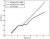 |
Fig. 1 Initial (Mi) versus final (Mf) mass of single stars that become CO WDs for different TP-AGB models (Sect. 2.1.1). The dotted line shows the results of the Hurley et al. (2000) models, the full line shows the results for the fits to the Karakas et al. (2002) models, and the dashed line shows our model. |
The evolution of the core, luminosity and radius of the TP-AGB star versus time are based on the models of Karakas et al. (2002), with the prescriptions described in Izzard et al. (2004, 2006). Because the core masses are determined without taking overshooting during previous evolution phases into account, a fit is made to take overshooting into consideration, based on the core masses calculated by Hurley et al. (2002) during the early-AGB (E-AGB). Up to and including the first thermal pulse, the core mass is calculated by the formulae described by Hurley et al. (2002). A smooth function is built in to guarantee a continuous transition of the radius between the E-AGB and the TP-AGB. Carbon-oxygen WDs form from stars with initial masses up to 6.2 M⊙, which correspond to a maximum CO-WD mass of about 1.15 M⊙ (Fig. 1).
2.1.2. Helium star evolution
In our model, if a hydrogen-rich star is stripped of its outer layers after the main sequence (MS) but before the TP-AGB, and the helium core is not degenerate, a helium star is formed. If the exposed core is degenerate, a He WD is made. The prescriptions that describe the evolution of naked helium stars are discussed in Hurley et al. (2000). However, because of its importance for the formation of Type Ia SNe we emphasize some details.
A distinction is made between three phases of helium star evolution: He-MS, the equivalent of the MS, when helium burns in the centre of the helium star; He-HG, the equivalent of the Hertzsprung gap (HG), when He-burning moves to a shell around the He-depleted core; and He-GB, the equivalent of the giant branch (GB), when the helium star has a deep convective envelope. If a non-degenerate helium core is exposed during the E-AGB, a star on the He-HG forms, otherwise a He-MS star forms.
A He-MS star becomes a He-WD when its mass is less than 0.32 M⊙, the minimum mass necessary to burn helium. The boundary between a helium star forming a CO WD or a ONe WD is determined by the mass of the star at the onset of the He-HG. The mass of the star on the He-HG should exceed 1.6 M⊙ in order to form a dense enough core to burn carbon and form an ONe-core, which is based on detailed models (carbon ignites off-centre when MCO,core ≳ 1.08 M⊙; Pols et al. 1998). The evolution of a He-HG star with M < 1.6 M⊙ leads to the formation of a CO WD with a mass greater than 1.2 M⊙ unless its envelope is lost by wind or binary mass transfer.
2.1.3. Wind mass loss
We adopt for both low- and intermediate-mass stars the prescription based on Reimers (1975) during the HG and beyond, multiplied
by a factor η, 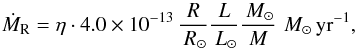 (1)where
M is the
mass, R and
L are the
radius and luminosity of the star, and η = 0.5 in our standard model (Table 1). During the TP-AGB we use the prescription based
on Vassiliadis & Wood (1993),
(1)where
M is the
mass, R and
L are the
radius and luminosity of the star, and η = 0.5 in our standard model (Table 1). During the TP-AGB we use the prescription based
on Vassiliadis & Wood (1993),
![Mathematical equation: \begin{equation} \label{eq::VW} \log \left(\!\frac{\dot{M}_{\rm VW}}{\Msun\,{\rm yr^{-1}}}\!\right) \!=\! -11.4 + 0.0125 \!\left(\!\frac{P_0}{d}\!-\!100 \max\left[\!\frac{M}{\Msun}\!-\!2.5,0.0 \right]\right),\,\, \end{equation}](/articles/aa/full_html/2014/03/aa22714-13/aa22714-13-eq41.png) (2)where
P0 is the Mira pulsation period in days
(d),
given by
(2)where
P0 is the Mira pulsation period in days
(d),
given by ![Mathematical equation: \begin{equation} \label{eq::P0} \log \left(\frac{P_0}{d}\right) = {\min}\left(3.3, -2.7 - 0.9 \log\left[\frac{M}{\Msun}\right] + 1.94 \log \left[\frac{R}{\Rsun}\right]\right)\cdot \end{equation}](/articles/aa/full_html/2014/03/aa22714-13/aa22714-13-eq44.png) (3)The wind is limited by
the steady superwind rate, ṀSW = 1.36 (L/ L⊙)M⊙ yr-1.
(3)The wind is limited by
the steady superwind rate, ṀSW = 1.36 (L/ L⊙)M⊙ yr-1.
In our model the wind of helium stars either follows the Reimers formula (Eq. (1)) or a prescription for Wolf-Rayet (WR)
stars (Hamann et al. 1995; Hamann & Koesterke 1998),
 (4)depending on which of
the two is stronger,
(4)depending on which of
the two is stronger,  (5)
(5)
2.2. Binary star evolution
Binary evolution can have a significant impact on the evolution of the individual stars in a binary system. Binary evolution is primarily determined by the initial semi-major axis (a) and the masses of the two stars. In the widest systems (a ≳ 105 R⊙) the stars do not interact, but evolve as though they were single. In closer systems (a ≲ 105 R⊙) interaction with the wind of the companion star can alter the evolution. In even closer systems (a ≲ 3 × 10³ R⊙) Roche-lobe overflow (RLOF) or common envelope (CE) evolution often has dramatic consequences for the further evolution of the two stars (Hurley et al. 2002). These different interactions are discussed below.
We assume the initial eccentricity (ei) is zero, based on the work of Hurley et al. (2002) who show that the evolution of close binary populations is almost independent of the initial eccentricity. We use the subscripts d and a for the donor and accreting star, respectively, and i for the initial characteristics of the star on the zero-age main sequence (ZAMS). We use the subscripts 1 and 2 for the initially more massive star, the primary, and the initially less massive star, the secondary, respectively. The mass ratio Ma/Md is denoted by Q, while the initial mass ratio qi is M2,i/M1,i.
2.2.1. Interaction with a stellar wind
Mass lost in the form of a stellar wind is accreted by the companion at a rate that
depends on the mass loss rate, the velocity of the wind and the distance to the
companion star. To describe this process and to calculate the rate Ṁa at which
material is accreted by the companion star, we use the Bondi-Hoyle prescription (Bondi & Hoyle 1944; Hurley et al. 2002), more specifically, ![Mathematical equation: \begin{equation} \label{eq::BH} \dot{M}_{\rm a} = \min \left(0.8 \dot{M}_{\rm d}, -1 \left[\frac{G M_{\rm a}}{v_{\rm d}^2}\right]^2 \frac{\alpha_{\rm BH}}{2a^2} \frac{1}{(1+v_{\rm rel}^2)^{3/2}} \dot{M}_{\rm d}\right), \end{equation}](/articles/aa/full_html/2014/03/aa22714-13/aa22714-13-eq61.png) (6)with
Ṁd the mass loss rate from the donor
star, e the
eccentricity, a the semi-major axis, vd the wind
velocity of the donor star which we assume equals 0.25 times the escape velocity as
proposed by Hurley et al. (2002), and
vrel = |vorb/vd |,
with vorb the orbital velocity. The
Bondi-Hoyle accretion efficiency parameter, αBH, is set to 3/2 in our standard
model (Table 1). When both stars lose mass
through a wind they are treated independently; no interaction of the two winds is
assumed.
(6)with
Ṁd the mass loss rate from the donor
star, e the
eccentricity, a the semi-major axis, vd the wind
velocity of the donor star which we assume equals 0.25 times the escape velocity as
proposed by Hurley et al. (2002), and
vrel = |vorb/vd |,
with vorb the orbital velocity. The
Bondi-Hoyle accretion efficiency parameter, αBH, is set to 3/2 in our standard
model (Table 1). When both stars lose mass
through a wind they are treated independently; no interaction of the two winds is
assumed.
Some observed RS CVn systems show that the less evolved star is the more massive of the
binary before RLOF occurs; therefore, it has been suggested that wind mass loss is
tidally enhanced by a close companion (Tout &
Eggleton 1988). It is uncertain whether this phenomenon occurs for other types
of binaries. To approximate this effect the following formula is implemented (Tout & Eggleton 1988), ![Mathematical equation: \begin{equation} \label{TE88} \dot{M} = \dot{M}_{\rm R} \left( 1+ B_{\rm wind} \cdot \max \left[\frac{1}{2},\frac{R}{R_{\rm L}} \right]^6 \right), \end{equation}](/articles/aa/full_html/2014/03/aa22714-13/aa22714-13-eq67.png) (7)where
RL is the Roche radius of the star
(Eggleton 1983). In our standard model
Bwind = 0 (Table 1).
(7)where
RL is the Roche radius of the star
(Eggleton 1983). In our standard model
Bwind = 0 (Table 1).
2.2.2. Stability of RLOF
Critical mass ratio Qcrit for stable RLOF for different types of donor stars, in the case of a non-degenerate and a degenerate accretor.
Whether or not mass transfer is stable depends on 1) the reaction of the donor, because a star with a convective envelope responds differently to mass loss than a star with a radiative envelope; 2) the evolution of the orbit, which itself depends on the accretion efficiency (β = Ṁa/Ṁd) and the mass ratio Q = Ma/Md; and 3) the reaction of the accreting star. In our model the criterion to determine whether mass transfer is stable is given by a critical mass ratio Qcrit, which depends on the types of donor and accreting stars (Table 2). During RLOF the mass ratio Q of the binary system is compared with Qcrit: if Q < Qcrit mass transfer is dynamically unstable and a CE phase follows, otherwise RLOF is stable. In Table 2 we list the values of the critical mass ratios for the different phases of the evolution of a star during accretion onto either a non-degenerate or a degenerate star.
Roche-lobe overflow from a MS donor is generally stable because a radiative MS star shrinks in reaction to mass loss. When material is transferred to a MS companion, RLOF is stable only for certain mass ratios because a radiative accreting star expands and can fill its own Roche lobe. If the mass ratio is less than 0.625 the system evolves into a contact system and we assume the two MS stars merge (de Mink et al. 2007). The stability criteria for the other types of donor stars transferring mass to a non-degenerate companion are calculated according to Hurley et al. (2002).
To calculate Qcrit of WDs, we assume that during RLOF almost no material is accreted onto the WD, β = 0.01, and the specific angular momentum of the ejected material is that of the orbit of the accreting star (Hachisu et al. 1996). Because of the low accretion efficiencies of WDs (Appendix B), the critical mass ratio for stable mass transfer decreases. Our adopted critical mass ratios for mass transfer from non-degenerate donor stars onto a WD are calculated with the formulae from Soberman et al. (1997; Chiotellis, priv. comm.).
2.2.3. Common envelope evolution
If the donor star is an evolved star and the mass ratio of the Roche-lobe overflowing
system is less than its critical value (Table 2),
the system evolves into a CE. We use the α-prescription to describe this complex phase
(Webbink 1984), in which the binding energy
(Ebind) of the CE is compared with the
orbital energy (Eorb) of the system to calculate the
amount the orbit should shrink in order to lose the envelope of the donor star. More
specifically, αce is defined by  (8)where the subscripts
i and f correspond to the states before and after the CE phase, respectively, and where
(8)where the subscripts
i and f correspond to the states before and after the CE phase, respectively, and where
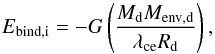 (9)and Md,
Menv,d, and
Rd are the mass, the envelope mass, and
the radius of the donor, respectively, and G is the gravitational constant.
(9)and Md,
Menv,d, and
Rd are the mass, the envelope mass, and
the radius of the donor, respectively, and G is the gravitational constant.
The CE efficiency parameter, αce, describes how efficiently the energy is transferred from the orbit to the envelope. Its value is expected to be between 0 and 1, although it could be larger than 1 if another energy source is available, such as nuclear energy. In our standard model we take αce = 1 (see Table 1). The parameter λce depends on the relative mass distribution of the envelope, and is not straightforward to define (Ivanova 2011). According to Ivanova (2011) its value is close to 1 for low-mass red giants and therefore in many studies is taken as such. In our model λce is variable and is dependent on the type of star, its mass, and its luminosity. We use a prescription based on Dewi & Tauris (2000; our Appendix A), which gives a value of λce between 0.25 and 0.75 for HG stars, between 1.0 and 2.0 for GB and AGB stars, and λce = 0.5 for helium stars. Because of the short timescale of the CE phase (e.g. Passy et al. 2012), we assume in our standard model that no mass is accreted by the companion star (Table 1).
Additional energy sources, e.g. the ionization energy of the envelope, can boost the envelope loss. The extended envelope can become cool enough that recombination of hydrogen occurs in the outer layers. In our model the fraction of the ionization energy that is used is expressed by λion, which is between 0 and 1 (Appendix A). In our standard model this effect is not considered and λion = 0 (Table 1).
2.2.4. Stable RLOF
When mass transfer is stable (Q > Qcrit,
Table 2), the mass transfer rate is calculated as
a function of the ratio of the stellar radius of the donor Rd and the
Roche radius RL (based on Whyte & Eggleton 1980), ![Mathematical equation: \begin{equation} \label{H02} \dot{M} = f \cdot 3.0\times 10^{-6} \, \left(\log\left[\frac{R_{\rm d}}{R_{\rm L}}\right]\right)^3 \, \left({\min}\left[\frac{M_{\rm d}}{\Msun},5.0\right]\right)^2 \Msun \, \rm yr^{-1}. \end{equation}](/articles/aa/full_html/2014/03/aa22714-13/aa22714-13-eq91.png) (10)The last,
mass-dependent factor in the equation is defined by Hurley et al. (2002) for stability reasons. In Hurley et al. (2002) the dimensionless factor f is 1; however, this
underestimates the rate when mass transfer proceeds on the thermal timescale. In our
model f is
not a constant, but depends on the stability of mass transfer. If f is large, the radius
stays close to the Roche radius and mass transfer is self-regulating. However, in our
model numerical instabilities arise when log Rd/RL ≲ 10-3
and the envelope of the donor star is small. Therefore, a function is defined that
forces the radius to follow the Roche radius more closely during thermal-timescale mass
transfer (f
= 1000) and more loosely during nuclear timescale mass transfer (f = 1). A smooth
transition is implemented between the two extreme values of f. To test the stability
of the function that calculates the mass transfer rate, a binary grid was run with
binary_c/nucsyn consisting of 503 binary systems with initial
primary masses between 2 M⊙ and 10 M⊙, secondary
masses between 0.5 M⊙ and 10 M⊙, and
initial separations between 3 R⊙ and 104 R⊙. The mass
transfer rates of systems evolving through the SD channel with a hydrogen-rich donor
were used to optimize this function for computational stability. The resulting function
is given by
(10)The last,
mass-dependent factor in the equation is defined by Hurley et al. (2002) for stability reasons. In Hurley et al. (2002) the dimensionless factor f is 1; however, this
underestimates the rate when mass transfer proceeds on the thermal timescale. In our
model f is
not a constant, but depends on the stability of mass transfer. If f is large, the radius
stays close to the Roche radius and mass transfer is self-regulating. However, in our
model numerical instabilities arise when log Rd/RL ≲ 10-3
and the envelope of the donor star is small. Therefore, a function is defined that
forces the radius to follow the Roche radius more closely during thermal-timescale mass
transfer (f
= 1000) and more loosely during nuclear timescale mass transfer (f = 1). A smooth
transition is implemented between the two extreme values of f. To test the stability
of the function that calculates the mass transfer rate, a binary grid was run with
binary_c/nucsyn consisting of 503 binary systems with initial
primary masses between 2 M⊙ and 10 M⊙, secondary
masses between 0.5 M⊙ and 10 M⊙, and
initial separations between 3 R⊙ and 104 R⊙. The mass
transfer rates of systems evolving through the SD channel with a hydrogen-rich donor
were used to optimize this function for computational stability. The resulting function
is given by ![Mathematical equation: \begin{equation} \label{calcF} f = \begin{cases} 1000 & Q < 1 \text{ and} \\ \displaystyle \max \left(1, \frac{1000}{Q}\cdot \exp\left[-\frac{1}{2} \left\{\frac{\ln Q}{0.15}\right\}^2 \right]\right) & Q > 1. \\ \end{cases} \end{equation}](/articles/aa/full_html/2014/03/aa22714-13/aa22714-13-eq98.png) (11)Because
mass transfer is dynamically stable, the mass transfer rate is capped at the thermal
timescale mass transfer rate ṀKH, given by
(11)Because
mass transfer is dynamically stable, the mass transfer rate is capped at the thermal
timescale mass transfer rate ṀKH, given by 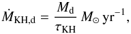 (12)with τKH the
thermal timescale of the donor star,
(12)with τKH the
thermal timescale of the donor star, 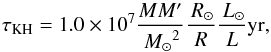 (13)and
M′ is the mass of the star, if the star
is on the MS or the He-MS; otherwise, M′ is the envelope mass of the star.
(13)and
M′ is the mass of the star, if the star
is on the MS or the He-MS; otherwise, M′ is the envelope mass of the star.
In order to test the mass transfer rate calculated with our BPS code, as a next step a set of binary systems and their mass transfer rates were calculated with our BPS code and with a detailed binary stellar evolution code (STARS, Eggleton 1971, 2006; Pols et al. 1995; Glebbeek et al. 2008) and compared. We simulated a grid with primary masses that varied between 2 M⊙ and 6 M⊙, secondary masses that varied between 0.7 M⊙ and 3.5 M⊙, and orbital periods varied between 2 days and 4 days (to check binary systems with both MS and HG donors). We also simulated a more massive binary system of 12 M⊙ and 7 M⊙ at orbital periods of 3.5 days and 4 days. We find that the resulting maximum mass transfer rate computed with the BPS code is larger by about a factor of three (for MS donors) and a factor of five (for HG donors) than the maximum from the detailed stellar evolution code, with the duration of thermal timescale mass transfer correspondingly shorter. Additionally, we find similar durations of the entire mass transfer phase calculated with both codes.
In addition, the accretor adjusts its structure to the accreted mass. If the mass
transfer rate is higher than the thermal timescale rate of the accretor, the accreting
star is brought out of thermal equilibrium, resulting in expansion and additional mass
loss from the accretor. Consequently, during RLOF the fraction of transferred material
that is accreted is not taken to be constant, but depends on the thermal timescale of
the accretor. For moderately unevolved stars (stars on the MS, HG or helium stars) the
accretion efficiency β is calculated in our model as 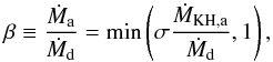 (14)where
σ is a
parameter for which we assume a value of 10 in our standard model (as in Hurley et al. 2002). Moreover, in the case of
accretion onto a MS or He-MS star, rejuvenation is assumed (Hurley et al. 2002). The internal structure of the star is changed
and new fuel is mixed into the burning region, which results in a star that appears
younger. If the accretor is an evolved star on the GB or AGB, mass transfer is assumed
to be conservative (β = 1) because a convective star shrinks as a
reaction to mass gain. Accretion onto a WD is a special situation because of its
degeneracy and this will be discussed separately below.
(14)where
σ is a
parameter for which we assume a value of 10 in our standard model (as in Hurley et al. 2002). Moreover, in the case of
accretion onto a MS or He-MS star, rejuvenation is assumed (Hurley et al. 2002). The internal structure of the star is changed
and new fuel is mixed into the burning region, which results in a star that appears
younger. If the accretor is an evolved star on the GB or AGB, mass transfer is assumed
to be conservative (β = 1) because a convective star shrinks as a
reaction to mass gain. Accretion onto a WD is a special situation because of its
degeneracy and this will be discussed separately below.
When material is lost from the system it removes angular momentum. Angular momentum
loss is described with a parameter γ that expresses the specific angular momentum of
the lost material in terms of the average specific orbital angular momentum as follows:
 (15)In our standard model
we assume that during stable RLOF material is lost by isotropic re-emission, removing
the specific orbital angular momentum of the accretor (γ = Md/Ma;
Table 1).
(15)In our standard model
we assume that during stable RLOF material is lost by isotropic re-emission, removing
the specific orbital angular momentum of the accretor (γ = Md/Ma;
Table 1).
2.2.5. Stable RLOF onto a WD
Because a WD is degenerate, it burns accreted material stably only over a small range of mass transfer rates which corresponds to approximately 10-7 M⊙/yr when hydrogen-rich material is accreted and 10-6 M⊙/yr when helium-rich material is accreted (Nomoto 1982). If the mass transfer rate is too low, the material is not burnt immediately and a layer of material is deposited on the surface. This layer burns unstably, resulting in novae. If the mass transfer rate is too high, the WD cannot burn all the accreted material. According to Nomoto (1982) the accreted material forms an envelope around the WD and becomes similar to a red giant with a degenerate core and, generally, a CE subsequently forms. Hachisu et al. (1996) propose that the burning material on top of the WD drives a wind that blows away the rest of the accreted material. The accreted material burns at the rate of stable burning, but contact is avoided and mass transfer remains stable. We take this possibility into account (for a description see Appendix B). The material ejected through the wind from the WD removes specific angular momentum from the WD (γ = Md/Ma). The above also holds for WDs accreting through a wind, but the material transferred to the WD is based on the Bondi-Hoyle accretion efficiency (Eq. (6)).
2.3. Binary population synthesis
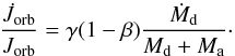
We simulate NM1,i × NM2,i × Nai
binary systems in log M1,i−log M2,i−log ai space, with M1,i and M2,i the initial masses
of the primary and secondary stars and ai the initial semi-major axis of the
binary systems. The volume of each cell in the parameter space is δM1,i δM2,i δai.
To compute the SN rate each system is assigned a weight Ψ according to the initial distributions of
binary parameters. We normalize the SN rate to the total mass of the stars in our grid,
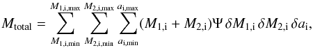 (16)where
-
M1,i,min = 0.1 M⊙ and M1,i,max = 80 M⊙,
-
M2,i,min = 0.01 M⊙ (Kouwenhoven et al. 2007) and M2,i,max = M1,i,
-
ai,min = 5 R⊙ and ai,max = 5 × 10⁶ R⊙ (Kouwenhoven et al. 2007), and
-
Ψ is the initial distribution of M1,i, M2,i, and ai.
We assume that Ψ is
separable, namely  (17)where
-
ψ(M1,i) is the initial distribution of primary masses from Kroupa et al. (1993, Table 1,
-
φ(M2,i) is the initial secondary masses distribution, which we assume is flat in M2,i/M1,i, and
-
χ(ai) is the initial distribution of semi-major axes, which we assume is flat in log ai (Öpik 1924; Kouwenhoven et al. 2007).
We calculate the delay-time distribution (DTD), which is the SN rate as a function of
time per unit mass of stars formed in a starburst at t = 0, 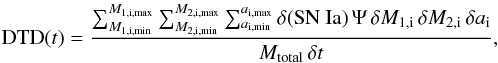 (18)where
δ(SN Ia) = 1 if the binary system leads to a SN Ia
event during a time interval t to t + δt, otherwise δ(SN Ia) = 0. We assume
all stars are formed in binaries, which is an overestimate of the binary fraction, because
for low-mass stars the observed fraction of systems in binaries is less than 50% (Lada 2006). However, in intermediate-mass stars, Kouwenhoven et al. (2007) find a best fit with 100%
binaries and Duchêne & Kraus (2013)
conclude that different surveys are consistent with a multiplicity higher than 50%.
Additionally, Kobulnicky & Fryer (2007) and
Sana et al. (2012) find that more than 70% of
massive stars are in binary systems.
(18)where
δ(SN Ia) = 1 if the binary system leads to a SN Ia
event during a time interval t to t + δt, otherwise δ(SN Ia) = 0. We assume
all stars are formed in binaries, which is an overestimate of the binary fraction, because
for low-mass stars the observed fraction of systems in binaries is less than 50% (Lada 2006). However, in intermediate-mass stars, Kouwenhoven et al. (2007) find a best fit with 100%
binaries and Duchêne & Kraus (2013)
conclude that different surveys are consistent with a multiplicity higher than 50%.
Additionally, Kobulnicky & Fryer (2007) and
Sana et al. (2012) find that more than 70% of
massive stars are in binary systems.
The results of Sect. 3 are calculated by simulating a grid with M1,i between 2.5 M⊙ and 9 M⊙, M2,i between 1 M⊙ and M1, and ai between 5 R⊙ and 5 × 10³ R⊙, with NM1,i = NM2,i = Nai = N = 150.
3. Binary progenitor evolution
In this section we discuss the general progenitor evolution of the different SN Ia channels, SD and DD, and their contribution according to our standard model (Sect. 2). We describe binary evolution in terms of the number of stable or unstable phases of RLOF and the stellar types at the onset of mass transfer. This illustrates the influence of different aspects of binary evolution and initial binary distributions (Sects. 5 and 6). In the following sections the mass ratio q is M2/M1, where the suffixes 1 and 2 denote the initially more and less massive star, respectively.
3.1. Double degenerate channel
 |
Fig. 2 Initial separation (ai) versus initial mass of the primary star (Mi, left) and versus initial mass ratio (M2,i/M1,i, right) of systems that form SNe Ia through the DD channel in our standard model (Sect. 2). Number density (greyscale) represents the number of systems normalized to the total number of systems forming a SN Ia through the DD channel. Lines show the minimum separation (assuming q = 1) for which the primary fills its Roche lobe at a certain stage of evolution, as indicated. Symbols A–F indicate differences in the evolutionary stage when the primary fills its Roche lobe and in the number of CE phases necessary to evolve to a SN Ia: A = HG, no CE; B = HG, 1 CE (the difference between B1 and B2 is based on which of the two stars first forms a WD); C = GB, 1 CE; D = E-AGB, 1 CE; E = TP-AGB, 1 CE; F = TP-AGB, 2 CEs. |
The double degenerate channel (DD) needs two CO WDs, with a combined mass greater than MCh in a short enough orbit (a ≲ 4 R⊙), to merge within a Hubble time. Consequently, the rate of this channel depends on the number of systems that, after phases of stable RLOF and/or CE evolution, are in such a short orbit. The results of Pakmor et al. (2010, 2011) indicate that the violent merger of two CO WDs only results in an explosion for a limited range of mass ratios. In combination with possible mass loss during the merger, this restriction can reduce the SN Ia rate from the DD channel by about a factor of five (Chen et al. 2012). However, in this work we do not impose a restriction on the mass ratio of the two CO WDs.
Multiple formation channels can form close double WD systems (Mennekens et al. 2010; Toonen et al. 2012). Mennekens et al. (2010) distinguish between the common envelope channel, which needs two consecutive CE phases, and the Roche-lobe overflow channel, in which a phase of stable Roche-lobe overflow is followed by a CE phase. Additionally, Toonen et al. (2012) discuss the formation reversal channel where the secondary forms a WD first. Figure 2 shows the distribution of systems that evolve towards SNe Ia according to the DD channel in terms of their initial separation ai, initial primary mass M1,i, and initial mass ratio qi. We distinguish six main regions: two lower regions A and B, with ai/R⊙ ≲ 300, in which the primary fills its Roche lobe during the HG; two intermediate regions C and D, with 300 ≲ ai/R⊙ ≲ 1000, in which the primary fills its Roche lobe during the GB or E-AGB; and two upper regions E and F, with ai/R⊙ ≳ 1000, in which one or more CE phases are needed and the primary fills its Roche lobe during the TP-AGB.
Close systems: regions A and B.
If the initial separation is shorter than about 300 R⊙ the primary first fills its Roche lobe on the HG when the star has a radiative envelope. The first phase of mass transfer is thus stable and a CE is avoided.
The separation and the mass of the secondary determine whether the second phase of mass transfer, from the secondary, is stable. The separation determines both the moment the secondary fills its Roche lobe and the stellar type of the secondary at RLOF. The initially closest systems with the least massive secondaries avoid a CE and two CO WDs form in a short orbit without any CE phase (region A), while the wider systems experience a CE phase when the secondary fills its Roche lobe (region B).
Region A consists of systems that avoid a CE phase during their entire evolution. The range of initial mass ratios that make SNe Ia is strongly restricted (Fig. 2), because systems with initial mass ratios larger than 0.46 form double WD systems in an orbit too wide to merge in a Hubble time. Because of this restriction, only 0.7% of the systems that become a SN Ia via the DD channel follow this evolutionary channel. However, when RLOF is followed with a detailed stellar evolution code, some of these systems with a mass ratio smaller than 0.46 that contain an accreting MS-star are expected to form a contact system (de Mink et al. 2007) which eventually merges before the formation of two CO WDs.
Region B represents the most common evolutionary channel and corresponds to the Roche-lobe overflow channel (Mennekens et al. 2010; Toonen et al. 2012). In this region the primary starts mass transfer during the HG and a CE phase occurs when the secondary fills its Roche lobe. This channel accounts for 84% of SNe Ia formed through the DD channel in our model, a similar fraction to Mennekens et al. (2010). Binary systems with initial masses lower than 2.9 M⊙ do not form a merger product with a combined mass greater than 1.4 M⊙, while systems with primary masses higher than 8.2 M⊙ form an ONe WD. Binary systems with mass ratios lower than 0.25 have an unstable first mass transfer phase and merge.
In region B we distinguish between regions B1 and B2, based on which of the two stars becomes a WD first. In general, the initially more massive star is expected to form the first WD of the binary system (region B1). However, sometimes the evolution of the secondary catches up with the primary because of previous binary interaction and becomes a WD first (region B2), which is the formation reversal channel (Toonen et al. 2012). Region B2 contains 49% of the systems forming region B (41% of all DD systems).
The systems of region B2 have primary masses between 2.9 M⊙ and 5 M⊙ and mass ratios between 0.67 and 1. When a hydrogen-rich star loses its envelope before the TP-AGB it becomes a helium star before evolving into a WD (Sect. 2.1). In this case the resulting helium stars have a mass between 0.5 M⊙ and 0.85 M⊙. The time it takes for these low-mass helium stars to become a WD is long (between about 40 Myr and 160 Myr) which gives the secondary, which has increased in mass, time to evolve and fill its Roche lobe. It becomes the most massive helium star of the binary system after the subsequent CE phase. The short orbit after the CE phase allows the secondary to fill its Roche lobe again and evolve into the first WD of the binary system. Afterwards, the primary fills its Roche lobe for the second time and becomes the second WD of the binary system. The range of primary masses that make SNe Ia is restricted because the lifetime of the corresponding helium star has to be long enough for the secondary to evolve. This restriction originates from the necessity for the secondary to fill its Roche lobe before the primary becomes a WD.
Systems with initial separations in the gap between region B and regions C and D do not form a double WD system. The primary fills its Roche lobe at the end of the HG or on the GB, which leads to a CE phase in which the two stars merge.
Wide systems that undergo one CE phase: regions C, D, and E.
In systems with separations longer than about 300 R⊙, the primary fills its Roche lobe after the HG while having a convective envelope which results in a CE phase. The primary becomes a WD immediately (region E) or after subsequent evolution as a helium star (regions C and D). Afterwards, the secondary fills its Roche lobe. In regions C, D, and E mass transfer from the secondary is stable, permitting accretion onto the initial WD. However, the WD cannot reach MCh before the secondary loses its entire envelope and the binary becomes a short-period double WD system. This imposes a restriction on the range of initial mass ratios that make SNe Ia, which determines the separation after the phase of stable RLOF, because the orbit should be short enough when the secondary becomes a WD. This channel produces 12.8% of DD progenitors (1.9% in region C, 6.3% in region D, and 4.6% in region E). The difference between the three regions is the stellar type of the primaries at the onset of mass transfer: in region C the primary is on the GB, in region D on the E-AGB, and in region E on the TP-AGB (Fig. 2).
The ranges of the initial masses of the three evolutionary channels are defined by the necessity for both stars to become a CO WD (upper limit on the masses) and form a massive enough merger (lower limit on the masses). In some systems with a mass ratio close to one (qi ≳ 0.93) the secondary is already evolved at the moment the primary fills its Roche lobe and during the CE phase both envelopes are lost. The secondary still fills its Roche lobe after the primary becomes a WD, but as a helium star, namely on the He-HG.
The systems with initial separation in the gap between regions D and E do not form double WD systems. These systems survive the first CE phase and form a helium star with a non-evolved companion. However, because of the longer initial separation, the helium star fills its Roche lobe again as a He-giant. This leads to a second CE phase, during which the two stars merge.
Wide systems that undergo two CE phases: region F.
When the initial separation is longer than about 1000 R⊙ the first mass transfer phase starts when the primary is on the TP-AGB. This leads to unstable mass transfer and therefore a CE phase, during which the separation decreases. The primary becomes a CO WD immediately. Subsequently, the secondary fills its Roche lobe which also results in unstable mass transfer. This evolutionary channel is similar to the common envelope channel discussed in Mennekens et al. (2010) and Toonen et al. (2012). This channel produces 2.4% of the DD systems. These systems have the first phase of mass transfer during the TP-AGB (Fig. 2), however this evolutionary channel also occurs when mass transfer starts during the E-AGB. Nevertheless, the systems that start RLOF during the E-AGB and have two consecutive CE phases generally merge before the formation of a double WD system and only account for 0.1% of all DD systems.
In systems with longer initial separations (a ≳ 2500 R⊙), both stars do not fill their Roche lobe, and therefore do not form double WD systems in a short orbit (Fig. 2).
3.2. Single degenerate channel
The single degenerate channel needs a CO WD and a non-degenerate companion that provides enough mass to the WD at a high enough rate. We distinguish between hydrogen-rich and helium-rich companions.
3.2.1. SD with hydrogen-rich donor (SDH)
A hydrogen-rich companion can be in any evolutionary stage between the MS and the AGB. The stability criterion for mass transfer (Table 2) and the rate at which mass is transferred determine which donor stars transfer enough material to the WD to make SNe Ia. Evolved stars (GB or AGB) have a convective envelope, which results in a smaller critical mass ratio for stable mass transfer compared to non-evolved stars (MS or HG) with a radiative envelope (Table 2). Consequently, donors on the MS can be more massive than evolved donors without the system evolving into a CE. In addition, the mass transfer rate determines the amount of material that is accreted by the WD. Ideally, the mass transfer rate is about 10-7 M⊙ yr-1 (Nomoto 1982, Sect. 2). Mass transfer is generally faster from GB donors than from MS donors with the same mass. Consequently, compared to MS stars, stars on the GB can be initially less massive to donate enough mass to a CO WD to grow to MCh (Fig. 3).
The contours in Fig. 3 show the results of a simulation with our BPS code in log M1,i−log M2,i−log ai space as discussed in Sect. 2.3 with N = 125, in which one of two stars is a WD at t = 0 and the other is on the ZAMS. The initial masses range between 0.7 M⊙ and 1.15 M⊙ for the WD and between 0.7 M⊙ and 6 M⊙ for the companion MS star, the separation is varied between the minimum separation for a MS star to fill its Roche lobe and 103 R⊙ and we assume ei = 0. The figure shows the possible ranges in donor mass and separation for which WDs with a mass of 0.8, 1.0, or 1.15 M⊙ can grow to MCh.
In Fig. 3 three main regions are distinguished with MWD < 1.15 M⊙. The donor stars in the region with log a/ R⊙ ≲ 1.2 and 1.5 ≲ Md/ M⊙ ≲ 5.2 start transferring mass to the WD during the MS, the donor stars in the region with 1.0 ≲ log a/ R⊙ ≲ 1.5 and 2.4 ≲ Md/ M⊙ ≲ 3.0 during the HG, and those in the region with 2.0 ≲ log a/ R⊙ ≲ 2.5 and 1.15 ≲ Md/ M⊙ ≲ 1.4 during the GB. For future reference we name these channels the WD+MS, WD+HG, and WD+RG channels, respectively, as in Mennekens et al. (2010).
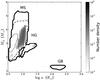 |
Fig. 3 Donor mass (Md) versus separation (a) at the moment of formation of the CO WD of the systems producing SNe Ia through the SDH channel, for different CO WD masses: 1.15 M⊙ (solid line), 1.0 M⊙ (dash-dotted line), and 0.8 M⊙ (dotted line). The greyscale shows how these regions are populated in our standard model. Labels indicate the different stellar types of donors stars. |
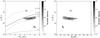 |
Fig. 4 As Fig. 2 for systems that form SNe Ia through the SDH channel. Symbols AH, BH, and CH indicate groups which are distinguished based on the evolutionary stage when the primary fills its Roche lobe and the number of CE phases necessary to evolve to a SN Ia: AH = HG, no CE; BH = end of HG/GB, 1 CE; CH = TP-AGB, 1 CE. |
Figure 3 in this article can be compared with Fig. 3 of Han & Podsiadlowski (2004), which was calculated with a detailed binary stellar evolution code and which discussed the WD+MS channel. Like Han & Podsiadlowski (2004) we find that SNe Ia can originate from accreting WDs with donor masses between 1.5 M⊙ and 3.5 M⊙, but in addition we find systems with donor masses greater than 3.5 M⊙, which they find to become dynamically unstable and hence do not become SNe Ia. This arises because of a different treatment of the stability of RLOF between the two codes. For the WD+RG channel we compare our results with Fig. 2 of Wang & Han (2010) who find donor masses down to 0.6 M⊙. However, these systems do not become a SN Ia within a Hubble time and therefore are not shown in our Fig. 3.
The greyscale in Fig. 3 depicts the number density at WD formation of the systems evolving through the SDH channel with our standard model. To understand why our standard model does not form WD+MS systems over the entire mass and separation range shown in Fig. 3, a closer look at the distribution of the initial characteristics of the systems which evolve into a SN Ia through the SDH channel is necessary (Fig. 4). In this figure three regions are distinguished: systems with short (AH), intermediate (BH), and long initial separations (CH).
Close systems: region A H .
Systems with initial separation between 20 R⊙ and 70 R⊙ have the first phase of RLOF during the HG, which is stable. Subsequently a WD forms in a short orbit because of the initially low mass ratio. Afterwards the systems evolve through the WD+MS channel (Fig. 3). Only 1% of the SDH systems evolve through this channel, because of the small initial mass ratios involved and the possibility of the formation of a contact system because of the reaction of the secondary during accretion (cf. region A of the DD channel, Sect. 3.1).
Wide systems: regions B H and C H .
The most common evolutionary channel (99%) of the SDH channel is through a CE after which the WD is in a short orbit with an unevolved companion. The systems of region BH follow the WD+MS channel, while the systems of region CH follow the WD+HG channel or the WD+RG channel.
In region BH, systems have initial separations longer than 300 R⊙ and the primary fills its Roche lobe at the end of the HG or the onset of the GB. After the CE phase a helium star forms, which subsequently overflows its Roche lobe stably and evolves into a WD. The secondary fills its Roche lobe during the MS and follows the WD+MS channel. This evolutionary channel is followed by 99% of the SDH systems, with 21% starting RLOF at the end of the HG and 78% during the GB. A star with an initial mass between 5.7 M⊙ and 8.2 M⊙ evolves into a CO WD with a mass between 0.8 M⊙ and 0.95 M⊙ when stripped of its hydrogen envelope at the end of the HG or during the GB. This explains why the greyscale in Fig. 3 is limited in the mass range of the donors. Binary systems with initial separations longer than 400 R⊙ after a CE phase, as well as systems with initial separations shorter than 200 R⊙ after a phase of stable mass transfer, form a WD binary system that is too wide to go through the WD+MS channel (Fig. 3).
In region CH, systems have initial separations longer than 1000 R⊙ and the primary fills its Roche lobe during the TP-AGB and forms a CO WD immediately. After the CE phase the secondary fills its Roche lobe as an evolved star on the HG or GB; 0.3% of the SDH systems follow this evolutionary channel. The number of systems going through this evolutionary channel is limited because only systems with CO WDs with initial masses larger than about 1.1 M⊙ can grow to MCh with an evolved donor star. Additionally, the WD+RG channel is almost non-existent as binary systems with a massive WD (≳1.0 M⊙) and a low-mass MS star (≲1.5 M⊙) rarely form with separations between 100 R⊙ and 300 R⊙ with the assumed CE efficiency and therefore cannot contribute to the WD+RG channel.
Systems with initial separations longer than about 3000 R⊙ do not experience RLOF and therefore do not become a SN Ia. However, these systems still interact in the form of a stellar wind. Nevertheless, in our standard model wind mass transfer is insufficient for a CO WD to grow to MCh (Sect. 2.2.1).
3.2.2. SD with helium-rich donors (SDHe)
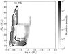 |
Fig. 5 As Fig. 3 for systems at the formation of the WD and He-MS binary that produce SNe Ia through the SDHe channel. |
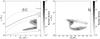 |
Fig. 6 As Fig. 2 for systems that form SNe Ia through the SDHe channel. Symbols AHe, BHe, and CHe indicate groups that are distinguished based on the evolutionary stage when the primary fills its Roche lobe, the number of CE phases necessary to evolve to a SN Ia, and the type of donor star transferring mass to the CO WD: AHe = HG, no CE, with He-MS donors; BHe = HG, 1 CE, with He-HG donors; CHe = TP-AGB, 1 CE. |
Helium-rich donors must be massive enough (M ≳ 1 M⊙) to transfer enough material to the WD to make a SN Ia. Consequently, their H-rich progenitor stars must be massive enough initially (at least 4 M⊙). The initial helium star can be non-evolved (He-MS) or evolved (He-HG or He-GB). Figure 5 shows the results of a simulation similar to that of Sect. 3.2.1, with one of the stars at t = 0 a WD and the other star on the zero-age He-MS. The ranges of both masses, the separation, and the resolution are equal to those discussed in Sect. 3.2.1.
Figure 5 depicts the helium donor masses versus the separation of the systems with an initial WD mass ≤1.15 M⊙ that become SNe Ia. Two regions are distinguished. The left region with log a/ R⊙ ≲ 0.2 and 0.9 ≲ Md/ M⊙ ≲ 4.5 shows systems that start RLOF to the WD during the He-MS. The middle region with 0.0 ≲ log a/ R⊙ ≲ 0.85 and 1.05 ≲ Md/ M⊙ ≲ 1.5 shows donor stars that start RLOF to the WD during the He-HG; He-GB donors do not form SNe Ia when the initial WD mass is less than 1.15 M⊙ because the evolutionary timescale of these stars is too short to transfer much material to a WD.
Helium MS stars more massive than 1.6 M⊙ explode as core collapse SNe (CC SNe) if they evolve as single stars (Pols et al. 1998). This potentially allows some binary systems to produce both a SN Ia, from the CO WD, and subsequently a core collapse SN from the remaining He star. However, He-MS donors with these masses transfer much material to the WD and have masses lower than 1.6 M⊙ when the CO WD reaches MCh. In our model the structure of He-MS adapts during RLOF and the star evolves further as though it started its evolution with this new mass. These initially massive helium stars then become a WD instead of exploding as a CC SN. However, if the He-MS star does not adapt to its new mass during RLOF, we find that one binary system in our grid produces both a SN Ia and a CC SN.
Our Fig. 5 should be compared with Fig. 8 in Wang et al. (2009b), which depicts the systems evolving through the WD+He-MS and WD+He-HG channel calculated with a detailed binary stellar evolution code. Both figures indicate that helium donors with masses down to about 0.9 M⊙ transfer at least 0.25 M⊙ to a 1.15 M⊙ WD. However, we find that helium stars more massive than 3 M⊙ can also transfer this amount stably to a WD, while Wang et al. (2009b) find that RLOF is dynamically unstable in these binary systems because of differences in the stability criteria of RLOF between the two codes. In addition, they find slightly higher donor masses in the WD+He-HG channel, which in our model do not transfer enough material to the WD companion.
The greyscale of Fig. 5 represents the number density of the systems at the formation of a WD and helium star binary for the SDHe channel. Below we describe the different progenitor evolutionary channels, distinguishing between systems with initially short separations that have He-MS donors (AHe) or He-HG donors (BHe) and systems with initially long separations (CHe). These different groups can be distinguished in Fig. 6.
Close systems: regions A He and B He .
Systems with initial separations between 25 R⊙ and 300 R⊙ have primaries that fill their Roche lobe during the HG when they have radiative envelopes which results in stable mass transfer. After mass transfer a helium star is formed which becomes a WD without interaction or after a phase of stable RLOF. Afterwards a CO WD and a MS star, which has increased in mass, remain. Because of the great difference in mass between the two stars a CE phase follows when the secondary fills its Roche lobe during the HG or beyond, but before the TP-AGB. Subsequently a CO WD and helium star in a short orbit remain. When the secondary fills its Roche lobe for the second time the WD increases in mass and reaches MCh.
The main difference between regions AHe and BHe is the moment the companion star fills its Roche lobe as a helium star, i.e. during the He-MS at the shortest separations (region AHe) and during the He-HG at the longest separations (region BHe).
The initial primary mass and mass ratio of both groups are determined by the need to form a CO WD (upper mass and mass ratio limit) and a massive enough merger product (lower mass and mass ratio limit). The lower primary mass boundary of region AHe is lower than that of region BHe because less massive WDs can grow to MCh with He-MS donors (Fig. 5).
Of the SDHe systems, 48% follow the evolutionary channel of region AHe. The range of initial separations is limited by the small range of radii of He-MS stars (Fig. 5). Systems with shorter separations than 25 R⊙ merge during the CE phase before the formation of a helium star, while in systems with longer separations than about 55 R⊙ the helium stars fill their Roche lobes after the He-MS. The evolutionary channel of region BHe is followed by 48% of the SDHe systems. Systems with separations shorter than about 55 R⊙ have the helium star filling its Roche lobe during the He-MS, while initially longer separations than 300 R⊙ evolve into a CE phase when the primary fills its Roche lobe.
In our standard model some binary systems form WDs with masses greater than 1.15 M⊙ because the core of the helium star forming the WD grows beyond 1.15 M⊙ (see Sect. 2.1.2). This results in higher mass donors that can transfer enough material to these massive WDs to reach MCh than indicated by the solid line in Fig. 5. This explains why our model produces He-star donors with masses larger than 1.5 M⊙ at a ≈ 10 R⊙ outside the solid contour in Fig. 5.
Wide systems: region C He .
SN Ia progenitor systems with initial separations longer than 1000 R⊙ have an initial mass ratio close to one (q ≳ 0.91). The primary fills its Roche lobe during the TP-AGB which results in a CE and a CO WD is formed. Moreover, because the two stars stars have comparable masses, generally the secondary is also an evolved star at the moment of RLOF. Afterwards, a CO WD and a helium star in a short orbit are formed. However, some systems fill their Roche lobes during the GB shortly after the primary, which results in a second CE phase after which the secondary becomes a helium star. In both cases, the helium star (He-MS or He-HG) fills its Roche lobe afterwards, which increases the mass of the WD to MCh. Only a small range of mass ratios follow this channel because smaller companion masses evolve into helium donor stars that are not massive enough. This channel accounts for only 4% of systems in the SDHe channel.
4. Comparison with observations
In this section we compare the rate of the previously discussed channels and the sum of the three channels, the overall SN Ia rate, with observations. The delay-time distribution represents the SN Ia rate per unit mass of stars formed as a function of time, assuming a starburst at t = 0. The DTD allows us to investigate the validity of the different progenitor models, by providing a direct comparison with observations.
In early studies the observed DTD was described by a two-component model (Scannapieco & Bildsten 2005; Mannucci et al. 2006). The first component accounts for
the prompt SNe Ia before 300 Myr, while the second component accounts for the delayed SNe Ia
which have delay times longer than 300 Myr. More recent observations show that the DTD is
best described by a continuous power-law function with an index of −1 (Totani
et al. 2008; Maoz et al. 2010, 2011; Maoz &
Mannucci 2012; Graur et al. 2011; Graur & Maoz 2013), more specifically (Maoz & Mannucci 2012) 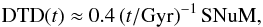 (19)where SNuM is the
supernova rate per 100 yr per 1010 M⊙. According to Totani et al. (2008) this relation supports the DD channel and arises
from a combination of the initial separation distribution of the systems
(
(19)where SNuM is the
supernova rate per 100 yr per 1010 M⊙. According to Totani et al. (2008) this relation supports the DD channel and arises
from a combination of the initial separation distribution of the systems
( )
and the timescale of gravitational radiation (τGWR ∝ a4).
Some groups find a different slope, for example Pritchet et
al. (2008) find a t−0.5 ± 0.2 relation. To compare
our models to observed DTDs, we use Eq. (18).
)
and the timescale of gravitational radiation (τGWR ∝ a4).
Some groups find a different slope, for example Pritchet et
al. (2008) find a t−0.5 ± 0.2 relation. To compare
our models to observed DTDs, we use Eq. (18).
We also compare the integrated SN Ia rate, i.e. the number of SNe Ia (NSN) per unit of stellar mass formed in stars over the history of the Universe. Maoz & Mannucci (2012) conclude that the number of SNe Ia between 35 Myr and the Hubble time (13.7 Gyr) is consistent with 2 × 10⁻³ M⊙-1. However, more recent determinations of the observed SN Ia rate show that the integrated rate may be lower than previously assumed. Different groups find an integrated rate between 0.33 × 10⁻³ and 2.9 × 10⁻³ M⊙-1 (Maoz et al. 2011, 2012; Graur et al. 2011; Graur & Maoz 2013; Perrett et al. 2012). Maoz et al. (2012) suggest that the divergence may be explained by enhancement of SNe Ia in galaxy cluster environments at long delay times compared to field environments. The lower limit on these observations, however, is found by Graur & Maoz (2013) by applying a t-1 relation for the DTD and they did not consider the previously discussed uncertainties of the slope. Because their integrated rate is based on SNe Ia with long delay times, a steeper power law results in a higher integrated rate. To compare with our models, we use an integrated rate of 2.3 × 10⁻³ M⊙-1 as found by Maoz et al. (2011). Below we describe the rate of the different channels and the overall SN Ia rate resulting from our standard model (Figs. 7 and 8).
4.1. Double degenerate rate
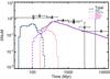 |
Fig. 7 Delay-time distribution of the different channels with our standard model (Sect. 2): the SDHe channel (blue dash-dotted line), the SDH channel (red dotted line), the DD channel (purple dashed line), and the overall SN Ia rate (black thin full line), which is the sum of the three channels. The rate is presented in units of SNuM which is the SN Ia rate per 100 yr per 1010 M⊙ in stars. Data points represent the observed DTD from Totani et al. (2008, triangles) and Maoz et al. (2011, squares). |
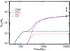 |
Fig. 8 Number of SNe Ia (NSN) per unit mass versus time, with our standard model (Sect. 2). Line styles have the same meaning as in Fig. 7. Data points show the integrated rate (over a Hubble time) determined by Maoz et al. (2011, diamond), Maoz et al. (2012, square), and Graur & Maoz (2013, triangle). |
In our standard model, the DD channel begins after about 100 Myr and dominates the SN Ia rate from about 200 Myr up to a Hubble time (Fig. 7, dashed line). The delay time of the DD channel can be described by a continuous power-law function from about 400 Myr. However, because the DTD is the combination of different evolutionary channels, it does not exactly follow a t-1 relationship, but rather a t-1.3 relation. Region B (Fig. 2), i.e. the Roche-lobe overflow channel, contributes from about 100 Myr up to a Hubble time and is always the dominant evolutionary channel. Regions D and E, which form double WD systems after one CE phase followed by a phase of stable RLOF, also contribute with a few percent to the DTD after about 200 Myr up to a Hubble time. The rate following from our standard model for long delay times (averaged between 300 Myr and a Hubble time) is 0.031 SNuM and peaks at about 400 Myr. The integrated rate is 4.3 × 10⁻⁴ M⊙-1.
Another observable prediction of the DD channel is the mass of the merger product, which can be up to 2.4 M⊙. A merger product of 2.4 M⊙ can lead to an overluminous SN Ia if all its mass is burnt (e.g. Yoon & Langer 2005). If only 1.4 M⊙ of the mass is burnt it can leave about 1 M⊙ of unburnt carbon and oxygen which can be observed in the spectrum. Figure 9 shows that of all double WD systems with a combined mass higher than MCh, 50% have a combined mass larger than 1.65 M⊙. However, only about 3% with have a combined mass greater than 2 M⊙ would be classified as super-Chandrasekhar because of the current limitations in defining the total WD mass of the progenitor systems leading to observed SNe Ia (e.g. Howell et al. 2006).
4.2. Single degenerate rate
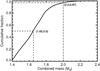 |
Fig. 9 Cumulative distribution of the combined mass of the two CO WDs merging within a Hubble time for WD mergers having a combined mass greater than 1.4 M⊙ in our standard model. The lines indicate specific masses and cumulative fractions (Sect. 4.1). |
The delay time of the SD channel depends on the evolutionary timescale of the secondary, the donor star to the exploding CO WD. The range of initial masses of the different types of donor stars (Sect. 3.2) is apparent in their respective DTDs. The helium-rich donors are initially the most massive and therefore the resulting SNe Ia occur earlier than the SNe Ia formed through the SDH channel (Fig. 7, dash-dotted line and dotted line).
The SD channel with helium rich donors contributes between about 45 Myr and about 200 Myr. This short time frame arises because only initially massive secondary stars, which have a helium core greater than 1 M⊙, can transfer enough material to the CO WD as a helium star. Assuming a starburst the average rate between 40 Myr and 200 Myr is 0.092 SNuM and the integrated rate is 1.5 × 10⁻⁵ M⊙-1.
In the SD channel with hydrogen rich donors we distinguish between non-evolved and evolved donors. The shortest delay times occur for MS and HG donors, while the more delayed SNe Ia originate from GB donors. Type Ia SNe formed through the WD+MS channel occur from about 170 Myr until 500 Myr, the WD+HG channel contributes at about 450 Myr. The WD+RG channel contributes from about 4000 Myr, but is not significant and cannot be distinguished in the DTD.
4.3. Overall SN Ia rate
The sum of the three channels results in a DTD best described by a broken power-law, slightly increasing before 100 Myr, a dip between 200 Myr and 400 Myr, and t-1.3 relation afterwards (Fig. 7). The dominant formation channel of prompt SNe Ia is the SDHe channel, while the dominating channel of longer delay times is the DD channel. Assuming a starburst, the rate between 40 Myr and 100 Myr is on average 0.14 SNuM and is dominated by the SDHe channel. The average rate between 100 Myr and 400 Myr is 0.22 SNuM with approximately equal contributions from the SD and DD channels. At longer delay times, the DD channel dominates (Table 5 and Fig. 7). The integrated rate is 4.8 × 10⁻⁴ M⊙-1, with about 95% of the SNe Ia formed through the DD channel, and is approximately a factor of five lower than the Maoz et al. (2011) rate, but compatible with the lowest estimates for the SN Ia rate (Graur & Maoz 2013, Fig. 8).
Additionally, we find that 2.4% of intermediate-mass stars with a primary mass between 3 M⊙ and 8 M⊙ explode as SNe Ia. This is compatible with the lower limit, expressed as η, given by Maoz (2008) based on several observational estimates; more specifically they find that η ≈ 2−40%. However, Maoz (2008) suggests that η = 15% is consistent with all the different observational estimates discussed in the paper, which is about a factor of six higher than our results.
The SN Ia rate versus the rate of core collapse SNe (CC SNe) is another observable prediction. We find that NSNIa/NSNCC = 0.07−0.14, where the upper limit is determined by assuming that all primaries with a mass between 8 M⊙ and 25 M⊙ explode as CC SNs and the lower limit is determined by assuming that both primaries and secondaries with a primary mass between 8 M⊙ and 25 M⊙ explode as CC SNe. Mannucci et al. (2005) determine this ratio based on star forming galaxies and find NSNIa/NSNCC = 0.35 ± 0.08. Cappellaro et al. (1999) estimate a lower ratio of 0.28 ± 0.07, as do Li et al. (2011b), who find that NSNIa/NSNCC = 0.220 ± 0.067 and 0.248 ± 0.071 for the prompt and the delayed SN Ia components, respectively. On the other hand, de Plaa et al. (2007) find a higher ratio of 0.79 ± 0.15 based on X-ray observation of the hot gas in clusters of galaxies. Our ratio is between two and four times smaller than the ratio found by Cappellaro et al. (1999), and more than a factor of five lower than the ratio estimated by de Plaa et al. (2007).
5. Uncertainties in binary evolution
The theoretical rate and delay-time distribution of Type Ia SNe depends on many aspects of binary evolution, such as CE evolution, angular momentum loss, and the stability criterion of Roche-lobe overflowing stars, some of which are not well constrained. In order to test the dependence of the progenitor evolution and the rate on the assumptions we performed 35 additional simulations with our BPS code, labelled A to R, each letter indicating a variation in a parameter, and numerical subscripts indicating different values for important parameters. We only discuss the most important parameters, while in Tables 4 and 5 we give an overview of our results. Variations of the initial distributions of binary parameters are discussed in Sect. 6. The results discussed in this section and the next are calculated with a resolution of N = 100 (Sect. 2.3), except for the simulation of conservative RLOF (N = 150) and the simulation with γwind = 2 (N = 125), in which the ranges of both initial masses and separation are longer than in our standard model. For comparison we list in Tables 4 and 5 the results of our standard model with N = 150 to show that choosing a higher resolution only has a small effect.
5.1. Common envelope evolution
In both the SD and DD channels the prescription of the CE phase is crucial because almost all progenitor systems go through at least one CE phase. This phase is modelled by comparing the binding energy of the envelope and the orbital energy, the αce-prescription, which is parametrized by the parameters αce and λce (Sect. 2.2.3). Below we describe the effect of varying both parameters separately.
5.1.1. Common envelope efficiency
The CE efficiency αce plays a crucial role in the progenitor evolution. We vary αce between 0.2 and 10 (models A1 to A4). Different groups determine a CE efficiency smaller than 1 after fitting the αce-prescription to a population of observed post-CE binaries (Zorotovic et al. 2010; De Marco et al. 2011; Davis et al. 2012). Zorotovic et al. (2010) found that only a CE efficiency between 0.2 and 0.3 reproduces their entire observed sample. A CE efficiency of 10 is an extreme assumption to demonstrate the effect of an efficient extra energy source during the CE phase.
SD channel.
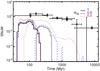 |
Fig. 10 DTD of the SD channel for the assumptions discussed in Sect. 2 and with variable CE efficiency αce: 1 (black full line), 0.5 (blue dashed line), and 0.2 (red dotted line). The thick lines show the SDHe channel, while the thin lines show SDH channel. Data points have the same meaning as in Fig. 7. |
In our models with lower common-envelope efficiencies than our standard model (models A1 and A2, with αce = 0.2 and 0.5, respectively), systems with initially longer separations than in our standard model survive a CE phase and contribute to the SDH channel, more specifically to the WD+MS channel and the WD+HG channel. Stars that are stripped of their envelopes at a later stage of their evolution have more massive cores and form more massive WDs. Generally, the mass range of accreting WDs increases with decreasing CE efficiency. More specifically, in the WD+MS channel for αce = 1 the initial mass of the CO WD ranges between 0.8 M⊙ and 0.95 M⊙, while for αce = 0.2 (model A1) the initial mass of the CO WD ranges between 0.8 M⊙ and 1.15 M⊙, with an associated increase in the integrated rate (Fig. 3 and Table 4), from 0.9 × 10⁻⁵ M⊙-1 when αce equals 1, to 9.0 × 10⁻⁵ M⊙-1 when αce equals 0.2.
Additionally, the DTD changes significantly (Fig. 10 and Table 5). As the mass range of the donor stars of the WD+MS and WD+HG channels is enlarged, the rate of the SD channel increases and contributes for a longer time. The rate of the WD+RG channel does not increase in models A1 and A2 because binary systems formed after RLOF with massive CO WDs (MWD > 1.0 M⊙) and low-mass MS stars (M < 2.0 M⊙) have separations shorter than 30 R⊙ and therefore do not contribute to the WD+RG channel (Fig. 3).
In the case of higher CE efficiencies we find the opposite (models A3 and A4): the WD+MS and WD+HG channels decrease and the WD+RG channel increases (Table 4). In model A4 (αce = 10) the DTD of the SDH channel mainly consists of a delayed component from SNe Ia formed through the WD+RG channel. Likewise, the integrated rate of the SDHe channel increases in models A1 and A2, but only by a factor of two to three because of the already large mass range of CO WDs formed when αce equals 1.
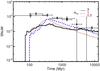 |
Fig. 11 DTD of the DD channel for our standard model (Sect. 2) and with variable CE efficiency αce: 3 (black full line), 1 (blue dashed line), and 0.5 (red dotted line). Data points have the same meaning as in Fig. 7. |
DD channel.
Two effects play a role when changing the CE efficiency (Fig. 11 and Tables 4 and 5). The first effect is the selective evolution towards a formation reversal (Table 4, region B2). In the formation reversal channel, the CE phase preceding the formation of the second helium star brings two helium stars together in a short orbit. If αce = 1, the more massive helium star fills its Roche lobe when it is an evolved helium star. If the orbit is too wide after the CE phase and the helium star does not fill its Roche lobe, the subsequently formed WDs do not merge within a Hubble time. At small αce the more massive helium star fills its Roche lobe at an earlier evolutionary stage, during the He-MS, and the double WD system does not form a massive enough merger product. This evolutionary channel completely disappears at low CE efficiency (e.g. αce = 0.2, model A1) and almost completely for high CE efficiencies (e.g. αce = 10, model A4). It appears that αce = 1 is an optimal value for this formation path (Table 4).
The second effect is that the lower and upper separation boundaries for regions B to F would change to longer separations in the models with lower CE efficiencies compared to our standard model. However, systems with longer separations are less common and in some regions the movement of the upper boundary is limited, such as in region F. In region F, the initially widest binary systems in which both stars fill their Roche lobe already form SNe Ia when αce = 1. These two implications decrease the DD rate assuming lower CE efficiencies (Table 4).
On the other hand, if the CE efficiency is very high (e.g. αce = 10, Table 4), the orbital energy does not decrease much during a CE phase and fewer double WD systems evolve into a short enough orbit to merge within a Hubble time. Consequently, the rate of the DD channel decreases for very high CE efficiencies. Regions C to E almost disappear when αce = 10. The rate of region F increases when αce = 3 and 10, but these SNe Ia originate from binary systems that have the first CE phase when the primary is on the E-AGB or GB, with initially shorter separations compared to our standard model.
The DTD of the DD channel is a combination of different evolutionary paths. Figure 11 shows that the slope of the DTD changes with variation of the CE efficiency. When αce = 1 the DTD can be approximated by a t-1.3 power law; however, the slope flattens when αce increases (t-0.5 when αce = 3) or steepens when αce decreases (t-1.5 when αce = 0.5). Moreover, when the CE efficiency decreases the double WD systems that merge originate from initially wider systems. Consequently, the resulting WDs are more massive and therefore also the merger product (Fig. 12). In our standard model, 50% of the merging DD systems have a mass lower than 1.65 M⊙, while this is 1.57 M⊙ in model A3 with αce = 3. Additionally, in our standard model only 3% of the merger products have a total mass higher than 2 M⊙, which is 9% when αce = 0.5 (model A2). The dominance of region B is not as strong in the most extreme models A1 and A4 (αce = 0.2 and 10); therefore, these behave differently to the models discussed above, although the 50% and 2 M⊙ boundaries for both models are within the ranges discussed above.
Overall SN Ia rate.
Decreasing the CE efficiency increases the rate of both SD channels and decreases the rate of the DD channel. The DD channel peaks when αce = 1. Generally, the DD channel is the dominant formation channel, but the importance of the SD channel increases at lower CE efficiencies. The theoretical integrated SN Ia rate varies between 9 × 10⁻⁵ M⊙-1 (αce = 10) and 45 × 10-5 M⊙-1 (αce = 1), which is a factor of 5 to 26 times lower than the Maoz et al. (2011) rate.
5.1.2. Mass distribution of the envelope
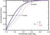 |
Fig. 12 Cumulative distribution of the combined mass of the two CO WDs merging within a Hubble time, for WD mergers having a combined mass higher than 1.4 M⊙, assuming different CE efficiencies. The lines have the same meaning as in Fig. 11. Vertical and horizontal lines indicate specific masses and cumulative fractions (Sect. 5.1.1). |
We investigate the influence of λce, which describes the mass distribution of the envelope, on the SN Ia rate. We also consider a specific extra energy source which is expressed by λion. In our standard model λce is a function of the type of star and its evolutionary state (Appendix A). As this prescription is not available in all BPS codes, λce is often taken to be 1 in other BPS studies.
Compared to the results of our standard model, the results of model B1 with λce = 1 show an increase in the integrated rate of only 3% and small changes in the different channels (Table 4). However, Table 5 shows that more SNe Ia occur at shorter delay times compared to the DTD from our standard model. If we assume λce equals 1 for all stars, the envelopes of HG and helium stars are less strongly bound than in our standard model, while those of stars on the GB and AGB are more strongly bound. This assumption leaves the systems interacting during the GB or AGB in a shorter orbit after the CE phase compared to our standard model. In double WD systems formed through the dominant evolutionary channel corresponding to region B, the secondary generally fills its Roche lobe for the first time during the GB or beyond. Consequently, the double WD systems formed through this evolutionary channel merge at relatively shorter delay times compared to our standard model.
During the CE phase, extra energy sources may facilitate the loss of the envelope. One example is the ionization energy which is modelled with λion. In model B2 we assume that 50% of the ionization energy is used to eject the envelope during the CE phase. This has the largest effect on the most massive progenitor systems and the systems that interact during the AGB. In general, the rate of the progenitor channels in which one star interacts during the AGB increases because AGB stars lose their envelope more easily during the CE phase. Consequently, SNe Ia formed through these progenitor channels originate from systems with shorter separations than in our standard model (e.g. region F of the DD channel and regions CH and CHe of both SD channels; see Table 4). Even though a variation of λion has a large effect on individual systems, the SN Ia rate increases by only 5% compared to our standard model.
5.2. Stability criterion of Roche-lobe overflowing stars
5.2.1. Helium stars
The evolution of helium stars is ill-constrained and therefore uncertainties remain in this evolutionary phase. We updated the stability criterion of Roche-lobe overflowing helium stars in the HG. In our standard model the stability criterion of He-HG stars is the same as the criterion of hydrogen-rich stars in the HG, which is expected as both types of stars have a similar envelope structure and therefore react similarly to mass loss. In older results published with our code the stability criterion of He-HG stars is equal to the criterion of He-GB stars (model C, Table 2). With this assumption stable RLOF from helium stars in the HG is less likely. As many results have been published with this assumption, we compare the effect of a variation of the stability criterion of Roche-lobe overflowing helium stars.
One might expect that a different prescription for Roche-lobe overflowing helium stars
mainly affects the SDHe channel, more specifically the progenitors with He-HG
donors, i.e. region BHe. Table 4 shows
that in model C region BHe is altered and the integrated rate of the
SDHe channel
decreases from  in our standard model to
  in model C. In our standard model only a small number of WD and helium star systems with
a mass ratio smaller than 0.87 form a SN Ia through the He-HG + WD channel because of
the high mass transfer rates involved, which explains the small difference in the rate
of the SDHe
channel (Fig. 5).
in model C. In our standard model only a small number of WD and helium star systems with
a mass ratio smaller than 0.87 form a SN Ia through the He-HG + WD channel because of
the high mass transfer rates involved, which explains the small difference in the rate
of the SDHe
channel (Fig. 5).
The helium star stability criterion mainly affects the DD channel, more specifically
region B2 (the
formation reversal channel, Table 4). This is
related to the crucial role of the stability criterion of helium stars in the formation
reversal channel because these systems go through a phase where both stars are helium
stars simultaneously. In this evolutionary channel, the difference between the stability
criteria determines whether a double WD system is formed in a short orbit or the binary
system merges during a CE phase. No SNe Ia are formed through the formation reversal
channel in model C and the integrated rate of region B decreases to
 ,
compared to
,
compared to  with our standard model.
Another difference between the results of our standard model and model C is the DTD (Figs. 7 and 13 and Table 5). The DTD of systems at short delay times changes substantially. The average rate at delay times between 100 Myr and 300 Myr is 0.052 SNuM with our standard model, while it is 0.31 SNuM with model C (Table 5). Our results suggest a t-1.3 relationship from about 400 Myr with the former model, and a t-1.1 relationship from about 115 Myr with model C. These differences originate from double WD systems that are formed after an evolved helium star has interacted with the first formed WD. In our standard model, when the helium star fills its Roche lobe mass transfer is stable. In model C, RLOF is unstable for some of these systems. In both cases a double WD system forms, but systems that result from a CE phase are in a shorter orbit afterwards than those that result from a phase of stable RLOF and therefore merge within a shorter time.
In conclusion, a different stability criterion of Roche-lobe overflowing helium stars affects 1) the DTD, more specifically the shorter delay times; and 2) the integrated rate by a factor of two. Model C has an integrated SN Ia rate of 2.3 × 10⁻⁴ M⊙-1 (Table 5), which is a factor of ten lower than the observed Maoz et al. (2011) rate.
5.2.2. Stars in the Hertzsprung gap
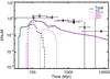 |
Fig. 13 Delay-time distribution of the different channels with model C which assumes Qcrit,He−HG = Qcrit,He−GB. Line styles and data points have the same meaning as in Fig. 7. |
A non-degenerate accreting star can undergo thermal expansion when it is brought out of thermal equilibrium. The binary can then evolve into a contact system, which possibly leads to a CE and/or merger. This process is more likely to occur in unequal mass binary systems (de Mink et al. 2007). However, the details of this process depend on the accretion efficiency and how energy is transported in the accreting star, both of which are uncertain. Because in our model the formulae used to determine the evolution of a star are based on stars in thermal equilibrium, we do not take thermal expansion into account. It is expected that the effect is equivalent to increasing the critical mass ratio Qcrit for donor stars in the HG (Table 2).
To estimate the effect of this uncertainty on the rate and the DTD, we consider model D with a different stability criterion of donor stars in the HG and He-HG with a non-degenerate accretor, Qcrit,HG = 0.5, compared to our standard model (Qcrit,HG = 0.25). This implies that stable RLOF of HG donors is less likely to occur, and therefore influences regions A, B, AH, BH, AHe, and BHe (Table 4). Because the systems that start RLOF during the HG have short initial separations and more binary systems evolve into a CE in model D compared to our standard model, fewer systems survive the first RLOF phase and form a SN Ia. In model D the integrated rate decreases by 23% compared to our standard model (Table 5).
5.3. Accretion efficiency
Apart from the stability criterion for RLOF, one of the main uncertainties in binary evolution is the RLOF accretion efficiency β. The RLOF accretion efficiency depends on the reaction of the accretor to mass accretion and on the angular momentum of the accreted material, which determines how fast the accretor spins up in reaction to accretion. It is uncertain how efficiently the star can lose the gained angular momentum. In our standard model the accretion efficiency is a function of the thermal timescale of the accretor (Eq. (14)) in which the uncertainty is expressed by a parameter σ which equals 10 in our standard model.
In models E1 and E2 we assume σ is 1 and 1000, respectively. A variation of the accretion efficiency of non-degenerate accretors has an impact on regions A to B of the DD channel and AH, BH, AHe, and BHe of the SD channels. In our standard model, mass transfer during RLOF is approximately conservative for high mass ratios because there is only a small difference between the thermal timescales of the two stars. In model E2 RLOF is approximately conservative for all mass ratios, while in model E1 RLOF is non-conservative over the entire mass ratio range. Consequently, a variation of σ mainly affects binary systems with unequal masses. A higher accretion efficiency increases the mass of the initially lowest mass companions after RLOF, which results in a higher SN Ia rate, and vice-versa. However, region A of the DD channel disappears in model E2 because the two WDs are in too long an orbit after conservative mass transfer to merge within a Hubble time. Compared to our standard model, the total integrated rate decreases by 12% assuming that the accretor can only accept accreted material with mass transfer rates lower than its thermal timescale (model E1, Table 4) and it increases by 14% assuming RLOF is approximately conservative (model E2, Table 4).
5.3.1. Unlimited accretion onto WDs
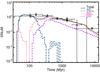 |
Fig. 14 Delay-time distribution of the SN Ia channels of model F1 with conservative mass transfer only to the WD. The line styles and data points have the same meaning as in Fig. 7. |
The models that are used to determine the WD retention efficiency assume a WD that has cooled for 108 yrs (Appendix B and Nomoto 1982). These models do not consider WDs with different temperatures, because of previous nova outbursts, for example, which can alter the accretion efficiency. For this and other reasons, the retention efficiency of WDs is uncertain and several models exist which describe this efficiency (Bours et al. 2013, and reference therein). Rather than investigating the effect of different retention efficiencies, as was done by Bours et al. (2013), we consider an extreme possibility where all mass transferred to the WD by RLOF remains on the WD and is burnt into carbon and oxygen (model F1). We do not consider this unlimited accretion onto a WD as a realistic model, but it represents an upper limit to the SD channel. In this model the critical mass ratio Qcrit for stable RLOF onto WDs is the same as onto non-degenerate stars (Table 2). During CE evolution we assume no mass is accreted. During phases of wind accretion, the amount accreted is calculated according to the Bondi-Hoyle prescription (Eq. (6)) for both degenerate and non-degenerate stars.
DD channel.
Unlimited accretion onto a WD does not significantly affect the rate of this channel, which is not determined by the amount of material accreted, but by how close together two WDs are formed. However, conservative RLOF results in changes in the initial parameter space compared to our non-conservative model (Table 4). The systems that undergo two CE phases (region F) are unaffected. The systems forming regions C to E in our standard model – which have stable mass transfer when the secondary fills its Roche lobe – disappear in model F1. In model F1, after the primary fills its Roche lobe during the GB or E-AGB, either RLOF is unstable when the secondary fills its Roche lobe and the binary evolves into a CE and merges, or RLOF is stable and everything is accreted by the WD which explodes as a SN Ia through the SDH channel. The DTD of the DD channel does not alter significantly; however, the overall rate decreases compared to our standard model by about 10% (Table 4 and Figs. 7 and 14).
SD channel.
For both SD channels large changes are expected because of the prominent role of the accretion efficiency in these channels. Figures 3 and 5 change significantly, because lower masses can provide enough mass to the WD through conservative mass transfer. This is partly counteracted by the fact that stable RLOF is only possible for somewhat lower donor masses.
Assuming conservative mass transfer towards the WD decreases the lower limit of donor masses in the SDH channel to 0.45 M⊙ (Fig. 3) and the minimum mass of WDs at formation to 0.3 M⊙. Consequently, the rate increases significantly in both models with conservative mass transfer. The SDH channel is dominant for delay times longer than 200 Myr (Fig. 14 and Table 5). The integrated rate is about three times larger than the rate of the DD channel with our standard model (Table 4).
In the SDHe channel the minimum He-star donor mass decreases to 0.7 M⊙, significantly lower than without conservative mass transfer (Fig. 5). The SDHe channel starts contributing to the DTD from about 45 Myr and continues until about 300 Myr in model F1 (Fig. 14 and Table 5). It remains the dominant channel for short delay times and increases by a factor of 10 compared to our standard model (Table 4).
Overall SN Ia rate.
The DTD is completely dominated by the SD channel. Prompt SNe Ia are mainly produced through the SDHe channel, while delayed SNe Ia are mainly produced through the SDH channel. The delayed component approximately follows a t-1 relation from 300 Myr; however, the rate drops slightly from about 5 Gyr. In the models with unlimited accretion onto the WD the observed DTD is well reproduced. The theoretical DTD has an average rate between 0 Gyr and 13.7 Gyr of 0.14 SNuM in model F1 (Figs. 14). The resulting integrated rate is compatible with the Maoz et al. (2011) rate (Table 4).
5.4. Angular momentum loss
When material is lost from a binary system it also removes angular momentum. Several prescriptions for angular momentum loss exist and influence the evolution of a binary system in different ways, depending on whether mass is lost through a stellar wind or RLOF. Below we discuss the effect of the uncertainties in angular momentum loss on both types of mass loss from a binary system (models G, H1, and H2) in the following sections.
5.4.1. Stellar wind
When mass is lost in a stellar wind, it is often assumed that this material does not interact with the binary system and that it is lost in a spherically symmetric way. However, this assumption only holds when winds are very fast compared to the orbital velocity of the system. Asymptotic giant branch stars have slow winds (speed ≈10−15 km s-1, see e.g. Vassiliadis & Wood 1993) and when they are in relatively close orbits the wind can interact with the orbit and remove specific orbital angular momentum from the binary system (Jahanara et al. 2005; Izzard et al. 2010).
In model G we assume that the material lost through a stellar wind carries twice the specific orbital angular momentum of the binary system. Some systems that do not interact in our standard model do interact in model G, which increases the rate of regions F, CH, and CHe (Table 4). Additionally, even though the DD channel remains dominant, the SDH channel, more specifically the WD+RG path, is more important at longer delay times (Table 5). Because angular momentum loss through a stellar wind does not affect the most common regions, the integrated rate of the two models differs by only 15%.
5.4.2. Roche-lobe overflow
Variation of the prescription of the amount of angular momentum lost when material is removed during a phase of stable RLOF affects those channels that have stable, non-conservative RLOF. Our model of accreting WDs that drive an optically thick wind requires that the material lost removes the specific orbital angular momentum of the accreting star (Sect. 2.2.5) and therefore we only vary the prescription of angular momentum loss during RLOF for other types of accretors.
A different assumption for angular momentum loss during RLOF affects regions A and B of the DD channel and AH, BH, AHe, and BHe of the SD channels. In general, when more angular momentum is lost compared to our standard model, initially wider systems become a SN Ia after a phase of stable RLOF, and vice versa. In model H1 mass loss takes the specific orbital angular momentum of the donor star, while in model H2 it is twice the specific orbital angular momentum of the binary. Although angular momentum loss during RLOF influences the most common evolutionary channels, it does not alter the rate drastically (Table 4).
5.5. Wind prescription
In our standard model, wind mass loss from stars up to the E-AGB is described by Reimers (1975, Eq. (1η = 0.5 and by Vassiliadis & Wood (1993) for the TP-AGB. Mass loss from helium stars is described by Reimers (1975) or Hamann & Koesterke (1998) depending on which of the two is stronger (Eq. (5)). Although the general trend of the evolution of the wind is known, the rate is not well constrained (Wachter et al. 2002). We discuss the effect of this uncertainty on the SN Ia rate below.
5.5.1. Stars on the E-AGB and helium stars
In model I the strength of the wind of stars up to the E-AGB and helium stars is greater (η = 5, Eq. (1)) than in our standard model (η = 0.5). This affects all the evolutionary channels, even those which show interaction on the TP-AGB because the prior evolution is altered. The DD channel is mainly affected in regions D to F because these binary systems have the strongest winds. Region F increases significantly, because more systems survive two CE phases as more material is lost before RLOF sets in. The SDH channel is mainly affected in region CH and the SDHe channel in regions BHe and CHe. The rate of both channels decreases because less material is accreted than through stable RLOF. In conclusion, the rate of the SD channel decreases in model I compared to our standard model. The opposite is true for the DD channel. The integrated SN Ia rate changes by only 6%.
5.5.2. TP-AGB
Several alternative prescriptions for wind mass loss during the TP-AGB phase are used to describe this evolution phase. Changing the wind prescription of stars on the TP-AGB only affects regions E and F of the DD channel and regions CH and CHe of the SD channels (Table 5, models J1 to J4). The high mass loss rate of Bloecker (1995, model J3 results in the shortest TP-AGB phase and forms the lowest mass WDs, which accordingly results in the lowest SN Ia rate of all the prescriptions for the TP-AGB under considerations. The prescription of Reimers (1975, with η = 1 during the TP-AGB, model J2 describes the longest wind phase, which results in the highest SN Ia rate. Because a change in the wind prescription of stars on the TP-AGB does not affect the most common evolution paths, a variation of it only changes the integrated rate up to 5%.
5.6. Combined effect of different binary parameters
In the above sections we tested separately the influence on the SN Ia rate of different binary evolution aspects. However, we do not necessarily expect that the effect of varying two parameters simultaneously is the same as the sum of the effects of varying each parameter separately. Therefore, we change some parameters under study at the same time and investigate their combined effect. We combine those parameters that have the largest influence on the SN Ia rate to determine the range of variation caused by uncertainties in binary evolution.
5.6.1. Common envelope efficiency and stability criterion of RLOF
Model P combines a low CE efficiency (αce = 0.2) and a different stability criterion of stars on the He-HG (Qcrit,He−HG = Qcrit,He−GB). Both assumptions separately decrease the rate (models A1 and C). When combined, the rate also decreases, but not by as much as the sum of the two effects separately. This occurs because model A1 and C both affect region B2 of the DD channel; moreover, in both models this region disappears. In model P, as in model A1, the SD channel dominates. The DTD is similar to that of model A1, except for an additional decrease in the DD channel because of the extra change of the stability criterion of Roche-lobe overflowing helium stars. The integrated rate decreases by about 65% compared to our standard model.
5.6.2. Accretion efficiency and angular momentum loss during wind mass transfer
Model Q combines a high Bondi-Hoyle accretion efficiency (αBH = 5, Eq. (6)) and a high angular momentum loss during wind mass loss (γwind = 2, Eq. (15)). It increases the SN Ia rate by 13%.
However, the rate of model Q is lower than that of model G. When more material is accreted during wind mass transfer and less material is lost, less angular momentum is lost from the system. Therefore, fewer double WD systems form in a short enough orbit to merge within a Hubble time in model Q compared to model G. The same holds for regions CH and CHe of both SD channels, where at WD formation the binary system is in a longer orbit in model Q than in model G. One might expect that the same reasoning holds for model L, in which less material is lost from the binary system compared to our standard model. However, in both model L and our standard model, when material is removed from the binary system the specific angular momentum of the donor star is lost, which is smaller for our progenitor systems than in models G and Q. Therefore, the rate of model L increases compared to our standard model because more material is accreted by the companion star.
6. Influence of initial binary distributions
The distribution functions of initial binary parameters are uncertain because of limitations in the different techniques used to determine them, such as difficulties in resolving binary companions or the incorrect determination of masses because of rotation (Scalo 1998; Kroupa 2001; Duchêne & Kraus 2013). In addition, it is not clear if the distribution functions are universal. Therefore we compare the theoretical SN Ia rates calculated assuming different initial binary distribution functions.
6.1. Initial mass ratio distribution
The initial mass ratio distribution of intermediate-mass stars is highly uncertain because of difficulties in the observations of the companion star (Duchêne & Kraus 2013). A flat distribution function of the initial mass ratio is widely used for BPS studies. However, some observations suggest a different distribution function for intermediate-mass stars, e.g. φ(q)∝q-0.4 (Kouwenhoven et al. 2007). In models N1 to N5 we investigate initial mass ratio distributions of this form with slopes between −1 and 1 (Table 1).
Figures 2, 4, and 6 show that most evolutionary channels require binary systems with a high initial mass ratio. Therefore the rate strongly depends on the distribution of the initial mass ratio and peaks when equal masses are favoured. Table 4 shows that the rate of every channel increases if the initial mass-ratio distribution is skewed towards equal masses, except in the most extreme case of model N5. In model N5 the rate corresponding to the regions that do not favour equal masses decreases compared to the rate of model N4, such as regions BH and BHe of the SD channels, although the overall rate of model N5 is higher compared to models N1 to N4. The integrated rate differs by a factor of 4.5 between the two extremes and is a factor of 4 to 17 times lower than the Maoz et al. (2011) rate. The most extreme model which strongly disfavours equal masses (model N1) is probably not realistic, as in this model about 50% of the systems with an initial primary mass between 2.5 M⊙ and 10 M⊙ have a secondary mass lower than 0.2 M⊙.
6.2. Initial mass function
The initial mass function (IMF) of Kroupa et al. (1993) is widely used, especially in SN Ia population synthesis studies. However, other prescriptions for the IMF exist. The IMF chosen defines the normalization of the population under study, therefore it is important to know which IMF is assumed when comparing results from different BPS codes and to realize how it affects the SN Ia rate (model O1 to O4). In general the IMF is described as a broken power-law function M−Γ, with Γ the slope of the power law. Kroupa et al. (1993) determine the IMF based on the low-mass stellar population in the Galactic disc. A break in the slope is observed around 0.5 M⊙, with Γ = 1.3 for systems with masses lower than 0.5 M⊙ and Γ = 2.2 for higher masses. An additional break arises around 1.0 M⊙, with a slope Γ = 2.7 above this mass.
Scalo (1998, model O1 defines an IMF mainly based on different galaxies and stellar associations, and his IMF is commonly used in older BPS studies. He finds that a stellar population contains a similar number of intermediate-mass stars with a mass between 1 M⊙ and 10 M⊙ compared to the IMF of Kroupa et al. (1993), but it contains fewer low-mass stars. As the number of intermediate-mass stars remains constant, while it decreases for the low-mass stars, the overall rate of model O1 increases compared to our standard model (Table 4).
Kroupa (2001, model O2 and Bell et al. (2003, model O4 find similar IMFs, based on the Galactic field and a large galaxy sample from the local universe, respectively. Both groups find a Salpeter-like IMF with Γ ≈ 2.35 for intermediate and massive stars, and a flatter slope below 0.5 M⊙ or 0.6 M⊙, respectively. A name commonly used for the IMF determined by Bell et al. (2003) is the diet Salpeter IMF and this is used for example by Maoz et al. (2012) and Graur & Maoz (2013) to extract the SN Ia rate. Models O2 and O4 show an increase in the SN Ia rate of approximately 40% compared to our standard model. Because the slope in the mass range between 2.5 M⊙ and 10 M⊙ is different from the slope in our standard model, the rate corresponding to the different evolution paths does not increase by the same amount, e.g. the rates from regions C and D of the DD channel change differently because the former favours less massive primaries than the latter.
Chabrier (2003, model O3 compares different present-day IMFs and shows that low-mass primaries (<1 M⊙) are distributed according to a log-normal function, while the best fit to the more massive stars is a power-law function in between the Salpeter function and the function determined by Scalo (1998) for the mass range between 1 M⊙ and 10 M⊙. This results in a stellar population that contains fewer low-mass primaries than our standard model. In model O3 our integrated rate increases by about 45% compared to our standard model and is about a factor of 3.5 lower than the Maoz et al. (2011) rate.
Although other prescriptions of the IMF result in an increase in the SN Ia rate with respect to our standard model, the rate of CC SNe increases as well. In models O1 to O4 the ratio of the SN Ia rate and the CC SN rate decreases compared to our standard model and is about a factor of three to seven lower than the observationally estimated ratio by Cappellaro et al. (1999, Table 3. The fraction η of intermediate-mass systems leading to a SN Ia varies between 2.3% and 2.5% between the different models (Table 3) and is about about a factor of six smaller than the observational estimate (Maoz 2008, Table 3), although this value is quite uncertain. Both comparisons in Table 3 indicate that although a variation of the IMF increases the integrated SN Ia rate, it does not reproduce other observational predictions regarding SN Ia.
Fraction η of the binary systems with a primary mass between 3 M⊙ and 8 M⊙ that result in a SN Ia and the expected SN Ia rate versus the CC SN rate of different models with varying IMFs compared with the observations.
6.3. Combining two distribution functions
In a population of stars, both the IMF and the initial mass ratio distribution can differ from our standard model. To test the most favourable situation we change both initial binary distribution functions simultaneously. We assume in model R an IMF according to Chabrier (2003) and an initial mass ratio distribution function with φ(q) ∝ q (see Tables 4 and 5).
The rate corresponding to all the regions increases in model R, similar to the amount expected from the combination of the two distributions separately. The overall rate is about a factor of three lower than the Maoz et al. (2011) rate and is compatible with the Maoz et al. (2012) rate (Fig. 15).
7. Discussion and conclusion
7.1. Progenitor evolution
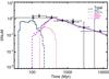 |
Fig. 15 Delay-time distribution of the SN Ia channels of model R, our most optimistic model, with an IMF according to Chabrier (2003) and initial mass ratio distribution φ(q) ∝ q. The line styles and data points have the same meaning as in Fig. 7. |
We find that the dominant progenitor evolutionary path for the DD channel is the Roche-lobe overflow path, in which the primary WD forms after a phase of stable RLOF and the secondary WD forms after a CE phase. In our standard model, this path accounts for 84% of the systems evolving though the DD channel, which is comparable to the fraction determined by Mennekens et al. (2010). In addition, 41% of the DD channel evolves through the formation reversal path, in which the initially less massive star forms the first WD (Toonen et al. 2012). This path is less common according to the results of Toonen et al. (2012), mainly because stable RLOF of helium stars in the HG is less likely to occur in the model of Toonen et al. (2012). The common envelope channel, which forms a double WD system after two CE phases, is uncommon and only accounts for about 2.4% of the DD channel in our standard model. This is lower than the fraction of about 17% found by Mennekens et al. (2010), which is partly explained by the fact that they only consider two formation scenarios for the DD channel. We also find another formation channel, in which the first WD forms after a CE phase and the secondary WD forms after a phase of stable RLOF, which accounts for about 13% of the DD systems in our standard model.
The dominant progenitor evolutionary path for the SD channel with hydrogen-rich donors (SDH) involves the formation of a WD after a CE phase and subsequent evolution through the WD+MS path. The least common path in our standard model is the WD+RG path, in contrast to the results of Ruiter et al. (2009) who find that this path is more common than the WD+MS path. A possible origin of the differences between these results is that in the models of Ruiter et al. (2009) stable RLOF of stars in the HG is less likely to occur, while stable RLOF of early GB stars is more likely to occur than in our model (Toonen et al. 2014). Mennekens et al. (2010) also find a DTD from the SDH channel dominated by the WD+MS path.
The dominant progenitor evolutionary path for the SD channel with helium-rich donors (SDHe) is through a phase of stable RLOF, which forms the WD, followed by a CE phase which forms the helium star donor. In our standard model and in most other models, the WD+He-MS path and WD+He-HG path contribute equally to the rate.
7.2. Theoretical SN Ia rate and comparison to other work
The DD channel contributes to the SN Ia rate from about 100 Myr up to a Hubble time. The different models agree that the respective DTD follows a t−x power law, with x = 1.3 in our standard model. The DD channel does not contribute at the shortest delay times. The DTD of SNe Ia at short delay times (≲100 Myr) is formed by the SDHe channel. Our models show that the SDH channel may contribute through the WD+MS path from about 70 Myr to 3500 Myr, depending on the mass range of the initially formed CO WDs, and until about 8000 Myr through the WD+RG path. The SD channel does not contribute to the longest delay times (≳8000 Myr). In our standard model, however, the SDH channel mainly contributes between 100 Myr and 500 Myr. Generally, the DD channel is the dominant formation channel, comprising 95% of the SN Ia rate in our standard model, but it cannot reproduce the prompt channel. Only the SDHe channel can account for SNe Ia at short delay times.
Additionally, our models show that the t-1 relation is not a standard characteristic of the DD channel. Because the DD channel is a combination of different progenitor channels, the DTD depends on the contribution of each of them (Sect. 5.1.1).
Although we produce SNe Ia both at short and long delay times, we do not reproduce the observed number of SNe Ia. We find an integrated rate which is a factor of 3 to 26 times lower than the Maoz et al. (2011) rate. However, the highest integrated rate we find, in model R, is compatible with the Maoz et al. (2012) rate.
The results of other groups are similar. Ruiter et al. (2009) find that the DD channel reproduces the observed t-1 relation, but is not able to reproduce the observed height of the DTD. Wang et al. (2009a) also discuss the SDHe channel and find that the SDHe channel is the progenitor channel responsible for the prompt SNe Ia. Greggio (2010) determines the DTD with an analytical approach. Her models which assume contributions of both the SD and the DD channel indicate that SNe Ia with delay times shorter than 0.1 Gyr originate from a combination of both channels, while at longer delay times the DD channel dominates. Greggio (2010) finds that the SD channel cannot reproduce the observed SN Ia rate at delay times longer than 10 Gyr.
Hachisu et al. (2008) describe the possibility of a radiation driven wind from the WD that strips extra material from the donor star and stabilizes RLOF more than the model adopted in this research. This results in more massive donor stars which can steadily transfer material to the WD. Mennekens et al. (2010) used this model to derive the DTD with a BPS code, but they could not reproduce the observed rate; their rate is at least a factor of three too low. In addition, the delayed component, produced by the SD WD+RG channel, drops at about 10 Gyr.
7.3. Uncertainties in binary evolution
The influence of uncertain aspects of single and binary star evolution on the SN Ia rate and DTD are studied in this paper. We find that most uncertainties only have a small effect on the SN Ia rate (<15%). This is because in our standard model the DD channel dominates, which is less sensitive to the masses of the WDs. However, the DD channel mainly depends on the spiral-in time after the formation of the two WDs and most uncertainties only marginally affect the spiral-in time. The uncertainties with the largest effect are the CE efficiency and helium star evolution, more specifically the stability of Roche-lobe-overflowing helium stars. Both result in a variation of at least a factor of two in the integrated rate (Table 5). Moreover, the ratio of the SD channel and the DD channel changes significantly when the CE efficiency is varied. The DD channel peaks when αce = 1 and the SD channel increases with decreasing CE efficiency. In the model with a low CE efficiency (αce = 0.2) the SD channel even dominates.
Other uncertainties are the initial binary distributions, where the two most extreme models give integrated rates that differ by a factor of five. The integrated rate of the model that combines the most optimistic distribution function of the initial primary mass and initial mass ratio is only a factor of three lower than the Maoz et al. (2011) rate. In addition, the number of SN Ia versus the number of CC SN remains at least a factor of 2.5 lower than estimated by Cappellaro et al. (1999).
We also consider the extreme situation of unlimited accretion onto a WD (model F1), which we do not believe to be realistic, but is adopted to determine an upper limit to the contribution of the SD channel. We find that rate corresponding to model F1 reproduces the Maoz et al. (2011) rate. More realistic assumptions yield a rate from the SD channel that is a factor of 10–100 lower. This does not indicate that the SD channel can be excluded, only that with normal assumptions it is hard to reproduce the observed rate with only the SD channel.
We mainly vary one parameter at a time to show its effect on the SN Ia progenitor evolution and the theoretical rate separately. We demonstrate that the result of changing two parameters at the same time is not always equal to the sum of the effects of each individual change (Sect. 5.6).
In addition, as mentioned in Sect. 4, the observed rate is also uncertain. Most recent observations show a rate that is about a factor of two and maybe a factor of four lower than the previously determined rate (Maoz et al. 2012; Graur & Maoz 2013; Perrett et al. 2012). Maoz et al. (2012) conclude that their rate at long delay times based on a sample dominated by field galaxies is more than 2σ lower than the rate at long delay times of Maoz et al. (2011) based on galaxies in cluster environments. In addition, the metallicities of clusters of galaxies (de Plaa et al. 2007) indicate a higher fraction of SNe Ia than in our own Galaxy. Maoz et al. (2012) suggest a possible enhancement of SNe Ia in cluster environments, while Sarazin (1986) suggests a difference in the IMF between the two types of environments. Even though it is not clear exactly where the differences come from, we point out that the theoretical rate found in our standard model is compatible with the lower limit of the observed rate.
7.4. Other uncertainties in the results
We show that variation of the binary physics assumptions has a great influence on the rate. However, our research does not give a complete overview of the uncertainties that dominate the SN Ia rate. Nelemans et al. (2013) show that different BPS codes show conflicting results, mainly for the SD channel. Recently four different BPS codes have been compared (Toonen et al. 2014), including ours. Toonen et al. (2014) show that the results found with the four codes are similar, when the same approximate assumptions are made. The differences that they find are caused by differences in the inherent assumptions in the codes, such as the initial-final mass relation, helium star evolution, the stability criterion of Roche-lobe overflowing stars and the mass transfer rate. In addition, Bours et al. (2013) show that the lack of understanding of the retention efficiency of WDs gives an integrated rate of the SD channel which varies between <10-7 and 1.5 × 10⁻⁴ M⊙-1.
Varying the binary fraction affects the rate as well. Our models assume a binary fraction of 100%, which is a reasonable assumptions for O and B stars (e.g. Kouwenhoven et al. 2007; Sana et al. 2012), but an overestimation for lower mass stars (e.g. Raghavan et al. 2010). As we do not expect that SNe Ia originate from single stars, the rate decreases when we adopt more realistic binary fractions. In addition, differences in the metallicity of the progenitor systems can alter the observed SN Ia rate. Toonen et al. (2012) discuss that a lower metallicity than solar does not affect the DTD from the DD channel; however, the integrated SN Ia rate increases with 30 to 60%. Meng et al. (2011) find that the DTD of the SDH channel is more delayed in models with lower metallicities than Solar.
There are also newly proposed channels possibly leading to SNe Ia which we did not consider for the work presented here, such as the core degenerate model (Kashi & Soker 2011; Ilkov & Soker 2012, 2013), in which a WD merges with the core of an AGB star during the CE phase; the double-detonation sub-Chandrasekhar explosion (Fink et al. 2010; Kromer et al. 2010), in which a WD explodes after the detonation of a thin helium layer accreted onto the WD with a low mass-transfer rate; the violent merger model (Pakmor et al. 2010, 2011), in which a massive enough WD explodes because of the accretion of material from another WD with an almost equal mass as the exploding WD; and the spin-up/spin-down model (Di Stefano et al. 2011; Hachisu et al. 2012), in which a WD gains angular momentum from the accreted material that spins up the WD, which can possible lead to super-Chandrasekhar WD and a delay between the explosion of the WD and the accretion of the material. Finally, we do not consider triple star evolution, which produces double WD mergers in eccentric orbits (Hamers et al. 2013) and, according to Rosswog et al. (2009), is an alternative scenario to produce SNe Ia. Even though we do not investigate the rate of these channels, it is expected that similar uncertainties to those discussed in this work influence the rate.
7.5. Outlook
Our models indicate that the progenitor evolution of SNe Ia does not consist of one evolutionary channel, but has many different branches with the relevance of each depending on different aspects of binary evolution. With upcoming supernova surveys we will get more detailed information on the differences between individual SNe Ia. Therefore, it is possible to gain insight in the sub-populations of SNe Ia. As a next step the characteristics of newly proposed progenitor channels should be investigated in more detail, including the properties of the merger products or the remaining companion stars. The outcome of such a study, combined with the results of this paper, can be linked with the different sub-populations of SNe Ia. However, when studying the rates of the other progenitor channels the uncertainties discussed in this work should always be kept in mind.
Online material
Appendix A: Mass distribution of the envelope
A method similar to that of Dewi & Tauris (2000) is used to calculate λce, by fitting it to detailed models from the STARS code (Eggleton 1971; Pols et al. 1995). The fitting formulae we use are also given and discussed in Izzard (2004).
For hydrogen-rich stars we distinguish between stars with radiative envelopes and stars
with deep convective envelopes. The expression for λce thus
depends on the mass of the convective envelope Menv expressed
in solar units, 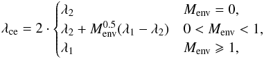 (A.1)where
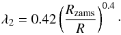 (A.2)The expression
for λ1 is more complicated and depends on
the type of star. For HG and GB stars we have
(A.2)The expression
for λ1 is more complicated and depends on
the type of star. For HG and GB stars we have
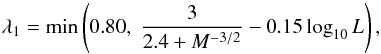 (A.3)where
M and
L are the
mass and luminosity of the star in solar units. For more evolved stars we define
(A.3)where
M and
L are the
mass and luminosity of the star in solar units. For more evolved stars we define
 (A.4)and
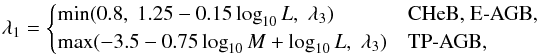 (A.5)with
the second expression for TP-AGB stars capped at a maximum λ1 of 1.0.
This results in typical values of λce ≈ 1.0−2.0 for stars on the GB or
AGB, and λce ≈ 0.25−0.75 for HG stars. For
helium stars no fit is available and we take λce = 0.5.
(A.5)with
the second expression for TP-AGB stars capped at a maximum λ1 of 1.0.
This results in typical values of λce ≈ 1.0−2.0 for stars on the GB or
AGB, and λce ≈ 0.25−0.75 for HG stars. For
helium stars no fit is available and we take λce = 0.5.
The loss of the envelope can be enhanced by using a fraction λion of the
ionization energy. In the code this is expressed by replacing λ1 in Eq.
(A.1) by
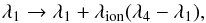 (A.6)where
0 ≤ λion ≤ 1 is a free parameter and
(A.6)where
0 ≤ λion ≤ 1 is a free parameter and
![Mathematical equation: \appendix \setcounter{section}{1} \begin{equation} \lambda_{4} = \max (\min[\lambda_{5}, \; 100], \; \lambda_{1}), \end{equation}](/articles/aa/full_html/2014/03/aa22714-13/aa22714-13-eq292.png) (A.7)where
λ5 is given by
(A.7)where
λ5 is given by
![Mathematical equation: \appendix \setcounter{section}{1} \begin{equation} \lambda_{5} = \frac{1}{a + \arctan(b[c - \log_{10} L]) + d(\log_{10} L - 2)}\cdot \end{equation}](/articles/aa/full_html/2014/03/aa22714-13/aa22714-13-eq294.png) (A.8)The coefficients
a –
d depend
on stellar type and mass as follows:
(A.8)The coefficients
a –
d depend
on stellar type and mass as follows:
![Mathematical equation: \appendix \setcounter{section}{1} \begin{equation} a = \begin{cases} \min(-0.5, \; 1.2\,[\log_{10} M - 0.25]^{2} - 0.7) & \text{HG, GB,} \\ \max(-0.5, \; -0.2 - \log_{10} M) & \text{CHeB, AGB,} \end{cases} \end{equation}](/articles/aa/full_html/2014/03/aa22714-13/aa22714-13-eq295.png) (A.9)
(A.9) (A.10)
 (A.11)and
![Mathematical equation: \appendix \setcounter{section}{1} \begin{equation} d = \begin{cases} \max(0, \; \min[0.15, \; 0.15 - 0.25\log_{10} M]) & \text{HG, GB,} \\ 0 & \text{CHeB, AGB.} \end{cases} \end{equation}](/articles/aa/full_html/2014/03/aa22714-13/aa22714-13-eq298.png) (A.12)
(A.12)
Appendix B: Accretion efficiency of WDs
Material that is transferred to a WD at a rate Ṁtr can only be burnt by the WD at a specific rate (Nomoto 1982). If the mass transfer rate is lower than this specific rate the material is added onto the surface and later on ejected in a nova explosion. When the material is transferred to the WD at a higher rate, we assume that the material that is not burnt is blown away through an optically thick wind from the accreting WD (Hachisu et al. 1996).
When He-rich material is accreted, it burns into carbon and oxygen. The net accretion
efficiency (ηHe) is written 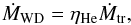 (B.1)where Ṁtr is the
mass transfer rate and ṀWD the net mass growth of the WD.
(B.1)where Ṁtr is the
mass transfer rate and ṀWD the net mass growth of the WD.
When hydrogen-rich material is transferred to the WD the net accretion efficiency
(ηHeηH) is
written 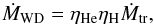 (B.2)because first
hydrogen is burnt into helium, and subsequently helium is burnt into carbon and oxygen.
(B.2)because first
hydrogen is burnt into helium, and subsequently helium is burnt into carbon and oxygen.
The accretion efficiencies for hydrogen and helium burning, ηH and
ηHe, are calculated following Hachisu et al. (1999)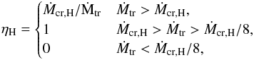 (B.3)where
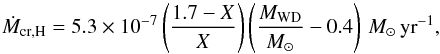 (B.4)and where
X is the
hydrogen abundance, and
(B.4)and where
X is the
hydrogen abundance, and 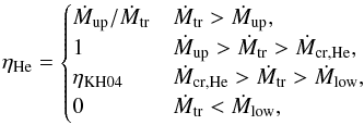 (B.5)where
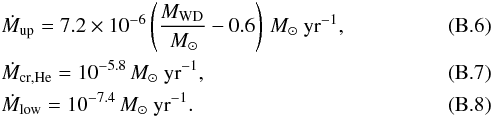 The
expression for Ṁup is based on Nomoto (1982) and Ṁcr,He and
Ṁlow are based on the models of Kato & Hachisu (2004); more specifically,
Ṁlow is the lower limit of the models
that have He-shell flashes. The accretion efficiency ηKH04 is based
on the models for He-shell flashes of Kato &
Hachisu (2004), implemented in a similar way as in Meng et al. (2009). This process is limited by the Eddington limit
for accretion.
The
expression for Ṁup is based on Nomoto (1982) and Ṁcr,He and
Ṁlow are based on the models of Kato & Hachisu (2004); more specifically,
Ṁlow is the lower limit of the models
that have He-shell flashes. The accretion efficiency ηKH04 is based
on the models for He-shell flashes of Kato &
Hachisu (2004), implemented in a similar way as in Meng et al. (2009). This process is limited by the Eddington limit
for accretion.
Acknowledgments
J.S.W.C. would like to thank Alex Chiotellis for the discussions about wind mass loss and for his help in determining the critical mass ratios of accreting WDs. We would also like to thank the referee, Zhanwen Han, for the useful feedback. The work of J.S.W.C. was supported by the Dutch Research School for Astronomy (NOVA). R.G.I. thanks the Alexander von Humboldt Foundation for funding his current position.
References
- Bell, E. F., McIntosh, D. H., Katz, N., & Weinberg, M. D. 2003, ApJS, 149, 289 [NASA ADS] [CrossRef] [Google Scholar]
- Bloecker, T. 1995, A&A, 297, 727 [Google Scholar]
- Bloom, J. S., Kasen, D., Shen, K. J., et al. 2012, ApJ, 744, L17 [NASA ADS] [CrossRef] [Google Scholar]
- Bondi, H., & Hoyle, F. 1944, MNRAS, 104, 273 [NASA ADS] [CrossRef] [Google Scholar]
- Bours, M. C. P., Toonen, S., & Nelemans, G. 2013, A&A, 552, A24 [NASA ADS] [CrossRef] [EDP Sciences] [Google Scholar]
- Cappellaro, E., Evans, R., & Turatto, M. 1999, A&A, 351, 459 [NASA ADS] [Google Scholar]
- Chabrier, G. 2003, PASP, 115, 763 [NASA ADS] [CrossRef] [Google Scholar]
- Chen, X., Jeffery, C. S., Zhang, X., & Han, Z. 2012, ApJ, 755, L9 [NASA ADS] [CrossRef] [Google Scholar]
- Chevalier, R. A. 2012, ApJ, 752, L2 [NASA ADS] [CrossRef] [Google Scholar]
- Chiotellis, A., Schure, K. M., & Vink, J. 2012, A&A, 537, A139 [NASA ADS] [CrossRef] [EDP Sciences] [Google Scholar]
- Chomiuk, L., Soderberg, A. M., Moe, M., et al. 2012, ApJ, 750, 164 [NASA ADS] [CrossRef] [Google Scholar]
- Dan, M., Rosswog, S., Brüggen, M., & Podsiadlowski, P. 2014, MNRAS, 438, 14 [NASA ADS] [CrossRef] [Google Scholar]
- Davis, P. J., Kolb, U., & Knigge, C. 2012, MNRAS, 419, 287 [NASA ADS] [CrossRef] [Google Scholar]
- De Marco, O., Passy, J.-C., Moe, M., et al. 2011, MNRAS, 411, 2277 [NASA ADS] [CrossRef] [Google Scholar]
- de Mink, S. E., Pols, O. R., & Hilditch, R. W. 2007, A&A, 467, 1181 [NASA ADS] [CrossRef] [EDP Sciences] [Google Scholar]
- de Plaa, J., Werner, N., Bleeker, J. A. M., et al. 2007, A&A, 465, 345 [NASA ADS] [CrossRef] [EDP Sciences] [Google Scholar]
- Dewi, J. D. M., & Tauris, T. M. 2000, A&A, 360, 1043 [NASA ADS] [Google Scholar]
- Di Stefano, R. 2010, ApJ, 712, 728 [NASA ADS] [CrossRef] [Google Scholar]
- Di Stefano, R., Voss, R., & Claeys, J. S. W. 2011, ApJ, 738, L1 [NASA ADS] [CrossRef] [Google Scholar]
- Dilday, B., Howell, D. A., Cenko, S. B., et al. 2012, Science, 337, 942 [NASA ADS] [CrossRef] [Google Scholar]
- Duchêne, G., & Kraus, A. 2013, ARA&A, 51, 269 [Google Scholar]
- Eggleton, P. P. 1971, MNRAS, 151, 351 [NASA ADS] [CrossRef] [Google Scholar]
- Eggleton, P. P. 1983, ApJ, 268, 368 [NASA ADS] [CrossRef] [Google Scholar]
- Eggleton, P. 2006, Evolutionary Processes in Binary and Multiple Stars (Cambridge: Cambridge Univ. Press) [Google Scholar]
- Fink, M., Röpke, F. K., Hillebrandt, W., et al. 2010, A&A, 514, A53 [NASA ADS] [CrossRef] [EDP Sciences] [Google Scholar]
- García-Senz, D., Badenes, C., & Serichol, N. 2012, ApJ, 745, 75 [NASA ADS] [CrossRef] [Google Scholar]
- Gilfanov, M., & Bogdán, Á. 2010, Nature, 463, 924 [NASA ADS] [CrossRef] [PubMed] [Google Scholar]
- Glebbeek, E., Pols, O. R., & Hurley, J. R. 2008, A&A, 488, 1007 [NASA ADS] [CrossRef] [EDP Sciences] [Google Scholar]
- Graur, O., & Maoz, D. 2013, MNRAS, 430, 1746 [NASA ADS] [CrossRef] [Google Scholar]
- Graur, O., Poznanski, D., Maoz, D., et al. 2011, MNRAS, 417, 916 [NASA ADS] [CrossRef] [Google Scholar]
- Greggio, L. 2010, MNRAS, 406, 22 [NASA ADS] [CrossRef] [Google Scholar]
- Hachisu, I., Kato, M., & Nomoto, K. 1996, ApJ, 470, L97 [NASA ADS] [CrossRef] [Google Scholar]
- Hachisu, I., Kato, M., & Nomoto, K. 1999, ApJ, 522, 487 [NASA ADS] [CrossRef] [Google Scholar]
- Hachisu, I., Kato, M., & Nomoto, K. 2008, ApJ, 683, L127 [NASA ADS] [CrossRef] [Google Scholar]
- Hachisu, I., Kato, M., Saio, H., & Nomoto, K. 2012, ApJ, 744, 69 [NASA ADS] [CrossRef] [Google Scholar]
- Hamann, W.-R., & Koesterke, L. 1998, A&A, 335, 1003 [NASA ADS] [Google Scholar]
- Hamann, W.-R., Koesterke, L., & Wessolowski, U. 1995, A&A, 299, 151 [NASA ADS] [Google Scholar]
- Hamers, A. S., Pols, O. R., Claeys, J. S. W., & Nelemans, G. 2013, MNRAS, 704 [Google Scholar]
- Hamuy, M., Phillips, M. M., Suntzeff, N. B., et al. 2003, Nature, 424, 651 [NASA ADS] [CrossRef] [Google Scholar]
- Han, Z., & Podsiadlowski, P. 2004, MNRAS, 350, 1301 [NASA ADS] [CrossRef] [Google Scholar]
- Howell, D. A. 2011, Nature Commun., 2, 350 [Google Scholar]
- Howell, D. A., Sullivan, M., Nugent, P. E., et al. 2006, Nature, 443, 308 [NASA ADS] [CrossRef] [PubMed] [Google Scholar]
- Hurley, J. R., Pols, O. R., & Tout, C. A. 2000, MNRAS, 315, 543 [NASA ADS] [CrossRef] [Google Scholar]
- Hurley, J. R., Tout, C. A., & Pols, O. R. 2002, MNRAS, 329, 897 [NASA ADS] [CrossRef] [Google Scholar]
- Iben, Jr., I., & Tutukov, A. V. 1984, ApJS, 54, 335 [NASA ADS] [CrossRef] [Google Scholar]
- Ilkov, M., & Soker, N. 2012, MNRAS, 419, 1695 [NASA ADS] [CrossRef] [Google Scholar]
- Ilkov, M., & Soker, N. 2013, MNRAS, 428, 579 [NASA ADS] [CrossRef] [Google Scholar]
- Ivanova, N. 2011, in Evolution of Compact Binaries, ed. L. Schmidtobreick, M. R. Schreiber, & C. Tappert, ASP Conf. Ser., 447, 91 [Google Scholar]
- Izzard, R. G. 2004, Ph.D. Thesis, Univ. of Cambridge [Google Scholar]
- Izzard, R. G., Tout, C. A., Karakas, A. I., & Pols, O. R. 2004, MNRAS, 350, 407 [NASA ADS] [CrossRef] [Google Scholar]
- Izzard, R. G., Dray, L. M., Karakas, A. I., Lugaro, M., & Tout, C. A. 2006, A&A, 460, 565 [NASA ADS] [CrossRef] [EDP Sciences] [Google Scholar]
- Izzard, R. G., Glebbeek, E., Stancliffe, R. J., & Pols, O. R. 2009, A&A, 508, 1359 [NASA ADS] [CrossRef] [EDP Sciences] [Google Scholar]
- Izzard, R. G., Dermine, T., & Church, R. P. 2010, A&A, 523, A10 [NASA ADS] [CrossRef] [EDP Sciences] [Google Scholar]
- Jahanara, B., Mitsumoto, M., Oka, K., et al. 2005, A&A, 441, 589 [NASA ADS] [CrossRef] [EDP Sciences] [Google Scholar]
- Karakas, A. I., Lattanzio, J. C., & Pols, O. R. 2002, PASA, 19, 515 [NASA ADS] [CrossRef] [Google Scholar]
- Kashi, A., & Soker, N. 2011, MNRAS, 417, 1466 [NASA ADS] [CrossRef] [Google Scholar]
- Kato, M., & Hachisu, I. 2004, ApJ, 613, L129 [NASA ADS] [CrossRef] [Google Scholar]
- Kerzendorf, W. E., Schmidt, B. P., Asplund, M., et al. 2009, ApJ, 701, 1665 [NASA ADS] [CrossRef] [Google Scholar]
- Kobulnicky, H. A., & Fryer, C. L. 2007, ApJ, 670, 747 [NASA ADS] [CrossRef] [Google Scholar]
- Kouwenhoven, M. B. N., Brown, A. G. A., Portegies Zwart, S. F., & Kaper, L. 2007, A&A, 474, 77 [NASA ADS] [CrossRef] [EDP Sciences] [Google Scholar]
- Kromer, M., Sim, S. A., Fink, M., et al. 2010, ApJ, 719, 1067 [NASA ADS] [CrossRef] [Google Scholar]
- Kroupa, P. 2001, MNRAS, 322, 231 [NASA ADS] [CrossRef] [Google Scholar]
- Kroupa, P., Tout, C. A., & Gilmore, G. 1993, MNRAS, 262, 545 [NASA ADS] [CrossRef] [Google Scholar]
- Lada, C. J. 2006, ApJ, 640, L63 [NASA ADS] [CrossRef] [Google Scholar]
- Leonard, D. C. 2007, ApJ, 670, 1275 [NASA ADS] [CrossRef] [Google Scholar]
- Li, W., Bloom, J. S., Podsiadlowski, P., et al. 2011a, Nature, 480, 348 [NASA ADS] [CrossRef] [Google Scholar]
- Li, W., Chornock, R., Leaman, J., et al. 2011b, MNRAS, 412, 1473 [NASA ADS] [CrossRef] [Google Scholar]
- Mannucci, F., Della Valle, M., Panagia, N., et al. 2005, A&A, 433, 807 [NASA ADS] [CrossRef] [EDP Sciences] [Google Scholar]
- Mannucci, F., Della Valle, M., & Panagia, N. 2006, MNRAS, 370, 773 [NASA ADS] [CrossRef] [Google Scholar]
- Maoz, D. 2008, MNRAS, 384, 267 [NASA ADS] [CrossRef] [Google Scholar]
- Maoz, D., & Mannucci, F. 2012, PASA, 29, 447 [NASA ADS] [CrossRef] [Google Scholar]
- Maoz, D., Sharon, K., & Gal-Yam, A. 2010, ApJ, 722, 1879 [Google Scholar]
- Maoz, D., Mannucci, F., Li, W., et al. 2011, MNRAS, 412, 1508 [NASA ADS] [CrossRef] [Google Scholar]
- Maoz, D., Mannucci, F., & Brandt, T. D. 2012, MNRAS, 426, 3282 [NASA ADS] [CrossRef] [Google Scholar]
- Margutti, R., Soderberg, A. M., Chomiuk, L., et al. 2012, ApJ, 751, 134 [NASA ADS] [CrossRef] [Google Scholar]
- Meng, X., Chen, X., & Han, Z. 2009, MNRAS, 395, 2103 [NASA ADS] [CrossRef] [Google Scholar]
- Meng, X. C., Li, Z. M., & Yang, W. M. 2011, PASJ, 63, L31 [NASA ADS] [CrossRef] [Google Scholar]
- Mennekens, N., Vanbeveren, D., De Greve, J. P., & De Donder, E. 2010, A&A, 515, A89 [NASA ADS] [CrossRef] [EDP Sciences] [Google Scholar]
- Nelemans, G., Toonen, S., & Bours, M. 2013, in Binary Paths to Type Ia Supernovae Explosions, IAU Symp., 281, 225 [Google Scholar]
- Nielsen, M. T. B., Dominik, C., Nelemans, G., & Voss, R. 2013, A&A, 549, A32 [NASA ADS] [CrossRef] [EDP Sciences] [Google Scholar]
- Nomoto, K. 1982, ApJ, 253, 798 [NASA ADS] [CrossRef] [Google Scholar]
- Nomoto, K., & Kondo, Y. 1991, ApJ, 367, L19 [NASA ADS] [CrossRef] [Google Scholar]
- Öpik, E. 1924, Publ. of the Tartu Astrofizica Obs., 25, 1 [Google Scholar]
- Pakmor, R., Hachinger, S., Röpke, F. K., & Hillebrandt, W. 2011, A&A, 528, A117 [NASA ADS] [CrossRef] [EDP Sciences] [Google Scholar]
- Pakmor, R., Kromer, M., Röpke, F. K., et al. 2010, Nature, 463, 61 [NASA ADS] [CrossRef] [PubMed] [Google Scholar]
- Pakmor, R., Kromer, M., Taubenberger, S., & Springel, V. 2013, ApJ, 770, L8 [NASA ADS] [CrossRef] [Google Scholar]
- Passy, J.-C., De Marco, O., Fryer, C. L., et al. 2012, ApJ, 744, 52 [NASA ADS] [CrossRef] [Google Scholar]
- Patat, F., Benetti, S., Justham, S., et al. 2007, A&A, 474, 931 [NASA ADS] [CrossRef] [EDP Sciences] [Google Scholar]
- Patat, F., Cordiner, M. A., Cox, N. L. J., et al. 2013, A&A, 549, A62 [NASA ADS] [CrossRef] [EDP Sciences] [Google Scholar]
- Perlmutter, S., Aldering, G., Goldhaber, G., et al. 1999, ApJ, 517, 565 [NASA ADS] [CrossRef] [Google Scholar]
- Perrett, K., Sullivan, M., Conley, A., et al. 2012, AJ, 144, 59 [NASA ADS] [CrossRef] [Google Scholar]
- Phillips, M. M. 1993, ApJ, 413, L105 [NASA ADS] [CrossRef] [Google Scholar]
- Pols, O. R., Tout, C. A., Eggleton, P. P., & Han, Z. 1995, MNRAS, 274, 964 [NASA ADS] [CrossRef] [Google Scholar]
- Pols, O. R., Schroder, K.-P., Hurley, J. R., Tout, C. A., & Eggleton, P. P. 1998, MNRAS, 298, 525 [NASA ADS] [CrossRef] [Google Scholar]
- Pritchet, C. J., Howell, D. A., & Sullivan, M. 2008, ApJ, 683, L25 [NASA ADS] [CrossRef] [Google Scholar]
- Raghavan, D., McAlister, H. A., Henry, T. J., et al. 2010, ApJS, 190, 1 [NASA ADS] [CrossRef] [EDP Sciences] [Google Scholar]
- Reimers, D. 1975, Mem. Soc. Roy. Sci. Liège, 8, 369 [Google Scholar]
- Riess, A. G., Press, W. H., & Kirshner, R. P. 1996, ApJ, 473, 88 [NASA ADS] [CrossRef] [Google Scholar]
- Riess, A. G., Filippenko, A. V., Challis, P., et al. 1998, AJ, 116, 1009 [NASA ADS] [CrossRef] [Google Scholar]
- Rosswog, S., Kasen, D., Guillochon, J., & Ramirez-Ruiz, E. 2009, ApJ, 705, L128 [NASA ADS] [CrossRef] [Google Scholar]
- Ruiter, A. J., Belczynski, K., & Fryer, C. 2009, ApJ, 699, 2026 [NASA ADS] [CrossRef] [Google Scholar]
- Ruiz-Lapuente, P., Comeron, F., Méndez, J., et al. 2004, Nature, 431, 1069 [NASA ADS] [CrossRef] [PubMed] [Google Scholar]
- Sana, H., de Mink, S. E., de Koter, A., et al. 2012, Science, 337, 444 [Google Scholar]
- Sarazin, C. L. 1986, Rev. Mod. Phys., 58, 1 [NASA ADS] [CrossRef] [Google Scholar]
- Scalo, J. 1998, in The Stellar Initial Mass Function, eds. G. Gilmore, & D. Howell, ASP Conf. Ser., 142, 201 [Google Scholar]
- Scannapieco, E., & Bildsten, L. 2005, ApJ, 629, L85 [NASA ADS] [CrossRef] [Google Scholar]
- Schaefer, B. E., & Pagnotta, A. 2012, Nature, 481, 164 [NASA ADS] [CrossRef] [Google Scholar]
- Shen, K. J., Guillochon, J., & Foley, R. J. 2013, ApJ, 770, L35 [NASA ADS] [CrossRef] [Google Scholar]
- Soberman, G. E., Phinney, E. S., & van den Heuvel, E. P. J. 1997, A&A, 327, 620 [NASA ADS] [Google Scholar]
- Soker, N., Kashi, A., García-Berro, E., Torres, S., & Camacho, J. 2013, MNRAS, 431, 1541 [NASA ADS] [CrossRef] [Google Scholar]
- Sternberg, A., Gal-Yam, A., Simon, J. D., et al. 2011, Science, 333, 856 [NASA ADS] [CrossRef] [Google Scholar]
- Toonen, S., Nelemans, G., & Portegies Zwart, S. 2012, A&A, 546, A70 [NASA ADS] [CrossRef] [EDP Sciences] [Google Scholar]
- Toonen, S., Claeys, J. S. W., Mennekens, N., & Ruiter, A. J. 2014, A&A, 562, A14 [NASA ADS] [CrossRef] [EDP Sciences] [Google Scholar]
- Totani, T., Morokuma, T., Oda, T., Doi, M., & Yasuda, N. 2008, PASJ, 60, 1327 [NASA ADS] [CrossRef] [Google Scholar]
- Tout, C. A., & Eggleton, P. P. 1988, MNRAS, 231, 823 [NASA ADS] [CrossRef] [Google Scholar]
- van den Heuvel, E. P. J., Bhattacharya, D., Nomoto, K., & Rappaport, S. A. 1992, A&A, 262, 97 [NASA ADS] [Google Scholar]
- van Loon, J. T., Cioni, M.-R. L., Zijlstra, A. A., & Loup, C. 2005, A&A, 438, 273 [NASA ADS] [CrossRef] [EDP Sciences] [Google Scholar]
- Vassiliadis, E., & Wood, P. R. 1993, ApJ, 413, 641 [NASA ADS] [CrossRef] [Google Scholar]
- Wachter, A., Schröder, K.-P., Winters, J. M., Arndt, T. U., & Sedlmayr, E. 2002, A&A, 384, 452 [NASA ADS] [CrossRef] [EDP Sciences] [Google Scholar]
- Wang, B., & Han, Z.-W. 2010, Res. Astron. Astrophys.., 10, 235 [NASA ADS] [CrossRef] [Google Scholar]
- Wang, B., Chen, X., Meng, X., & Han, Z. 2009a, ApJ, 701, 1540 [NASA ADS] [CrossRef] [Google Scholar]
- Wang, B., Meng, X., Chen, X., & Han, Z. 2009b, MNRAS, 395, 847 [NASA ADS] [CrossRef] [Google Scholar]
- Wang, B., Li, X.-D., & Han, Z.-W. 2010, MNRAS, 401, 2729 [NASA ADS] [CrossRef] [Google Scholar]
- Webbink, R. F. 1984, ApJ, 277, 355 [NASA ADS] [CrossRef] [Google Scholar]
- Weidemann, V. 2000, A&A, 363, 647 [NASA ADS] [Google Scholar]
- Whelan, J., & Iben, Jr., I. 1973, ApJ, 186, 1007 [NASA ADS] [CrossRef] [Google Scholar]
- Whyte, C. A., & Eggleton, P. P. 1980, MNRAS, 190, 801 [NASA ADS] [Google Scholar]
- Yoon, S.-C., & Langer, N. 2005, A&A, 435, 967 [NASA ADS] [CrossRef] [EDP Sciences] [Google Scholar]
- Yungelson, L. R., & Livio, M. 2000, ApJ, 528, 108 [CrossRef] [Google Scholar]
- Zorotovic, M., Schreiber, M. R., Gänsicke, B. T., & Nebot Gómez-Morán, A. 2010, A&A, 520, A86 [NASA ADS] [CrossRef] [EDP Sciences] [Google Scholar]
All Tables
Critical mass ratio Qcrit for stable RLOF for different types of donor stars, in the case of a non-degenerate and a degenerate accretor.
Fraction η of the binary systems with a primary mass between 3 M⊙ and 8 M⊙ that result in a SN Ia and the expected SN Ia rate versus the CC SN rate of different models with varying IMFs compared with the observations.
All Figures
|
Fig. 1 Initial (Mi) versus final (Mf) mass of single stars that become CO WDs for different TP-AGB models (Sect. 2.1.1). The dotted line shows the results of the Hurley et al. (2000) models, the full line shows the results for the fits to the Karakas et al. (2002) models, and the dashed line shows our model. |
| In the text | |
|
Fig. 2 Initial separation (ai) versus initial mass of the primary star (Mi, left) and versus initial mass ratio (M2,i/M1,i, right) of systems that form SNe Ia through the DD channel in our standard model (Sect. 2). Number density (greyscale) represents the number of systems normalized to the total number of systems forming a SN Ia through the DD channel. Lines show the minimum separation (assuming q = 1) for which the primary fills its Roche lobe at a certain stage of evolution, as indicated. Symbols A–F indicate differences in the evolutionary stage when the primary fills its Roche lobe and in the number of CE phases necessary to evolve to a SN Ia: A = HG, no CE; B = HG, 1 CE (the difference between B1 and B2 is based on which of the two stars first forms a WD); C = GB, 1 CE; D = E-AGB, 1 CE; E = TP-AGB, 1 CE; F = TP-AGB, 2 CEs. |
| In the text | |
|
Fig. 3 Donor mass (Md) versus separation (a) at the moment of formation of the CO WD of the systems producing SNe Ia through the SDH channel, for different CO WD masses: 1.15 M⊙ (solid line), 1.0 M⊙ (dash-dotted line), and 0.8 M⊙ (dotted line). The greyscale shows how these regions are populated in our standard model. Labels indicate the different stellar types of donors stars. |
| In the text | |
|
Fig. 4 As Fig. 2 for systems that form SNe Ia through the SDH channel. Symbols AH, BH, and CH indicate groups which are distinguished based on the evolutionary stage when the primary fills its Roche lobe and the number of CE phases necessary to evolve to a SN Ia: AH = HG, no CE; BH = end of HG/GB, 1 CE; CH = TP-AGB, 1 CE. |
| In the text | |
|
Fig. 5 As Fig. 3 for systems at the formation of the WD and He-MS binary that produce SNe Ia through the SDHe channel. |
| In the text | |
|
Fig. 6 As Fig. 2 for systems that form SNe Ia through the SDHe channel. Symbols AHe, BHe, and CHe indicate groups that are distinguished based on the evolutionary stage when the primary fills its Roche lobe, the number of CE phases necessary to evolve to a SN Ia, and the type of donor star transferring mass to the CO WD: AHe = HG, no CE, with He-MS donors; BHe = HG, 1 CE, with He-HG donors; CHe = TP-AGB, 1 CE. |
| In the text | |
|
Fig. 7 Delay-time distribution of the different channels with our standard model (Sect. 2): the SDHe channel (blue dash-dotted line), the SDH channel (red dotted line), the DD channel (purple dashed line), and the overall SN Ia rate (black thin full line), which is the sum of the three channels. The rate is presented in units of SNuM which is the SN Ia rate per 100 yr per 1010 M⊙ in stars. Data points represent the observed DTD from Totani et al. (2008, triangles) and Maoz et al. (2011, squares). |
| In the text | |
|
Fig. 8 Number of SNe Ia (NSN) per unit mass versus time, with our standard model (Sect. 2). Line styles have the same meaning as in Fig. 7. Data points show the integrated rate (over a Hubble time) determined by Maoz et al. (2011, diamond), Maoz et al. (2012, square), and Graur & Maoz (2013, triangle). |
| In the text | |
|
Fig. 9 Cumulative distribution of the combined mass of the two CO WDs merging within a Hubble time for WD mergers having a combined mass greater than 1.4 M⊙ in our standard model. The lines indicate specific masses and cumulative fractions (Sect. 4.1). |
| In the text | |
|
Fig. 10 DTD of the SD channel for the assumptions discussed in Sect. 2 and with variable CE efficiency αce: 1 (black full line), 0.5 (blue dashed line), and 0.2 (red dotted line). The thick lines show the SDHe channel, while the thin lines show SDH channel. Data points have the same meaning as in Fig. 7. |
| In the text | |
|
Fig. 11 DTD of the DD channel for our standard model (Sect. 2) and with variable CE efficiency αce: 3 (black full line), 1 (blue dashed line), and 0.5 (red dotted line). Data points have the same meaning as in Fig. 7. |
| In the text | |
|
Fig. 12 Cumulative distribution of the combined mass of the two CO WDs merging within a Hubble time, for WD mergers having a combined mass higher than 1.4 M⊙, assuming different CE efficiencies. The lines have the same meaning as in Fig. 11. Vertical and horizontal lines indicate specific masses and cumulative fractions (Sect. 5.1.1). |
| In the text | |
|
Fig. 13 Delay-time distribution of the different channels with model C which assumes Qcrit,He−HG = Qcrit,He−GB. Line styles and data points have the same meaning as in Fig. 7. |
| In the text | |
|
Fig. 14 Delay-time distribution of the SN Ia channels of model F1 with conservative mass transfer only to the WD. The line styles and data points have the same meaning as in Fig. 7. |
| In the text | |
|
Fig. 15 Delay-time distribution of the SN Ia channels of model R, our most optimistic model, with an IMF according to Chabrier (2003) and initial mass ratio distribution φ(q) ∝ q. The line styles and data points have the same meaning as in Fig. 7. |
| In the text | |
Current usage metrics show cumulative count of Article Views (full-text article views including HTML views, PDF and ePub downloads, according to the available data) and Abstracts Views on Vision4Press platform.
Data correspond to usage on the plateform after 2015. The current usage metrics is available 48-96 hours after online publication and is updated daily on week days.
Initial download of the metrics may take a while.