| Issue |
A&A
Volume 563, March 2014
|
|
|---|---|---|
| Article Number | A102 | |
| Number of page(s) | 15 | |
| Section | Interstellar and circumstellar matter | |
| DOI | https://doi.org/10.1051/0004-6361/201321887 | |
| Published online | 17 March 2014 | |
How dusty is α Centauri?⋆,⋆⋆
Excess or non-excess over the infrared photospheres of main-sequence stars
1 Department of Earth and Space Sciences, Chalmers University of Technology, Onsala Space Observatory, 439 92 Onsala, Sweden
e-mail: This email address is being protected from spambots. You need JavaScript enabled to view it.
2 Observatoire de Paris, Section de Meudon, 5 place Jules Janssen, Laboratoire d’études spatiales et d’instrumentation en astrophysique, 92195 Meudon Cedex, France
3 Department of Astronomy, Stockholm University, 106 91 Stockholm, Sweden
4 ESA – ESAC Gaia SOC. PO Box 78, 28691 Villanueva de la Cañada, Madrid, Spain
5 Jet Propulsion Laboratory, M/S 169-506, 4800 Oak Grove Drive, Pasadena CA 91109, USA
6 Departamento de Física Teórica, C-XI, Facultad de Ciencias, Universidad Autónoma de Madrid, Cantoblanco, 28049 Madrid, Spain
7 Departamento de Astrofísica, Centro de Astrobiología (CAB, CSIC-INTA), Apartado 78, 28691 Villanueva de la Cañada, Madrid, Spain
8 NASA Herschel Science Center, Infrared Processing and Analysis Center, MS 100-22, California Institute of Technology, Pasadena CA 91125, USA
9 Herschel Science Center – C11, European Space Agency (ESA), European Space Astronomy Centre (ESAC), PO Box 78, Villanueva de la Cañada, 28691 Madrid, Spain
10 UJF-Grenoble 1/CNRS-INSU, Institut de Planétologie et d’Astrophysique de Grenoble (IPAG) UMR 5274, 38041 Grenoble, France
11 European Southern Observatory, Casilla 1900, Santiago 19, Chile
12 Max Planck Institut für Astronomie, Königstuhl 17, 69117 Heidelberg, Germany
13 Astrophysics Science Division, NASA Goddard Space Flight Center, Greenbelt MD 20771, USA
14 Instituto Nacional de Astrofísica, Óptica y Electrónica, Luis Enrique Erro 1, Sta. Ma. Tonantzintla, Puebla, Mexico
15 Institute of planetary Research, German Aerospace Center, Rutherfordstrasse 2, 124 89 Berlin, Germany
16 Leiden Observatory, University of Leiden, PO Box 9513, 2300 RA Leiden, The Netherlands
17 Astrophysikalisches Institut und Universitätssternwarte, Friedrich-Schiller-Universität Jena, Schillergäßchen 2-3, 07745 Jena, Germany
18 Astrophysics Mission Division, Research and Scientific Support Department ESA, ESTEC, SRE-SA PO Box 299, Keplerlaan 1, 2200 AG Noordwijk, The Netherlands
19 NASA Goddard Space Flight Center, Exoplanets and Stellar Astrophysics Laboratory, Code 667, Greenbelt MD 20771, USA
20 Dept. of Physics & Astronomy, The Open University, Walton Hall, Milton Keynes MK7 6AA, UK
21 Space Science & Technology Department, CCLRC Rutherford Appleton Laboratory, Chilton, Didcot OX11 0QX, UK
22 Institute for Theoretical Physics and Astrophysics, University of Kiel, Leibnizstraße 15, 24098 Kiel, Germany
Received: 13 May 2013
Accepted: 21 January 2014
Abstract
Context. Debris discs around main-sequence stars indicate the presence of larger rocky bodies. The components of the nearby, solar-type binary α Centauri have metallicities that are higher than solar, which is thought to promote giant planet formation.
Aims. We aim to determine the level of emission from debris around the stars in the α Cen system. This requires knowledge of their photospheres. Having already detected the temperature minimum, Tmin, of α Cen A at far-infrared wavelengths, we here attempt to do the same for the more active companion α Cen B. Using the α Cen stars as templates, we study the possible effects that Tmin may have on the detectability of unresolved dust discs around other stars.
Methods. We used Herschel-PACS, Herschel-SPIRE, and APEX-LABOCA photometry to determine the stellar spectral energy distributions in the far infrared and submillimetre. In addition, we used APEX-SHeFI observations for spectral line mapping to study the complex background around α Cen seen in the photometric images. Models of stellar atmospheres and of particulate discs, based on particle simulations and in conjunction with radiative transfer calculations, were used to estimate the amount of debris around these stars.
Results. For solar-type stars more distant than α Cen, a fractional dust luminosity fd ≡ Ldust/Lstar ~ 2 × 10⁻⁷ could account for SEDs that do not exhibit the Tmin effect. This is comparable to estimates of fd for the Edgeworth-Kuiper belt of the solar system. In contrast to the far infrared, slight excesses at the 2.5σ level are observed at 24 μm for both α Cen A and B, which, if interpreted as due to zodiacal-type dust emission, would correspond to fd ~ (1−3) × 10-5, i.e. some 102 times that of the local zodiacal cloud. Assuming simple power-law size distributions of the dust grains, dynamical disc modelling leads to rough mass estimates of the putative Zodi belts around the α Cen stars, viz. ≲ of 4 to 1000 μm size grains, distributed according to n(a) ∝ a−3.5. Similarly, for filled-in Tmin emission, corresponding Edgeworth-Kuiper belts could account for
  of dust.
Conclusions. Our far-infrared observations lead to estimates of upper limits to the amount of circumstellar dust around the stars α Cen A and B. Light scattered and/or thermally emitted by exo-Zodi discs will have profound implications for future spectroscopic missions designed to search for biomarkers in the atmospheres of Earth-like planets. The far-infrared spectral energy distribution of α Cen B is marginally consistent with the presence of a minimum temperature region in the upper atmosphere of the star. We also show that an α Cen A-like temperature minimum may result in an erroneous apprehension about the presence of dust around other, more distant stars.
Key words: stars: individual: Alpha Centauri / binaries: general / circumstellar matter / infrared: stars / infrared: planetary systems / submillimeter: stars
Based on observations with Herschel which is an ESA space observatory with science instruments provided by European-led Principal Investigator consortia and with important participation from NASA.
And also based on observations with APEX, which is a 12 m diameter submillimetre telescope at 5100 m altitude on Llano Chajnantor in Chile. The telescope is operated by Onsala Space Observatory, Max-Planck-Institut für Radioastronomie (MPIfR), and European Southern Observatory (ESO).
© ESO, 2014
1. Introduction
The α Centauri system lies at a distance of only 1.3 pc (π = 747.1 ± 1.2 mas, Söderhjelm 1999), with the G2 V star α Cen A (HIP 71683, HD 128620) often considered a solar twin. Together with the K 1 star α Cen B (HIP 71681, HD 128621), these stars are gravitationally bound in a binary system, with an orbital period of close to 80 years and a semi-major axis (24 AU) midway between those of the planets Uranus and Neptune in the solar system. A third star, Proxima Centauri, about 2° southwest of the binary shares a similar proper motion with them and seems currently to be bound to α Cen AB, although the M 6 star α Cen C (HIP 70890) is separated by about 15 000 AU.
The question as to whether there are also planets around our solar-like neighbours has intrigued laymen and scientists alike. The observed higher metallicities in the atmospheres of α Cen A and B could argue in favour of the existence of planets around these stars (Maldonado et al. 2012, and references therein). The proximity of α Cen should allow for highly sensitive observations at high angular resolution with a variety of techniques.
We know today that binarity is not an intrinsic obstacle to planet formation, since more than 12% of all known exoplanets are seen to be associated with multiple systems (Roell et al. 2012). Even if most of these systems have very wide separations (>100 AU) for which binarity might have a limited effect in the vicinity of each star, a handful of planets have been detected in tight binaries of separation ~20 AU (e.g., γ Cep, HD 196885), comparable to that of α Cen (Desidera & Barbieri 2007; Roell et al. 2012). The presence of these planets poses a great challenge to the classical core-accretion scenario, which encounters great difficulties in such highly perturbed environments (see review in Thébault 2011).
For the specific case of α Centauri, radial velocity (RV) observations indicate that no planets of mass >2.5 MJupiter exist inside 4 AU of each star (Endl et al. 2001). For their part, theoretical models seem to indicate that in situ planet formation is indeed difficult in vast regions around each star, because the outer limit for planet accretion around either star is ~0.5−0.75 AU in the most pessimistic studies (Thébault et al. 2009) and ~1−1.5 AU in the most optimistic ones (e.g. Xie et al. 2010; Paardekooper & Leinhardt 2010). However, these estimates open up the possibility that planet formation should be possible in the habitable zone (HZ) of α Cen B, which extends between 0.5 and 0.9 AU from the star (Guedes et al. 2008). Very recently, based on a substantial body of RV data, Dumusque et al. (2012) have proposed that an Earth-mass planet orbits α Cen B with a three-day period (but see Hatzes 2013). In other words, the radial distance of α Cen Bb (0.04 AU), which corresponds to only nine stellar radii, is evidently far inside the HZ, and therefore the surface conditions should be far from able to support any form of life as we know it.
Based on sensitive Herschel (Pilbratt et al. 2010) observations, a relatively large fraction of stars with known planets exhibit detectable far-infrared (FIR) excess emission due to cool circumstellar dust (Eiroa et al. 2011; Marshall et al. 2014; Krivov et al. 2013), akin to the debris found in the asteroid (2–3 AU) and Edgeworth-Kuiper (30–55 AU) belts of the solar system. As part of the Herschel open time key programme DUst around NEarby Stars (DUNES; Eiroa et al. 2013), we observed α Cen to search for dust emission associated with the stars, which is thought to develop on planetesimal size scales and to be ground down to detectable grain sizes by mutual collisions. Persistent debris around the stars would be in discs of a few AU in size and would re-emit intercepted starlight in the near- to mid-infrared. To within 16%, ISO-SWS observations did not detect any excess above the photosphere of α Cen A between 2.4 and 12 μm (Decin et al. 2003, and Fig. 7 below). On the other hand, a circumbinary Edgeworth-Kuiper belt analogue would be much larger and the dust much cooler, so that it would emit predominantly at FIR and submillimetre (submm) wavelengths. Such a belt would be spatially resolved with the Herschel beam, in principle allowing the detection of structures due to dynamical interactions with, say, a binary companion and/or giant planets (e.g. Wyatt 2008, and references therein), but its surface brightness could be expected to be very low, rendering such observations very difficult.
The DUNES programme focusses on nearby solar-type stars, and the observations with Herschel-PACS (Poglitsch et al. 2010) at 100 μm and 160 μm are aimed at detecting the stellar photospheres at an S/N ≥ 5 at 100 μm and has observed 133 nearby Sun-like stars (FGK type, d < 25 pc). Prior to Herschel, little data at long wavelengths that have high photometric quality are available for α Cen A and B. One reason for this is probably detector saturation issues due to their brightness (e.g. WISE bands W1–W4), and another is due to contamination in the large beams by confusing emission near the galactic plane (e.g. IRAS, ISO-PHOT, and AKARI data).
Due to their proximity and with an age comparable to that of the Sun (4.85 Gyr, Thévenin et al. 2002), α Cen is an excellent astrophysical laboratory for “normal” low-mass stars, otherwise known to be very difficult to calibrate, not the least with respect to their ages. From numerous literature sources, Torres et al. (2010) have compiled the currently best available basic stellar parameters of the α Cen system. The given errors on the physical quantities are generally small. However, whereas the tabulated uncertainty of the effective temperature of e.g. α Cen A is less than half a percent, the observed spread in Table 1 of Porto de Mello et al. (2008) corresponds to more than ten times this much. On the other hand, the radii given by Torres et al. (2010) are those directly measured by Kervella et al. (2003) using interferometry, with errors of 0.2% and 0.5% for A and B, respectively (Bigot et al. 2006). Masses have been obtained from astroseismology and are good to within 0.6% for both components (Thévenin et al. 2002).
For such an impressive record of accuracy for the stellar parameters of the α Cen components, it should be possible to construct theoretical model photospheres with which observations can be directly compared to a high level of precision. Here, we report PACS observations of α Cen at 100 μm and 160 μm. These single-epoch data are complemented by LABOCA (Siringo et al. 2009) data at 870 μm obtained during two different epochs. The LABOCA observations primarily address two issues: the large proper motion (3 7 yr-1) should enable the discrimination against background confusion and, together with SPIRE photometry (see below), these submm data should also provide valuable constraints on the spectral energy distributions (SEDs). This could potentially be useful for quantifying some of the properties of the emitting dust and/or to gauge the temperature minima at the base of the stellar chromospheres. A clear understanding of the latter is crucial when attempting to determine extremely low levels of cool circumstellar dust emission.
Observing log.
The paper is organised as follows. Section 2 outlines our observations with various facilities, both from space and the ground. Since we are aiming at low-level detections, the reduction of these data is described in detail. Our primary results are communicated in Sect. 3. In the discussion Sect. 4, we examine the lower chromospheres of the α Cen stars in terms of the radiation temperatures from their FIR photospheres. Possible contributions to the FIR/submm SEDs by dust are also addressed, using both analytical estimations and detailed numerical models. Finally, Sect. 5 provides a quick overview of our conclusions.
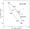 |
Fig. 1 Binary α Cen AB as it appears in the sky on various occasions. Shown is the orbit of α Cen B with respect to the primary A, which is at the origin, and with north up and east to the left. During the observing period, the separation of the stars was greatest in 2005 and smallest in 2011. The relative positions in the PACS (blue) and LABOCA (red) maps are indicated. The proper motion of α Cen for the time span between the LABOCA and PACS observations is shown by the dashed arrow. The separation between the stars at the time of the MIPS observations is indicated by the green dot. Orbital elements are adopted from Pourbaix et al. (2002). |
2. Observations and data reduction
2.1. Herschel
In the framework of our observing programme, i.e. the DUNES open time key programme, PACS photometric images were obtained at 100 μm and 160 μm. In addition, from the Hi-GAL survey (PI S. Molinari), we acquired archive data for α Cen at 70 μm and 160 μm obtained with PACS and at 250 μm, 350 μm, and 500 μm with SPIRE (Griffin et al. 2010). The relative position of the stars in the sky during the observational period is shown in Fig. 1.
2.1.1. DUNES: PACS 100 μm and 160 μm
PACS scan maps of α Cen were obtained at 100 μm and 160 μm at two array orientations (70° and 110°) to suppress detector striping. The selected scan speed was the intermediate setting, i.e. 20′′ s-1, determining the PSF at the two wavelengths (77 and 12′′, respectively). The 100 μm filter spans the region 85–130 μm and the 160 μm filter 130–210 μm and the observations at 100 and 160 μm were made simultaneously. The data were reduced with HIPE v.8.0.1. The native pixel sizes are 32 and 64 at 100 and 160 μm, respectively, and in the reduced images the resampling resulted in square pixels of 1′′ at 100 μm and 2′′ at 160 μm.
The two stellar components are approximated by model instrument PSFs of the appropriate wavelength based on an observation of α Boo rotated to match the telescope position angle of the α Cen observations. It is important to match the orientation of the PSF due to the non-circular tri-lobal structure of the Herschel-PACS PSF, which exists below the 10% peak flux level.
Fitting of the two components was carried out by subtracting the components in series, starting with the brighter one. Each component model PSF was scaled to the estimated peak brightness and shifted to the required positional offset from the observed source peak before subtraction. The position offset of B relative to A was fixed.
As described in detail by Eiroa et al. (2013), the level of the background and the rms sky noise were estimated by calculating the mean and standard deviation of 25 boxes sized 9′′ × 9′′ at 100 μm and 14′′ × 14′′at 160 μm scattered randomly at positions lying between 30′′–60′′ from the image centre and within the area of which no pixel was brighter than twice the standard deviation of all non-zero pixels in the image (the threshold criterion for source/non-source determination while high pass filtering during map creation). The calibration uncertainty was assumed to be 5% for both 100 μm and 160 μm (Balog et al. 2013)1.
Aperture (and potential colour) corrections of the stellar flux densities and sky noise corrections for correlated noise in the super-sampled images are described in the technical notes PICC-ME-TN-037 and PICC-ME-TN-038 and the NHSC/PACS home page2.
2.1.2. Hi-GAL: PACS 70 μm and 160 μm
As part of the Hi-GAL program, these data were obtained at a different scan speeds, i.e. the fast mode at 60′′ s-1. The field 314_0, containing α Centauri, was observed at both wavelengths simultaneously and in parallel with the SPIRE instrument (see next section). The scanned area subtends 2° × 2° and these archive data are reduced to Level 2.5. Compared to the data at longer wavelengths, background problems are much less severe at 70 μm. The PACS 70 μm data provide the highest angular resolution of all data presented here (Table 1). As before, no further colour correction was required, but the proper aperture correction (1.22) was applied. After re-binning, the pixel size is the same as that at 100 μm, viz. one square arcsecond, whereas the 160 μm pixels are, as before, two arcseconds squared.
Photometry and FIR/flux densities of α Centauri.
2.1.3. Hi-GAL: SPIRE 250 μm, 350 μm, and 500 μm
At the relatively low resolution of the SPIRE observations, the strong and varying background close to α Cen presented a considerable challenge for the flux measurements. However, for wavelengths beyond 160 μm, the dust emission from the galactic background is expected to be in the Rayleigh-Jeans (RJ) regime, and the emissivity should remain reasonably constant. Therefore, when normalised to a specific feature, the background is expected to look essentially the same at all wavelengths, when disregarding the slight deterioration of the resolution due to the smearing at the longest wavelengths. The result of this procedure is shown in Fig. 4, where α Cen is represented by the scaled PSFs and the background-subtracted fluxes are reported in Table 2. Assuming 10–30% higher (lower) fluxes for α Cen results in depressions (excesses) at the stellar position, which are judged unrealistic. This should therefore provide a reasonable estimate of the accuracy of these measurements. The photometric calibration of SPIRE is described by Bendo et al. (2013).
2.2. APEX
The Atacama Pathfinder EXperiment (APEX) is a 12 m submillimetre (submm) telescope located at 5105 m altitude on the Llano de Chajnantor in Chile. According to the APEX home page3, the telescope pointing accuracy is 2′′ (rms). The general user facilities include four heterodyne receivers within the approximate frequency bands 200−1400 GHz and two bolometer arrays, centred at 345 GHz (870 μm) and 850 GHz (350 μm), respectively. We used LABOCA and SHeFI APEX-1 for the observations of α Centauri.
2.2.1. LABOCA 870 μm
The Large APEX BOlometer CAmera (LABOCA) is a submillimetre array mounted on the APEX telescope (Siringo et al. 2009). The operating wavelength is 870 μm centred on a 150 μm wide window (345 and 60 GHz, respectively). With separations of 36′′, the 295 bolometers yield a circular field of view of 11 4. The angular resolution is HPBW = 195 and the under-sampled array is filled during the observations with a spiral mapping method.
The mapping observations of α Cen were made during two runs, viz. on 10–13 November 2007, and on 19 September 2009. The data associated with the programmes 380.C-3044(A) and 384.C-1025(A) were retrieved from the ESO archive. Since this observing mode is rather inefficient for point sources, we performed additional test observations with the newly installed telescope wobbler on 20 May and 13–14 July 2011. While centring α Cen B on LABOCA channel 71, the chopping was done by a fixed ± 25′′ in east-west direction, which resulted in asymmetric sky-flux pickup in this confused field, and these data therefore had to be discarded.
The map data were reduced and calibrated using the software package CRUSH 2 developed by Attila Kovács4. The data have been smoothed with a Gaussian of HPBW = 13′′, resulting in an effective FWHM = 234. However, fluxes in Jy/beam are given for an FWHM = 195.
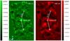 |
Fig. 2 Binary α Cen at 100 μm (left: green) and 160 μm (right: red) at high contrast. Scales are in Jy/pxl, where square pixels are 1′′ on a side at 100 μm and 2′′ on a side at 160 μm. The field of view is 1 |
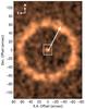 |
Fig. 3 Simulated observation at 160 μm of α Cen AB, assuming a face-on circumbinary dust disc/ring ( |


2.2.2. SHeFI 230 GHz (1300 μm)
Complementing observations were made with the Swedish Heterodyne Facility Instrument (SHeFI) APEX-1 during Director’s Discretionary Time (DDT) on 16 August 2012. APEX-1 is a single-sideband receiver that operates in the 230 GHz band (211–275 GHz) with an IF range of 4–8 GHz. At the CO (2–1) frequency, 230.5380 GHz, the half-power-beam-width is 27′′. The estimated main beam efficiency is ηmb = 0.75, and the kelvin-to-jansky conversion for the antenna is 39 Jy/K at this frequency.
The observing mode was on-the-fly (OTF) mapping with a scan speed of 6′′ s-1, which resulted in a data cube for the 5′ × 5′ spectral line map with 441 read-out points (Fig. 6). The reference, assumed free of CO emission, was at offset position (+ 1500′′, −7200′′). During the observations, the system noise temperature was typically Tsys = 200 K. As backend we used the fast Fourier transform spectrometer (FFTS) configured to 8192 channels having velocity resolution 0.16 km s-1, yielding a total Doppler bandwidth of 1300 km s-1.
These ON-OFF observations generate a data cube with two spatial dimensions (the “map”) and one spectral dimension (intensity vs frequency spectrum). The data were reduced with the xs-package by P. Bergman5. This included standard, low order, base line fitting, and subtraction, yielding for each “pixel” a spectrum with the intensity given relative to the zero-kelvin level (see Fig. 6a).
3. Results
3.1. Herschel PACS and SPIRE
The stars were clearly detected at both PACS 100 μm and 160 μm, as expected on the basis of the adopted observing philosophy of the DUNES programme. The last entry in Table 1 refers to the difference between the commanded position, corrected for proper and orbital motion, and the observed position, determined from the fitting of Gaussians to the data, and these are found to clearly be less than 2′′. This compares very favourably with the findings for PACS of the average offset of 24 by Eiroa et al. (2013) for a sample of more than 100 solar type stars. Similarly, observed offsets are also acceptable for the LABOCA data, i.e. within 2σ of the claimed pointing accuracy (Table 1).
Observed flux densities of α Cen A and B are given in Table 2, where the quoted errors are statistical and only refer to relative measurement accuracy. Absolute calibration uncertainties are provided by the respective instrument teams and cited here in the text. Together with complementing Spitzer MIPS data, these data are displayed in Fig. 7. For both α Cen A and B, a marginal excess at 24 μm corresponding to 2.5σ and 2.6σ is determined, respectively. The measured flux ratio at this wavelength corresponds well with the model ratio, i.e. 2.26 ± 0.11 and 2.25 respectively.
α Cen was detected at all SPIRE wavelengths, but with a marginal result at 500 μm (Fig. 5 and Table 2). As is also evident from these images, the pair was not resolved.
3.2. APEX LABOCA
The LABOCA fields are significantly larger than those of the PACS frames, and they contain a number of mostly extended sources of low intensity. However, α Cen is clearly detected (Fig. 5), but the binary components are not resolved. In Table 2, only the average is given for the 2007 and 2009 observations, because these flux densities are the same within the errors.
The proximity of the α Cen system leads to angular size scales that are rarely ever encountered among debris discs, which are generally much farther away. The PACS field of view is 105′′ × 210′′, so that a Edgeworth-Kuiper belt analogue would easily fill the images. The LABOCA frames contain structures similar to those discernable in Fig. 2. Although at faint levels, most of these sources are definitely real, because they repeatedly show up in independent data sets at different wavelengths obtained with different instruments and at different times. Knotty, but seemingly coherent, arcs and ring-like features on arcmin scales mimic the morphology of belt features. If these features were associated with the α Cen stars, they should move in concert with them at relatively high speeds. At 870 μm, the strongest feature lies less than one arcminute southeast of α Cen and is barely detectable at 100 μm, but clearly revealed at 160 μm. Measurements of the sky positions for both this feature (“Bright Spot”) and α Cen are reported in Table 3. For the Bright Spot these differ by +12 in right ascension (RA) and +09 in declination (Dec.), which provides an estimate of the measurement error, i.e. ~1′′ for relatively bright and centrally condensed sources.
Owing to its high proper motion, these values are significantly higher for α Cen, viz. Δ RA = −68 and Δ Dec = +29, at position angle PA ~ 247°. Neglecting the 01 parallactic contribution, SIMBAD6 data for α Cen yield for the 1.856 yr observing period Δ RA = −67, Δ Dec = +13, and PA = 259°.
Similar results are obtained involving other features in the 870 μm images. This provides firm evidence that the inhomogenous background is stationary and an unlikely part of any circumbinary material around α CenAB. A few notes concerning the nature of this background are given in the next section.
Dual epoch position data with LABOCA.
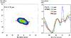 |
Fig. 4 Left: at 70 μm with PACS, the binary α Cen AB is clearly resolved (Hi-GAL data). As a result of the re-binning using cubic spline interpolation, the stars appear too close in this image. Right: the method for the estimation of the source and background fluxes in the SPIRE images is illustrated. Shown is a cut in right ascension through the image, normalised to the interstellar dust feature 40′′ east of α Cen. For comparison, the 160 μm PACS data are also shown in blue. For SPIRE, green identifies 250 μm, red 350 μm, and black 500 μm. |
3.3. APEX-1 SHeFI
In the direction of α Cen, strong CO (2–1) emission lines are found at local-standard-of-rest (LSR) velocities of −30, −50, and −60 km s-1, with a weaker component also at + 40 km s-1. This is entirely in accord with the observations of the Milky Way in CO (1–0) by Dame et al. (2001). As an example, the distribution of the integrated line intensity of the −50 km s-1 component is shown in Fig. 6, providing an overview of the molecular background in this part of the sky. With the line widths typical of giant molecular clouds, this confusing emission is certainly galactic in origin and not due to an anonymous IR-galaxy because the lines would be too narrow. We can also exclude the possibility of a hypothetical circumbinary dust disc around the pair α Cen AB, since the observed lines fall at unexpected LSR-velocities (υα Cen ~ − 3 km s-1) and are also too wide and too strong. Since these data do not reveal the continuum, the stars α Cen AB are not seen in the CO line maps.
4. Discussion
4.1. FIR and submm backgrounds
At a distance of 1.3 pc and located far below the ecliptic plane, any foreground confusion can be safely excluded. At greater distances, bright cirrus, dust emission from galactic molecular clouds, PDRs, H II regions, and/or background galaxies potentially contribute to source confusion at FIR and submm wavelengths. However, the projection of α Cen close to the galactic plane makes background issues rather tricky (see Sect. 2.1.3). In particular, extragalactic observers tend to avoid these regions, and reliable catalogues for IR galaxies are generally not available. However, as our spectral line maps show (Fig. 6), the observed patchy FIR/submm background is clearly dominated by galactic emission.
4.2. The SEDs of α Cen A and α Cen B
4.2.1. The stellar models
For the interpretation of the observational data we need to exploit reliable stellar atmosphere models and stellar physical parameters. The model photosphere parameters are based on the weighted average as the result of an extensive literature survey. The models have been computed by a 3D interpolation in a smoothed version of the high-resolution PHOENIX/GAIA grid (Brott & Hauschildt 2005) and with the following parameters from Torres et al. (2010) and the metallicities from Thévenin et al. (2002): (Teff, log g, [Fe/H]) = (5824 K, 4.3059, +0.195) for α Cen A and (5223 K, 4.5364, +0.231) for α Cen B. These models are shown in Fig. 7, together with the photometry (Table 2). We wish to point out again that these data have not been used in the analysis, but merely serve to illustrate the goodness of the models.
As a sanity check we compared the integrated model fluxes with the definition of the effective temperature, ∫ Sν dν/ ∫ Bν(Teff) dν. The luminosities are conserved to within 0.6% for α Cen A and 0.1% for α Cen B, which is well within the observational errors of 2% and 5%, respectively (Torres et al. 2010), which in turn are comparable to the errors of the theoretical model (e.g. Gustafsson et al. 2008; Edvardsson 2008). These small differences can probably be traced back to the re-gridding of the high-resolution models onto a somewhat sparser spectral grid.
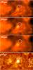 |
Fig. 5 Gallery of SPIRE and LABOCA data for α Centauri, which is inside the circles. Top to bottom: 250 μm, 350 μm, and 500 μm (SPIRE) and 870 μm (LABOCA), where the length of the arrow corresponds to 2′. |
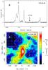 |
Fig. 6 a) Grand average of all CO (2–1) spectra, in Tmb vs. υLSR, of the 5′ × 5′ map toward α Centauri. Strong emission features at several lsr-velocities are evident in this direction of the Galaxy (ℓII = 315 |


4.2.2. The temperature minima of α Cen A and α Cen B
At heights of some five hundred kilometers above the visible photosphere (h ≲ 10-3 R⊙), the Sun exhibits a temperature minimum, i.e. T/Teff < 1, beyond which temperatures rise into the chromosphere and corona. Theories attempting to explain the physics of the heating of these outer atmospheric layers generally invoke magnetic fields (Carlsson & Stein 1995), but the details are far from understood and constitute an active field of solar research (e.g. de la Cruz Rodríguez et al. 2013). Such atmospheric structure can be expected to also be quite common on other and, in particular, solar-type stars. There, the dominating opacity, viz. H− free-free, limits the visibility to the FIR photosphere. For instance, on the Sun, Tmin occurs at wavelengths around 150 μm. This is very close to the spectral region, where this phenomenon has recently been directly measured for the first time also on another star (viz. α Cen A, Liseau et al. 2013), where in contrast to the Sun, the spatial averaging over the unresolved stellar disc is made directly by the observations. Since it is so similar in character, α Cen A may serve as a proxy for the Sun as a star (see also Pagano et al. 2004).
This Tmin-effect has also been statistically observed for a larger sample of solar-type stars (see Fig. 6 of Eiroa et al. 2013), a fact that could potentially contribute to enhancing the relationship between solar physics and the physics of other stars. In the end, such observations may help to resolve a long-standing puzzle in solar physics concerning the very existence of an actual gas temperature inversion at 500 km height and concerning whether this is occurring in the Quiet Sun or in active regions on the Sun (e.g., Leenaarts et al. 2011; Beck et al. 2013). Theoretical models have hitherto been inconclusive.
For α Cen A, Liseau et al. (2013) find that Tmin = 3920 ± 375 K, corresponding to the ratio Tmin/Teff = 0.67 ± 0.06. This is lower than observed for the Sun from spectral lines in the optical, viz. ~0.78 from analysis of the Ca ii K-line (Ayres et al. 1976). These authors also estimated this ratio for α Cen B, i.e. 0.71 and 0.72 using Teff = 5300 and 5150 K, respectively. For the data displayed in Fig. 7, we arrive at an estimate of Tmin = 3020 ± 850 K near 160 μm for this star. This results in Tmin/Teff = 0.58 ± 0.17, with Teff = 5223 ± 62 K. This value for α Cen B is slightly lower than the optically derived value, but the error on the infrared ratio is large. However, also for the Sun itself, Tmin determinations at different wavelengths show a wide spread of several hundred Kelvin (Avrett 2003).
In the present paper, we are however primarily concerned with the possible effects Tmin might have on estimation of very low emission levels from exo-Edgeworth-Kuiper belt dust. The intensity of the stellar model photosphere beyond 20 to 40 μm is commonly estimated from the extrapolation of the SED into the Rayleigh-Jeans (RJ) regime at the effective temperature Teff. There is a potential risk that this procedure will overestimate actual local stellar emissions, which may be suppressed at the lower radiation temperatures. In those cases where the SEDs are seemingly well fit by the RJ-extrapolations, the differences may in fact be due to emission from cold circumstellar dust (exo-Edgeworth-Kuiper belts), and here, we wish to quantify the magnitude of such an effect.
4.3. Far infrared: detectability of cool dust from Edgeworth-Kuiper belt analogues
The SED of α Cen A is exceptionally well-determined over a broad range of wavelengths, and we use it here for the estimation of the likely level of this effect on other, non-resolved systems. We do that by “filling the pit with sand” to determine the corresponding fractional dust luminosity fd ≡ Ldust/Lstar and the accompanying temperature of the hypothetical dust.
True Edgeworth-Kuiper belt analogues would be extremely faint and very difficult to detect (fd ⊙ ~ 10-7: Teplitz et al. 1999; Shannon & Wu 2011; Vitense et al. 2012). For estimating faint exo-Edgeworth-Kuiper belt levels, we apply simple dust ring models to “fill” the flux-dip of the temperature minimum of α Cen A, i.e. by minimising the chi-square for 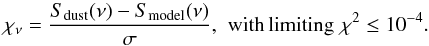 (1)For illustrative purposes, we place the object at a distance of 10 pc. Several ring temperatures were tested, and dust fluxes were adjusted to match the stellar RJ-SED. The modified black body of the dust was then adjusted to coincide with the difference in flux (i.e. stellar black body minus measured flux) at 160 μm and to a temperature that corresponds to the maximum of this flux difference.
This way of compensating for the Tmin-effect resulted in a dust temperature Tdust = 53 K at the modified black body radius of 34 AU and a formal fractional luminosity  , almost one order of magnitude below the detection limit of Herschel-PACS at 100 μm (fd ~ 10-6: see e.g. Fig. 1 of Eiroa et al. 2013) and comparable to what is estimated for the solar system Edgeworth-Kuiper belt (~10-7, Vitense et al. 2012). This fit is shown at the bottom of Fig. 8 where it is compared to the stellar SED and the difference between the black body and the temperature minimum fit, whereas the upper panel shows the observed data points, the adopted run of the Tmin-dip and that of the stellar RJ-SED.
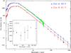 |
Fig. 7 SEDs of the binary α Cen AB. The model photospheres for the individual stars are shown by the blue and red lines. The PHOENIX model computations extend to about 45 μm (solid lines). At longer wavelengths, these correspond to extrapolations using the proper Bν(Teff) (dashes). Photometric data points are shown for comparison, with the upper limit being 3σ (Table 2). The green curve shows an ISO-SWS low-resolution observation, viz. TDT 60702006 (PI Waelkens; see also Decin et al. 2003). The inset displays the SED of the secondary α Cen B in the FIR/submm spectral region. |
Based on simple arguments, this dust temperature also provides a first-order estimate of the dust mass emitting at these wavelengths (cf. Hildebrand 1983), viz. ![Mathematical equation: \begin{equation} M_{\rm dust} \sim \frac { \left [ 1 - \frac{S_{\rm min}(\nu)}{S_{\rm model}(\nu)} \right ] S_{\rm model}(\nu)\,D^2 } { \kappa_{\rm ext}(\nu)\,B(\nu,\,T_{\rm dust}) }\cdot \label{mass} \end{equation}](/articles/aa/full_html/2014/03/aa21887-13/aa21887-13-eq153.png) (2)For an α Cen-like star not showing the Tmin effect, i.e. where the observed Sobs, min(ν) = Smodel(ν) (hence Mdust = 0), this formula would give a “concealed” dust mass of the order of the solar Edgeworth-Kuiper Belt (see e.g. Wyatt 2008), i.e. ≲10-3
(2)For an α Cen-like star not showing the Tmin effect, i.e. where the observed Sobs, min(ν) = Smodel(ν) (hence Mdust = 0), this formula would give a “concealed” dust mass of the order of the solar Edgeworth-Kuiper Belt (see e.g. Wyatt 2008), i.e. ≲10-3  for κ150 μm ≳ 10 cm2 g-1, depending on the largest size amax, the compactness and the degree of ice coating of the grains. For the cases considered here, reasonable values are within a factor of about 2 to 5 (e.g. Miyake & Nakagawa 1993; Krügel & Siebenmorgen 1994; Ossenkopf & Henning 1994). In general, κext(ν) = κsca(ν) + κabs(ν) is the frequency-dependent mass extinction coefficient. At long wavelengths, say λ > 5 μm, the scattering efficiency becomes negligible for the grains considered here, and κext reduces to κabs (κν henceforth).
In the FIR, i.e. for low frequencies, one customarily approximates the opacity by a power law, i.e. κν = κ0(ν/ν0) β when ν ≤ ν0, and where λ0 = c/ν0 > 2πa is a fiducial wavelength in the Rayleigh-Jeans regime, e.g. λ0 = 250 μm (Hildebrand 1983). For spherical Mie particles, the exponent of the frequency dependence of the emissivity β is in the interval 1 to 2 for most grain materials (Emerson 1988). For blackbody radiation, β = 0. For circumstellar dust, β-values around unity have commonly been found (e.g. Krügel & Siebenmorgen 1994; Beckwith et al. 2000; Wyatt 2008).
The rough estimate from Eq. (2) only refers to the a ≤ 1 mm regime and will thus not account for larger bodies, in many cases dominating the mass budget of debris discs (as in the solar system). As is commonly done in debris-disc studies, we distinguish between the dust mass and the total disc mass. To retrieve the mass of the unseen larger objects, numerical collisional models or analytical laws can be used (e.g. Thébault & Augereau 2007; Wyatt 2008; Löhne et al. 2008; Heng & Tremaine 2010a,b; Gáspár et al. 2012), but we focus here solely on the observable dust mass, which can be reasonably derived from infrared and subillimetre observations (Heng & Tremaine 2010a; Heng 2011). Even when obtained with an expression as simple as Eq. (2), these estimates are uncertain by at least a factor of several, because of uncertainties in the dust opacities.
From the dynamics of the binary system, we deduce (Appendix A) that a circumbinary disc is possible at a distance larger than 70−75 AU from the barycentre of the stars (see also Wiegert & Holman 1997; Jaime et al. 2012). Comparing the synthetic image of such a ring with an assumed outer radius of 105 AU in Fig. 3 with our observed continuum maps (Figs. 2 and 5), we find seemingly coherent structures at the proper distances of a face-on circumbinary ring. It is important to note that the circumbinary’s inclination may be unconstrained in contrast to the circumstellar discs that are dynamically limited to inclinations smaller than about 60°, (Wiegert & Holman 1997; see also Moutou et al. 2011 for a more general spin-orbit-inclination study). Also, Kennedy et al. (2012) report a circumbinary and circumpolar dust disc around 99 Herculis, which supports this possibility of non-coplanarity.
Regarding the possible detection of a circumbinary dust disc around α Cen AB, our single-epoch, multi-wavelength images would appear inconclusive. However, both proper motion and spectral line data obtained with APEX essentially rule out this scenario. If there is really a circumbinary disc or ring around α Centauri, it remained undetected by our observations.
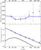 |
Fig. 8 Top: run of the brightness temperature of α Cen A, where the solid blue line is a fit through the data points around the temperature minimum, and the dashed blue line is the stellar blackbody extrapolation. The excess beyond 300 μm is presumed to originate in higher chromospheric layers (e.g. De la Luz et al. 2013). Bottom: SED of α Cen A scaled to the distance of 10 pc. The dashed black curve is the difference between the black body extrapolation (dashed blue line) and the Tmin-fit (solid blue line). The solid black curve is the emission of the fitted 53 K dust ring. |
4.4. Mid Infrared: warm zodi-dust in asteroid-like belts around α Cen A and α Cen B
4.4.1. Stable orbits
The tentative excesses at 24 μm may be due to warm dust. However, the binary nature of the α Cen system limits the existence of stable orbits to three possibilities. These are one large circumbinary disc with a certain inner radius and two circumstellar discs with maximum (or hereafter, critical) semi-major axes. These critical semi-major axes can be found using the semi-analytical expression of Holman & Wiegert (1999), viz.  (3)where e is the eccentricity of the binary orbit, μ = MB/(MA + MB) i.e. the fractional mass of the stars, aAB is the semi-major axis of the binary’s orbit, and the coefficients c1 through c6 (all with significant error bars) were computed by Holman & Wiegert (1999).
Using known parameters for α Cen (see Table 4), we can deduce that the circumstellar discs can not be larger than 2.78 ± 1.48 AU around α Cen A and 2.52 ± 1.60 AU around α Cen B, i.e. smaller than ~4 AU around either star (Table 4).
The putative Earth-mass planet, α Cen Bb (Dumusque et al. 2012) is small enough (~1.13 M⊕) that its Hill radius is just 4 × 10⁻⁴ AU. Our model discs never reach closer to the star than 0.08 AU, and consequently, this planet was neglected in our disc modelling.
Properties of the α Centauri binary.
Owing to the large errors of the estimated acrit, it was useful to test these limits with simple test-particle simulations of mass- and size-less particles. The resulting particle discs will also be used as a basis for radiative transfer simulations later. A steady state of these are shown in Fig. 9 where the accuracy of the Holman & Wiegert (1999) estimates is clear. Each simulation run was left for 103 orbital periods (i.e. ~8 × 10⁴ yr). The dynamics had earlier been examined also by others (e.g. Benest 1988; Wiegert & Holman 1997; Holman & Wiegert 1999; Lissauer et al. 2004; Thébault et al. 2009).
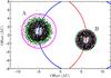 |
Fig. 9 Face-on circumstellar test-particle discs after ~ 103 periods shown with the stars close to periapsis. α Cen A is colour-coded blue (the left star and its orbit), and α Cen B is colour-coded red (the right star and its orbit). The green circles represent acrit around the stars and the magenta circles show estimates of their respective snow lines. |
These size limits are reminiscent of the inner solar system, i.e. this opens the possibility of an asteroid belt analogue for each star that forms dust discs through the grinding of asteroids and comets. Temperature estimates for the solar system zodiacal cloud are around 270 K and that of the fractional luminosity is about 10-7 (Fixsen & Dwek 2002; Nesvorný et al. 2010; Roberge et al. 2012), i.e. fd has a similar magnitude to the Edgeworth-Kuiper belt (Vitense et al. 2012).
4.4.2. Disc temperatures and snow lines
The Spitzer observations at 24 μm (PSF ≥ 6′′, Table 2; see also Kennedy et al. 2012) would not fully resolve these dynamically allowed discs. Strict lower temperature limits are provided by black body radiation from the discs, i.e. 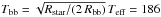 K and 147 K, respectively, for α Cen A and B, where the ratio of absorption to emission efficiency of unity for a black body has been used (e.g. Liseau et al. 2008; Lestrade et al. 2012; Heng & Malik 2013).
The α Cen circumstellar discs are constrained to radii smaller than 4 AU and should be relatively warm. We need to know, therefore, the locations of the snow lines in order to understand the likelihood of the presence of icy grains on stable orbits around these stars.
The snow line can be defined to be the largest radial distance at which the sublimation time scale is larger than all other relevant time scales of the system (Artymowicz 1997). Our estimations are based on the equations and methods by Grigorieva et al. (2007) and by Lamy (1974). The sublimation time was compared with the orbital time as a lower limit and the system age (4.85 × 10⁹ yr) as an upper limit. For the temperature-radius relation, we assumed blackbody emitters. This analysis resulted in sublimation temperatures between 154 K and 107 K for α Cen A, at the radial distances of 4.08 and 8.48 AU, respectively. Therefore, the snow line of α Cen A seems to be outside its dynamically stable region of 2.78 AU, which makes the presence of any icy disc grains not very likely (Fig. 9).
For α Cen B, sublimation temperatures were found to be between 157 K and 107 K, which corresponds to 2.23 and 4.81 AU, respectively. The lower bound is well inside the critical semi-major axis of 2.52 AU (see Fig. 9). Since this is based on an initial grain size of 1 mm (smaller sizes move the snow line outwards, while larger ones move it inwards), we can assume that the existence of a ring of larger icy grains and planetesimals is possible at the outer edge of the α Cen B disc. Such a ring could supply the disc with icy grains. However, these cannot be expected to survive in such a warm environment for long. Thus we assume that the iceless opacities from Miyake & Nakagawa (1993) are sufficient in this case. Ossenkopf & Henning (1994) have computed opacity models for the growth of ice coatings on grains. This conglomeration generally results in higher opacities than for their bare initial state.
We use dust opacities that are based on the models presented by Miyake & Nakagawa (1993), but scaled by a gas-to-dust mass ratio of one hundred. For a “standard” size distribution (Lestrade et al. 2012), i.e. n(a) ∝ a-3.5, the work by Ossenkopf & Henning (1994) gave similar results (see also e.g. Krügel & Siebenmorgen 1994; Stognienko et al. 1995; Beckwith et al. 2000). These works had different scopes, addressing specifically coagulation processes, rather than destructive collisions. However, for bare grains these opacites may also be applicable to some extent for the dust in debris discs7.
In the following sections we present synthetic SEDs obtained with the radiative transfer program RADMC-3D (Dullemond 2012) to assess the disc configurations in more detail.
4.5. Energy balance, temperature, and density distributions
Isothermal blackbody emission from thin rings would not make a realistic scenario for the emission from dust belts or discs. In particular, we need to specify the run of temperature and density, which is obtained from the solution to the energy equation, balancing the radiative heating with the cooling by the optically thin radiation.
In this balance equation, the loss term expresses the flux density of this thermal dust emission from an ensemble of grains received at the Earth, viz. 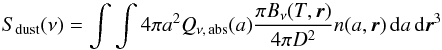 (4)where 4πa2Qν, abs(a) is the emissivity of the spherical grains with radius a, Qν, abs(a) is the absorption coefficient, n(a,r) is the volume density of the grains at location r, πBν is the thermal emittance at the equilibrium temperature T at r, and D is the distance to the source (so that 4πD2 ∫ Sdust(ν) dν = Ldust). The absorption coefficient Qν, abs is related to the dust opacity through Qν, abs = (4/3) κν ρ a, where ρ is the grain mass density, Qν, abs is shown as function of wavelength for a variety of materials and compositions for two grain sizes (10 and 1000 μm) in Fig. 4 of Krivov et al. (2013). We discuss grain sizes in the next section.
4.5.1. Grain size distribution
It is often assumed that n(a) ∝ a q describes the distribution in size of the grains (e.g. Miyake & Nakagawa 1993; Krügel & Siebenmorgen 1994; Ossenkopf & Henning 1994; Krivov et al. 2000). However, the shape, the existence, and magnitude of the power-law exponent q have been a matter of intense debate since Dohnanyi’s classic work on interplanetary particles in the solar system (Dohnanyi 1969). For a collision-dominated system at steady state, his result is summarised in a nutshell by the parameter s = 11/6, implying that q = 2 − 3s = −3.5 (see e.g. Dominik & Decin 2003; Wyatt 2008). This original work referred to the zodiacal cloud, but more recent estimates also for the much larger “grains”, i.e. Edgeworth-Kuiper belt objects (TNOs), by Bernstein et al. (2004) lead to a similar frequency spectrum for the diameters, dn/dD ∝ D− p and p = 4 ± 0.5, so that q = −3 ± 0.5 (see also Fraser & Kavelaars 2009).
More recent works have been following the collisional time evolution of dusty debris discs using numerical statistical codes. They have found rather strong deviations from true power laws, showing wiggles and wavy forms due to resonances (Krivov et al. 2006, 2013; Thébault & Augereau 2007; Löhne et al. 2008; Kral et al. 2013). However, mean values of these oscillations may still be consistent with power-law exponents that are not too dissimilar from the steady state Dohnanyi-distribution. In fact, Gáspár et al. (2012) find, from a large number of simulations, that q ~ − 3.65, i.e. slightly steeper than commonly assumed. Quoting Miyake & Nakagawa (1993), “q will be large (~−2.5) if the coagulation processes are dominant, whereas q will be small (~−3.5) if the disruption processes are dominant”, one might infer that disruptive collisions would dominate in debris discs, as expected. To be consistent with the exploited opacities, but also for comparison reasons, we are using a Dohnanyi distribution, i.e. n(a) ∝ a-3.5 that we use henceforth. For simplicity, the distribution of particle sizes in the disc is assumed to be homogeneous8 since the grains are large enough to not be significantly affected by drag forces and radiation pressure.
In Eq. (4), the integral over a extends over the finite range amin to amax, where we adopt for amax the upper bound for the κν-calculations, i.e. 1 mm. The smallest size, amin, is found for grains that are large enough not to be susceptible to the combined radiation pressure and stellar wind drag (Strubbe & Chiang 2006; Plavchan et al. 2009), i.e. ![Mathematical equation: \begin{equation} a_{\rm min} > a_{\rm blow} \approx \frac{ 3 } { 8\,\pi\,G\,M_{\rm star}\,\rho_{\rm grain} } \left [ \frac {L_{\rm star}} {c} + \dot{M}_{\rm star}\, \upsilon_{\rm w} \right ], \label{blowout} \end{equation}](/articles/aa/full_html/2014/03/aa21887-13/aa21887-13-eq243.png) (5)where we have set the radiative and wind coupling coefficients to unity for this order of magnitude estimate. Inside the brackets are the radiative and the mechanical momentum rates (“forces”), respectively. The stellar mass loss rate of α Cen A is close to that of the Sun, i.e. 2 × 10-14 M⊙ yr-1, and also the average wind velocity is similar, viz. υw ~ 400 km s-1 (Wood et al. 2001, 2005)9. This implies that the second term in Eq. (5) is negligible and that ablow = 0.64 μm for the stellar parameters of Table 4 and a grain density of 2.5 g cm-3 (for α Cen B, the corresponding a-value is about three times lower). It has been shown that the lower cut-off size is smooth (e.g. Wyatt et al. 2011; Löhne et al. 2012, and references therein) and up to about six times the blow-out radius, i.e. amin ~ 4 μm.
(5)where we have set the radiative and wind coupling coefficients to unity for this order of magnitude estimate. Inside the brackets are the radiative and the mechanical momentum rates (“forces”), respectively. The stellar mass loss rate of α Cen A is close to that of the Sun, i.e. 2 × 10-14 M⊙ yr-1, and also the average wind velocity is similar, viz. υw ~ 400 km s-1 (Wood et al. 2001, 2005)9. This implies that the second term in Eq. (5) is negligible and that ablow = 0.64 μm for the stellar parameters of Table 4 and a grain density of 2.5 g cm-3 (for α Cen B, the corresponding a-value is about three times lower). It has been shown that the lower cut-off size is smooth (e.g. Wyatt et al. 2011; Löhne et al. 2012, and references therein) and up to about six times the blow-out radius, i.e. amin ~ 4 μm.
In the next section, we calculate a number of numerical models for Eq. (4) by varying parameter values to get a feeling for how well (and uniquely) the observations can be reproduced. There were marginal excesses corresponding to 2.5σ at 24 μm for both α Cen A and α Cen B.
Model parameters for RADMC-3D disc calculations.
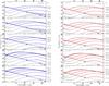 |
Fig. 10 Left: mid-infrared SEDs for α Cen A for different values of the power-law exponent q of the size distribution function, viz. n(a) ∝ a − q. Black curves depict dust SEDs, whereas blue curves display the total, i.e. |

4.5.2. RADMC-3D exozodi-disc calculations
RADMC-3D is a Monte-Carlo radiative transfer code, written primarily for continuum radiation through dusty media in an arbitrary three-dimensional geometry (developed by Dullemond 2012)10. It might seem an enormous “overkill” to use a radiative transfer program for the optically very thin discs discussed here, where the optical depth τ is comparable to the fractional luminosity fd of the dust disc. However, RADMC-3D is a convenient and user-friendly means to solve the energy equation, calculate SEDs, and convolve the model-images with the appropriate response functions of the used equipment for the observations (e.g. transmission curves, PSFs or beams, etc.). Details regarding the computational procedure can be found in Appendix A and examined parameters are presented in Table 5.
The basic input to RADMC-3D is a stellar model atmosphere (we use 3D interpolations in the PHOENIX/GAIA grid, Brott & Hauschildt 2005), a grid with dust densities for each included dust species, and absorption and scattering coefficients at each wavelength and for each dust species. The inner disc radii are given by the dust vaporation temperature11 of ~750 K and the outer radii determined by the binary dynamics. The discs have assumed height profiles h ~ 0.05 r β, with β = 0 (or β = 1; e.g., Wyatt 2008).
Also based on the dynamical model parameters are the dust mass estimations for various power- law exponents of the surface density, Σ ∝ r− γ, where γ ≥ 0. For reference, the solar minimum mass nebula (SMMN) has γ = 1.5 (Hayashi 1981). For the SMMN, at r0 = 1 AU, Σ0 ~ 2 × 10³ g cm-2, whereas exo-planet systems may have slightly steeper laws and somewhat higher Σ0 (Kuchner 2004).
Various grain size distributions were examined in accordance with Fig. 7 of Miyake & Nakagawa (1993), i.e. −4 ≤ q ≤ −2. The results of these computations are visualised in Fig. 10. There, we investigate whether any combination of parameters could be consistent with the observed data, i.e. the flux densities at 5, 24, and 70 μm. For α Cen A, acceptable models would imply values of fd ~ 10-5 for its hypothetical zodi, where q = −4 to −3.5. This would appear to agree with the result by Gáspár et al. (2012), i.e. q = −3.65.
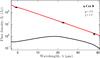 |
Fig. 11 Mid-infrared SED of α Cen B (star + dust, red curve) with data points. Assuming a “standard” disc model with q = 3.5 and γ = 1.5, the black curve shows the maximum emission from circumstellar dust that is consistent with the data. |
However, no such model was found that would fit the data for α Cen B, as illustrated in the right-hand panel of Fig. 10. These models assume a flat Σ-distribution, i.e. γ = 0. To be compatible with the observations, models for γ ≠ 0 would require very high values of γ (up to 10), making these “discs” more ring-like. However, best agreement was still achieved with γ = 0, when the model disc of α Cen B had less of an extent than the dynamically allowed size, i.e. Rin = 0.1 AU and Rout = 0.5 AU. The temperature profile is given by T(r) = 745 (r/0.05 AU)-0.55 K, and the dust-SED results in an fd = 3 × 10⁻⁵ for a dust mass  (3 × 10²⁰ g, i.e. about 10 − 30 mZ⊙) for grains with a = 4 μm to 1 mm and with sizes according to a q = −3.5 power law (see Fig. 11).
For both α Cen A and B, these limiting values of fd and md, respectively, would correspond to some 102 and 10 times those of the solar system zodi dust in ≲100 μm size particles (Roberge et al. 2012; Fixsen & Dwek 2002; Nesvorný et al. 2010). Fixsen & Dwek (2002) estimate the total mass of the asteroid belt at about  (2 × 1024 g). Heng & Tremaine (2010a,b) have calculated total disc masses for ages of about 3 Gyr. Their Fig. 7 would indicate that the mass of a “collision-limited” disc with a semi-major axis ≲4 AU and detected at 24 μm would amount to ~
 . In both cases, these estimations refer effectively to discs around single stars, and it is not entirely clear to what degree this also applies to multiple systems.
5. Conclusions
Based on FIR and submm photometric imaging observations from space (Herschel) and the ground (APEX) of α Cen, the following main conclusions can briefly be summarised as
-
Both binary components A and B were detected individually at 70 μm. At longer wavelengths, 100−870 μm, the pair was unresolved spatially during the time of observation, i.e. 8
4 in 2007 to 57 in 2011. -
At 100 and 160 μm, the solar twin α Cen A displays a temperature minimum in its SED, where the radiation originates at the bottom of its chromosphere. At longer wavelengths higher radiation temperatures are observed. This Tmin-effect is also marginally observed for α Cen B.
-
For solar-type stars not displaying the Tmin-phenomenon, compensating for the “missing flux” by radiation from optically thin dust could account for fractional dust luminosities, fd ~ 2 × 10⁻⁷, comparable to that of the solar system Edgeworth-Kuiper belt;
-
Combining Herschel data with mid-infrared observations (Spitzer) indicates marginal (2.5σ) excess emission at 24 μm in the SEDs of both stars. If caused by circumstellar emission from dust discs, fractional luminosity and dust mass levels would be some 10 to 100 times those of the solar zodiacal cloud.
The PACS calibration scheme is described further in detail at http://herschel.esac.esa.int/twiki/bin/view/Public/PacsCalibrationWeb#PACS_instrument_and_calibration
See also the homepage of B. Draine: http://www.astro.princeton.edu/~draine/dust/dustmix.html
In general, grain sizes may not be homogeneously distributed throughout circumstellar discs. Smaller grains may be more abundant in the outer parts of the discs and may even reside in the dynamical unstable regions in a binary, owing to production through collisions and radiation pressure (e.g. Thébault et al. 2010).
In this work the binary is not resolved into its components A and B, so that the quoted values refer to both of them. Athough α Cen B is the more active star of the two, we simply assumed equal mass loss rates.
This corresponds approximately to the low-density extrapolation of the data for olivine given by Pollack et al. (1994).
Acknowledgments
We thank the referee for the critical reading of the manuscript and the valuable suggestions that improved the quality of the paper. We are also grateful to H. Olofsson for granting his Director’s Discretionary Time to this project. We also wish to thank P. Bergman for his help with the APEX observations on such short notice and the swift reduction of the data. We appreciate the continued support of the Swedish National Space Board (SNSB) for our Herschel projects. The Swedish authors appreciate the continued support from the Swedish National Space Board (SNSB) for our Herschel projects. C. Eiroa, J. P. Marshall, and B. Montesinos are partially supported by Spanish grant AYA 2011/26202. A. Bayo was co-funded under the Marie Curie Actions of the European Comission (FP7-COFUND). S. Ertel thanks the French National Research Agency (ANR) for financial support through contract ANR-2010 BLAN-0505-01 (EXOZODI).
References
- Artymowicz, P. 1997, Ann. Rev. Earth Planet. Sci., 25, 175 [NASA ADS] [CrossRef] [Google Scholar]
- Avrett, E. H. 2003, in Current Theoretical Models and Future High Resolution Solar Observations: Preparing for ATST, eds. A. A. Pevtsov, & H. Uitenbroek, ASP Conf. Ser., 286, 419 [Google Scholar]
- Ayres, T. R., Linsky, J. L., Rodgers, A. W., & Kurucz, R. L. 1976, ApJ, 210, 199 [NASA ADS] [CrossRef] [Google Scholar]
- Balog, Z., Müller, T., Nielbock, M., et al. 2013, Experimental Astronomy, DOI: 10.1007/s10686-013-9352-3 [Google Scholar]
- Beck, C., Rezaei, R., & Puschmann, K. G. 2013, A&A, 556, A127 [NASA ADS] [CrossRef] [EDP Sciences] [Google Scholar]
- Beckwith, S. V. W., Henning, T., & Nakagawa, Y. 2000, in Protostars and Planets IV (Tucson: Univ. of Arizona Press), 533 [Google Scholar]
- Bendo, G. J., Griffin, M. J., Bock, J. J., et al. 2013, MNRAS, 433, 3062 [NASA ADS] [CrossRef] [Google Scholar]
- Benest, D. 1988, A&A, 206, 143 [NASA ADS] [Google Scholar]
- Bernstein, G. M., Trilling, D. E., Allen, R. L., et al. 2004, AJ, 128, 1364 [NASA ADS] [CrossRef] [Google Scholar]
- Bessell, M. S. 1990, PASP, 102, 1181 [NASA ADS] [CrossRef] [Google Scholar]
- Bigot, L., Kervella, P., Thévenin, F., & Ségransan, D. 2006, A&A, 446, 635 [NASA ADS] [CrossRef] [EDP Sciences] [Google Scholar]
- Brott, I., & Hauschildt, P. H. 2005, in The Three-Dimensional Universe with Gaia, eds. C. Turon, K. S. O’Flaherty, & M. A. C. Perryman, ESA SP, 576, 565 [Google Scholar]
- Carlsson, M., & Stein, R. F. 1995, ApJ, 440, L29 [NASA ADS] [CrossRef] [Google Scholar]
- Dame, T. M., Hartmann, D., & Thaddeus, P. 2001, ApJ, 547, 792 [NASA ADS] [CrossRef] [Google Scholar]
- de la Cruz Rodríguez, J., De Pontieu, B., Carlsson, M., & Rouppe van der Voort, L. H. M. 2013, ApJ, 764, L11 [NASA ADS] [CrossRef] [Google Scholar]
- Dela Luz, V., Raulin, J.-P., & Lara, A. 2013, ApJ, 762, 84 [NASA ADS] [CrossRef] [Google Scholar]
- Decin, L., Vandenbussche, B., Waelkens, K., et al. 2003, A&A, 400, 695 [NASA ADS] [CrossRef] [EDP Sciences] [Google Scholar]
- Desidera, S., & Barbieri, M. 2007, A&A, 462, 345 [NASA ADS] [CrossRef] [EDP Sciences] [Google Scholar]
- Dohnanyi, J. S. 1969, J. Geophys. Res., 74, 2531 [NASA ADS] [CrossRef] [Google Scholar]
- Dominik, C., & Decin, G. 2003, ApJ, 598, 626 [NASA ADS] [CrossRef] [Google Scholar]
- Dullemond, C. P. 2012, Astrophysics Source Code Library, ascl: 1202.015 [Google Scholar]
- Dumusque, X., Pepe, F., Lovis, C., et al. 2012, Nature, 491, 207 [NASA ADS] [CrossRef] [PubMed] [Google Scholar]
- Edvardsson, B. 2008, Phys. Scr. T, 133, 014011 [NASA ADS] [CrossRef] [Google Scholar]
- Eiroa, C., Marshall, J. P., Mora, A., et al. 2011, A&A, 536, L4 [NASA ADS] [CrossRef] [EDP Sciences] [Google Scholar]
- Eiroa, C., Marshall, J. P., Mora, A., et al. 2013, A&A, 555, A11 [NASA ADS] [CrossRef] [EDP Sciences] [Google Scholar]
- Emerson, J. P. 1988, in NATO ASIC Proc. 241: Formation and Evolution of Low Mass Stars, eds. A. K. Dupree & M. T. V. T. Lago, 21 [Google Scholar]
- Endl, M., Kürster, M., Els, S., Hatzes, A. P., & Cochran, W. D. 2001, A&A, 374, 675 [NASA ADS] [CrossRef] [EDP Sciences] [Google Scholar]
- Engels, D., Sherwood, W. A., Wamsteker, W., & Schultz, G. V. 1981, A&AS, 45, 5 [NASA ADS] [Google Scholar]
- Fixsen, D. J., & Dwek, E. 2002, ApJ, 578, 1009 [NASA ADS] [CrossRef] [Google Scholar]
- Fraser, W. C., & Kavelaars, J. J. 2009, AJ, 137, 72 [NASA ADS] [CrossRef] [Google Scholar]
- Gáspár, A., Psaltis, D., Rieke, G. H., & Özel, F. 2012, ApJ, 754, 74 [NASA ADS] [CrossRef] [Google Scholar]
- Griffin, M. J., Abergel, A., Abreu, A., et al. 2010, A&A, 518, L3 [Google Scholar]
- Grigorieva, A., Thébault, P., Artymowicz, P., & Brandeker, A. 2007, A&A, 475, 755 [NASA ADS] [CrossRef] [EDP Sciences] [Google Scholar]
- Guedes, J. M., Rivera, E. J., Davis, E., et al. 2008, ApJ, 679, 1582 [NASA ADS] [CrossRef] [Google Scholar]
- Gustafson, B. A. S. 1994, Ann. Rev. Earth Planet. Sci., 22, 553 [Google Scholar]
- Gustafsson, B., Edvardsson, B., Eriksson, K., et al. 2008, A&A, 486, 951 [NASA ADS] [CrossRef] [EDP Sciences] [Google Scholar]
- Hatzes, A. P. 2013, ApJ, 770, 133 [NASA ADS] [CrossRef] [Google Scholar]
- Hayashi, C. 1981, Prog. Theor. Phys. Suppl., 70, 35 [NASA ADS] [CrossRef] [MathSciNet] [Google Scholar]
- Heng, K. 2011, MNRAS, 415, 3365 [NASA ADS] [CrossRef] [Google Scholar]
- Heng, K., & Malik, M. 2013, MNRAS, 432, 2562 [NASA ADS] [CrossRef] [Google Scholar]
- Heng, K., & Tremaine, S. 2010a, MNRAS, 405, 701 [NASA ADS] [Google Scholar]
- Heng, K., & Tremaine, S. 2010b, MNRAS, 401, 867 [NASA ADS] [CrossRef] [Google Scholar]
- Hildebrand, R. H. 1983, QJRAS, 24, 267 [NASA ADS] [Google Scholar]
- Holman, M. J., & Wiegert, P. A. 1999, AJ, 117, 621 [NASA ADS] [CrossRef] [Google Scholar]
- Jaime, L. G., Pichardo, B., & Aguilar, L. 2012, MNRAS, 427, 2723 [NASA ADS] [CrossRef] [Google Scholar]
- Kennedy, G. M., Wyatt, M. C., Sibthorpe, B., et al. 2012, MNRAS, 421, 2264 [NASA ADS] [CrossRef] [Google Scholar]
- Kervella, P., Thévenin, F., Ségransan, D., et al. 2003, A&A, 404, 1087 [NASA ADS] [CrossRef] [EDP Sciences] [Google Scholar]
- Kral, Q., Thébault, P., & Charnoz, S. 2013, A&A, 558, A121 [NASA ADS] [CrossRef] [EDP Sciences] [Google Scholar]
- Krivov, A. V., Mann, I., & Krivova, N. A. 2000, A&A, 362, 1127 [NASA ADS] [Google Scholar]
- Krivov, A. V., Löhne, T., & Sremčević, M. 2006, A&A, 455, 509 [NASA ADS] [CrossRef] [EDP Sciences] [Google Scholar]
- Krivov, A. V., Eiroa, C., Löhne, T., et al. 2013, ApJ, 772, 32 [NASA ADS] [CrossRef] [Google Scholar]
- Krügel, E., & Siebenmorgen, R. 1994, A&A, 288, 929 [NASA ADS] [Google Scholar]
- Kuchner, M. J. 2004, ApJ, 612, 1147 [NASA ADS] [CrossRef] [Google Scholar]
- Lamy, P. L. 1974, A&A, 35, 197 [NASA ADS] [Google Scholar]
- Leenaarts, J., Carlsson, M., Hansteen, V., & Gudiksen, B. V. 2011, A&A, 530, A124 [NASA ADS] [CrossRef] [EDP Sciences] [Google Scholar]
- Lestrade, J.-F., Matthews, B. C., Sibthorpe, B., et al. 2012, A&A, 548, A86 [NASA ADS] [CrossRef] [EDP Sciences] [Google Scholar]
- Liseau, R., Risacher, C., Brandeker, A., et al. 2008, A&A, 480, L47 [NASA ADS] [CrossRef] [EDP Sciences] [Google Scholar]
- Liseau, R., Montesinos, B., Olofsson, G., et al. 2013, A&A, 549, L7 [NASA ADS] [CrossRef] [EDP Sciences] [Google Scholar]
- Lissauer, J. J., Quintana, E. V., Chambers, J. E., Duncan, M. J., & Adams, F. C. 2004, in Rev. Mex. Astron. Astrofis. Conf. Ser. 22, eds. G. Garcia-Segura, G. Tenorio-Tagle, J. Franco, & H. W. Yorke, 99 [Google Scholar]
- Löhne, T., Krivov, A. V., & Rodmann, J. 2008, ApJ, 673, 1123 [NASA ADS] [CrossRef] [Google Scholar]
- Löhne, T., Augereau, J.-C., Ertel, S., et al. 2012, A&A, 537, A110 [NASA ADS] [CrossRef] [EDP Sciences] [Google Scholar]
- Maldonado, J., Eiroa, C., Villaver, E., Montesinos, B., & Mora, A. 2012, A&A, 541, A40 [NASA ADS] [CrossRef] [EDP Sciences] [Google Scholar]
- Marshall, J. P., Moro-Martín, A., Eiroa, C., et al. 2014, A&A, accepted [Google Scholar]
- Miyake, K., & Nakagawa, Y. 1993, Icarus, 106, 20 [NASA ADS] [CrossRef] [Google Scholar]
- Moutou, C., Díaz, R. F., Udry, S., et al. 2011, A&A, 533, A113 [NASA ADS] [CrossRef] [EDP Sciences] [Google Scholar]
- Nesvorný, D., Jenniskens, P., Levison, H. F., et al. 2010, ApJ, 713, 816 [NASA ADS] [CrossRef] [Google Scholar]
- Ossenkopf, V., & Henning, T. 1994, A&A, 291, 943 [NASA ADS] [Google Scholar]
- Paardekooper, S.-J., & Leinhardt, Z. M. 2010, MNRAS, 403, L64 [NASA ADS] [Google Scholar]
- Pagano, I., Linsky, J. L., Valenti, J., & Duncan, D. K. 2004, A&A, 415, 331 [NASA ADS] [CrossRef] [EDP Sciences] [Google Scholar]
- Pilbratt, G. L., Riedinger, J. R., Passvogel, T., et al. 2010, A&A, 518, L1 [CrossRef] [EDP Sciences] [Google Scholar]
- Plavchan, P., Werner, M. W., Chen, C. H., et al. 2009, ApJ, 698, 1068 [NASA ADS] [CrossRef] [Google Scholar]
- Poglitsch, A., Waelkens, C., Geis, N., et al. 2010, A&A, 518, L2 [NASA ADS] [CrossRef] [EDP Sciences] [Google Scholar]
- Pollack, J. B., Hollenbach, D., Beckwith, S., et al. 1994, ApJ, 421, 615 [NASA ADS] [CrossRef] [Google Scholar]
- Porto de Mello, G. F., Lyra, W., & Keller, G. R. 2008, A&A, 488, 653 [NASA ADS] [CrossRef] [EDP Sciences] [Google Scholar]
- Pourbaix, D., Nidever, D., McCarthy, C., et al. 2002, A&A, 386, 280 [NASA ADS] [CrossRef] [EDP Sciences] [Google Scholar]
- Roberge, A., Chen, C. H., Millan-Gabet, R., et al. 2012, PASP, 124, 799 [NASA ADS] [CrossRef] [Google Scholar]
- Robertson, H. P. 1937, MNRAS, 97, 423 [NASA ADS] [Google Scholar]
- Roell, T., Neuhäuser, R., Seifahrt, A., & Mugrauer, M. 2012, A&A, 542, A92 [NASA ADS] [CrossRef] [EDP Sciences] [Google Scholar]
- Shannon, A., & Wu, Y. 2011, ApJ, 739, 36 [NASA ADS] [CrossRef] [Google Scholar]
- Siringo, G., Kreysa, E., Kovács, A., et al. 2009, A&A, 497, 945 [NASA ADS] [CrossRef] [EDP Sciences] [Google Scholar]
- Söderhjelm, S. 1999, A&A, 341, 121 [Google Scholar]
- Stark, C. C., & Kuchner, M. J. 2008, ApJ, 686, 637 [NASA ADS] [CrossRef] [Google Scholar]
- Stognienko, R., Henning, T., & Ossenkopf, V. 1995, A&A, 296, 797 [NASA ADS] [Google Scholar]
- Strubbe, L. E., & Chiang, E. I. 2006, ApJ, 648, 652 [NASA ADS] [CrossRef] [Google Scholar]
- Teplitz, V. L., Stern, S. A., Anderson, J. D., et al. 1999, ApJ, 516, 425 [NASA ADS] [CrossRef] [Google Scholar]
- Thébault, P. 2011, Celest. Mech. Dyn. Astron., 111, 29 [NASA ADS] [CrossRef] [Google Scholar]
- Thébault, P., & Augereau, J.-C. 2007, A&A, 472, 169 [NASA ADS] [CrossRef] [EDP Sciences] [Google Scholar]
- Thébault, P., Marzari, F., & Scholl, H. 2009, MNRAS, 393, L21 [NASA ADS] [CrossRef] [Google Scholar]
- Thébault, P., Marzari, F., & Augereau, J.-C. 2010, A&A, 524, A13 [NASA ADS] [CrossRef] [EDP Sciences] [Google Scholar]
- Thévenin, F., Provost, J., Morel, P., et al. 2002, A&A, 392, L9 [NASA ADS] [CrossRef] [EDP Sciences] [Google Scholar]
- Torres, G., Andersen, J., & Giménez, A. 2010, A&ARv, 18, 67 [Google Scholar]
- Vitense, C., Krivov, A. V., Kobayashi, H., & Löhne, T. 2012, A&A, 540, A30 [NASA ADS] [CrossRef] [EDP Sciences] [Google Scholar]
- Wiegert, P. A., & Holman, M. J. 1997, AJ, 113, 1445 [NASA ADS] [CrossRef] [Google Scholar]
- Wood, B. E., Linsky, J. L., Müller, H.-R., & Zank, G. P. 2001, ApJ, 547, L49 [NASA ADS] [CrossRef] [Google Scholar]
- Wood, B. E., Müller, H.-R., Zank, G. P., Linsky, J. L., & Redfield, S. 2005, ApJ, 628, L143 [Google Scholar]
- Wyatt, M. C. 2008, A&ARv, 46, 339 [CrossRef] [Google Scholar]
- Wyatt, M. C., Clarke, C. J., & Booth, M. 2011, Celest. Mech. Dyn. Astron., 111, 1 [NASA ADS] [CrossRef] [Google Scholar]
- Xie, J.-W., Zhou, J.-L., & Ge, J. 2010, ApJ, 708, 1566 [NASA ADS] [CrossRef] [Google Scholar]
Appendix A: Orbital dynamics and disc modelling
The test particle simulations were done for two reasons: firstly, to assess the binary dynamics per se and, secondly, for the steady state results to be used as disc models for radiative transfer simulations.
The standard equation of motion for circumstellar dust grains (around a single star) sums up most of the physical processes a grain experiences and is written as (Robertson 1937; Stark & Kuchner 2008) 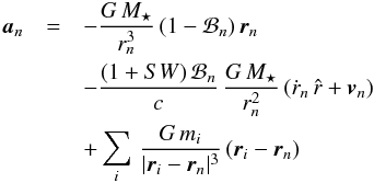 (A.1)for each test particle n. Here ℬn is the ratio between radiation pressure and gravitation exhibited on particle n, SW is the ratio between stellar-wind drag and Poynting-Robertson drag and is for the Sun about one third (~0.2–0.3, Gustafson 1994), and mi and ri are the mass and position of any planet in the system.
As hinted in Sect. 4.5.1, we consider grain sizes ≥4 μm. This is more than six times the blow-out radius, and consequently, we only solve the classical restricted three-body-problem, i.e. 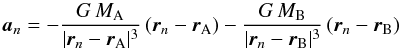 (A.2)for each test particle n. These simulations implemented a Runge-Kutta 4 integrator to solve the motions.
One particle disc was simulated at a time. The two circumstellar discs had identical initial conditions except for the central star; i.e., they had 104 particles in discs with constant particle density and radii smaller than 5 AU. The circumbinary disc also had constant particle density but was 100 AU in radius, (This was varied, but we only show results from the disc with 100 AU radius.) The circumbinary disc’s outer radius is, in contrast to the circumstellar discs, not constrained by the employed dynamics. Therefore the outer edge seen in Fig. 3 is artificial.
All discs were left to run for 103 periods, i.e. ~8 × 10⁴ yr, which was found to be sufficient to achieve a steady state. That the disc had settled by that time was verified with much longer runs (e.g. ~8 × 10⁵ yr). At the inner edge of the circumstellar discs, the grid resolution was up to 0.047 AU. On the much larger scale of the circumbinary disc, time steps of 0.1 yr were sufficient.
Finally, particles that came either closer than 0.001 Hill radii to each star or farther out than 1000 AU from the barycentre were removed. These limits were arbitrarily set on the basis of previous tests. The number of particles remaining varied from run to run with e.g. 2496 as the lowest (α Cen B with initial disc radius of 5 AU) up to 6717 (again α Cen B but with initial disc radius of 0.2 AU). The α Cen A disc with initial radius of 5 AU had 3538 remaining particles.
To compute dust SEDs, the dust disc density grid was obtained directly from the steady state discs. These were converted to a grid of mass densities with a large number of initially guessed dust masses, mdust. The proper temperature and density profiles yielded SEDs, which were compared to the data. The best fit was selected on the basis of its χ2-value.
All Tables
All Figures
|
Fig. 1 Binary α Cen AB as it appears in the sky on various occasions. Shown is the orbit of α Cen B with respect to the primary A, which is at the origin, and with north up and east to the left. During the observing period, the separation of the stars was greatest in 2005 and smallest in 2011. The relative positions in the PACS (blue) and LABOCA (red) maps are indicated. The proper motion of α Cen for the time span between the LABOCA and PACS observations is shown by the dashed arrow. The separation between the stars at the time of the MIPS observations is indicated by the green dot. Orbital elements are adopted from Pourbaix et al. (2002). |
| In the text | |
|
Fig. 2 Binary α Cen at 100 μm (left: green) and 160 μm (right: red) at high contrast. Scales are in Jy/pxl, where square pixels are 1′′ on a side at 100 μm and 2′′ on a side at 160 μm. The field of view is 1 |
| In the text | |
|
Fig. 3 Simulated observation at 160 μm of α Cen AB, assuming a face-on circumbinary dust disc/ring ( |
| In the text | |
|
Fig. 4 Left: at 70 μm with PACS, the binary α Cen AB is clearly resolved (Hi-GAL data). As a result of the re-binning using cubic spline interpolation, the stars appear too close in this image. Right: the method for the estimation of the source and background fluxes in the SPIRE images is illustrated. Shown is a cut in right ascension through the image, normalised to the interstellar dust feature 40′′ east of α Cen. For comparison, the 160 μm PACS data are also shown in blue. For SPIRE, green identifies 250 μm, red 350 μm, and black 500 μm. |
| In the text | |
|
Fig. 5 Gallery of SPIRE and LABOCA data for α Centauri, which is inside the circles. Top to bottom: 250 μm, 350 μm, and 500 μm (SPIRE) and 870 μm (LABOCA), where the length of the arrow corresponds to 2′. |
| In the text | |
|
Fig. 6 a) Grand average of all CO (2–1) spectra, in Tmb vs. υLSR, of the 5′ × 5′ map toward α Centauri. Strong emission features at several lsr-velocities are evident in this direction of the Galaxy (ℓII = 315 |
| In the text | |
|
Fig. 7 SEDs of the binary α Cen AB. The model photospheres for the individual stars are shown by the blue and red lines. The PHOENIX model computations extend to about 45 μm (solid lines). At longer wavelengths, these correspond to extrapolations using the proper Bν(Teff) (dashes). Photometric data points are shown for comparison, with the upper limit being 3σ (Table 2). The green curve shows an ISO-SWS low-resolution observation, viz. TDT 60702006 (PI Waelkens; see also Decin et al. 2003). The inset displays the SED of the secondary α Cen B in the FIR/submm spectral region. |
| In the text | |
|
Fig. 8 Top: run of the brightness temperature of α Cen A, where the solid blue line is a fit through the data points around the temperature minimum, and the dashed blue line is the stellar blackbody extrapolation. The excess beyond 300 μm is presumed to originate in higher chromospheric layers (e.g. De la Luz et al. 2013). Bottom: SED of α Cen A scaled to the distance of 10 pc. The dashed black curve is the difference between the black body extrapolation (dashed blue line) and the Tmin-fit (solid blue line). The solid black curve is the emission of the fitted 53 K dust ring. |
| In the text | |
|
Fig. 9 Face-on circumstellar test-particle discs after ~ 103 periods shown with the stars close to periapsis. α Cen A is colour-coded blue (the left star and its orbit), and α Cen B is colour-coded red (the right star and its orbit). The green circles represent acrit around the stars and the magenta circles show estimates of their respective snow lines. |
| In the text | |
|
Fig. 10 Left: mid-infrared SEDs for α Cen A for different values of the power-law exponent q of the size distribution function, viz. n(a) ∝ a − q. Black curves depict dust SEDs, whereas blue curves display the total, i.e. |
| In the text | |
|
Fig. 11 Mid-infrared SED of α Cen B (star + dust, red curve) with data points. Assuming a “standard” disc model with q = 3.5 and γ = 1.5, the black curve shows the maximum emission from circumstellar dust that is consistent with the data. |
| In the text | |
Current usage metrics show cumulative count of Article Views (full-text article views including HTML views, PDF and ePub downloads, according to the available data) and Abstracts Views on Vision4Press platform.
Data correspond to usage on the plateform after 2015. The current usage metrics is available 48-96 hours after online publication and is updated daily on week days.
Initial download of the metrics may take a while.