| Issue |
A&A
Volume 563, March 2014
|
|
|---|---|---|
| Article Number | A12 | |
| Number of page(s) | 9 | |
| Section | The Sun | |
| DOI | https://doi.org/10.1051/0004-6361/201220542 | |
| Published online | 26 February 2014 | |
Standing sausage waves in photospheric magnetic waveguides
1
Slovak Central Observatory,
PO Box 42,
94701
Hurbanovo,
Slovak Republic
e-mail:
ivan.dorotovic@suh.sk
2
Solar Physics & Space Plasma Research Centre
(SP 2RC),
School of Mathematics and Statistics, University of Sheffield,
Hicks Building, Hounsfield
Road, Sheffield,
S3 7RH,
UK
e-mail: robertus@sheffield.ac.uk; n.freij@sheffield.ac.uk
3
Hlohovec Observatory and Planetarium, Sládkovičova 41, 92001
Hlohovec, Slovak
Republic
e-mail:
astrokar@hl.cora.sk
4
Instituto de Astrofísica de Canarias, 38205, La Laguna, Tenerife, Spain
e-mail:
imarquez@ull.es
Received: 11 October 2012
Accepted: 4 December 2013
Aims. By focussing on the oscillations of the cross-sectional area and the total intensity of magnetic waveguides located in the lower solar atmosphere, we aim to detect and identify magnetohydrodynamic (MHD) sausage waves.
Methods. Capturing several high-resolution time series of magnetic waveguides and employing a wavelet analysis, in conjunction with empirical mode decomposition (EMD), makes the MHD wave analysis possible. For this paper, two sunspots and one pore (with a light bridge) were chosen as examples of MHD waveguides in the lower solar atmosphere.
Results. The waveguides display a range of periods from 4 to 65 min. These structures display in-phase behaviour between the area and intensity, presenting mounting evidence for sausage modes within these waveguides. The detected periods point towards standing oscillations.
Conclusions. The presence of fast and slow MHD sausage waves has been detected in three different magnetic waveguides in the solar photosphere. Furthermore, these oscillations are potentially standing harmonics supported in the waveguides that are sandwiched vertically between the temperature minimum in the lower solar atmosphere and the transition region. The relevance of standing harmonic oscillations is that their exploitation by means of solar magneto-seismology may allow insight into the sub-pixel resolution structure of photospheric MHD waveguides.
Key words: Sun: atmosphere / Sun: oscillations / sunspots / Sun: photosphere
© ESO, 2014
1. Introduction
Over the past decades, many oscillatory phenomena have been observed within a wide range of magnetic waveguides in the solar atmosphere (Banerjee et al. 2007; Wang 2011; Asai et al. 2012; Arregui et al. 2012). Sunspots and pores are just two of these many structures, and they are known to display solar global oscillations. See a recent review by, e.g., Pintér & Erdélyi (2011).
The commonly studied oscillatory periods in sunspots are three and five minutes. These oscillations are seen in intensity, line-of-sight (LOS) velocity, and LOS magnetic field. The source of the five-minute oscillation is a result of forcing by the five-minute (p-mode) global solar oscillation (Marsh & Walsh 2008), which forms the basis of helioseismology (Thompson 2006; Pintér & Erdélyi 2011). The five-minute oscillations are typically seen in simple molecular and non-ionized metal lines, which form low in the umbral photosphere and are moderately suppressed not only in the penumbra, but also in the chromospheric atmosphere above the umbra (Bogdan & Judge 2006). The cause of the three-minute oscillations is still unknown, but there are two main streams of theories. They could either be standing acoustic waves that are linked to the resonant modes of the sunspot cavity, or they could be low-β slow magneto-acoustic-gravity waves guided along the ambient magnetic field (Bogdan & Judge 2006). The three-minute oscillations are seen in plasma elements that form higher up and in the low chromosphere, and these are also moderately suppressed in the penumbra (Christopoulou et al. 2000).
When applied to a cylindrical magnetic flux tube, magnetohydrodynamic (MHD) theory reveals that a variety of waves can be supported, four of which are often reported in various structures in the solar atmosphere. Slow sausage (longitudinal) (De Moortel 2009; Wang 2011), fast kink (Andries et al. 2009a,b), fast sausage (McAteer et al. 2003), and Alfvén (torsional) waves (Jess et al. 2009), each affects the flux tube in a specific way. The sausage modes are of interest here, because the sausage mode is a compressible, symmetric perturbation around the axis of a flux tube that causes density perturbations that can be identified in intensity images (Fujimura & Tsuneta 2009). Furthermore, because the wave will either compress or expand the flux tube, the magnetic field will also show signs of oscillations. This mode may come in two forms in terms of phase speed classification: a slow mode (often also called the longitudinal mode), which generally has a phase speed close to the characteristic tube speed; and fast mode, which has a phase speed close to the external sound speed, assuming a region that has a plasma-β > 1 (Goossens 2003; Erdélyi 2008). A main difference between the two modes is the phase relationship between appropriate MHD quantities, which allows them to be identified. In this case, the fast sausage mode has an out-of-phase relationship between the area and intensity, while the slow sausage mode has an in-phase relationship. The technique that was applied to obtaining these phase relationships are covered by, say Goedbloed & Poedts (2004), Fujimura & Tsuneta (2009), Moreels & Van Doorsselaere (2013), and Moreels et al. (2013).
Sausage modes have been observed in solar pores. Dorotovič et al. (2008) observed a pore for 11 h and reported periodicities in the range of 20–70 min. These oscillations were consequently interpreted as linear low-frequency slow sausage waves. Morton et al. (2011) used the Rapid Oscillations in the Solar Atmosphere (ROSA) instrument to also identify linear sausage oscillations in a magnetic pore. However, determining whether the oscillations were slow or fast proved to be difficult. Morton et al. (2012), found the presence of fast sausage and kink waves higher in the solar atmosphere with enough wave energy to heat the chromosphere and corona.
The source and driving mechanism(s) of these MHD sausage modes have been very difficult to identify. Numerical simulations of a flux tube rooted in the photosphere, which is buffeted by a wide range of coherent sub-photospheric drivers, is one method for identifying the potential source of MHD sausage waves. These drivers can either be horizontal or vertical, single, or paired or else a power spectrum, with varying phase differences (see e.g. Malins & Erdélyi 2007; Khomenko et al. 2008; Fedun et al. 2011a,b; Vigeesh et al. 2012). One example of a horizontal driver is the absorption of the global solar p-mode oscillation by a sunspot (Goossens & Poedts 1992). More recently, Mathew (2008) has also studied this absorption and found a structured ring-like absorption pattern in Doppler power close to the umbral-penumbral boundary. This effect was strongest where the transverse magnetic field was at its greatest, and this region allows fast waves to be converted into slow magneto-acoustic waves, which are a potential source of MHD waves in sunspots and other similar magnetic structures.
We report observation of both slow and potentially fast sausage MHD waves in the lower solar atmosphere in three magnetic waveguides. In Sect. 2, we describe the data collection and the data processing method. In Sect. 3, we describe the results obtained from the three different data series and discuss our findings. Sect. 4 explains the underlying idea of identifying these oscillations as standing harmonics. Finally, in Sect. 5, we conclude.
2. Data collection and method of analysis
Three time series of images with high angular resolution have been chosen here in order to demonstrate the identification of MHD sausage waves. The images were taken in the G-band (430.5 nm), which samples the low photosphere. This line forms deep in the photosphere and has a line intensity defined as ρ2 × line-of-sight column depth.
The images were acquired using:
-
1.
The Swedish Vacuum Solar Telescope (SVST)situated on La Palma in the Canary Islands.Scharmer et al. (1985) pro-vides a detailed description of the features of the SVST.The images were taken on 7 July 1999.The sunspot is in the active region (AR)NOAA 8620. The observing duration is133 min with a cadence time of 25 s.The field of view (FOV) covers an area of33 600 km by 54[en-tity!#x2009!]600 km (1 pixel≈60 km). Bonet et al. (2005) gives a detailed analysis of this sunspot. A context image is the left-handed image of Fig. 1.
-
2.
The Dutch Open Telescope (DOT) is also situated on La Palma in the Canary Islands. Two series of imaging data sequences were taken using this telescope. A detailed guide of the features of the DOT is provided by Rutten et al. (2004). The first series of data were taken on 13 July 2005, and the sunspot is in the AR NOAA 10789. The region slowly decayed, and this sunspot led a small group of other magnetic structures. The observing length is 165 min and has a cadence time of 30 s. The second set of data, taken on 15 October 2008, is of one large pore with a light bridge which is about 15 pixels (750 km) wide in the AR NOAA 11005. The duration of the observing run is 66 min and has a cadence time of 20 s. Both DOT image sequences cover an area of 50 000 km by 45 000 km, where the maximum spatial resolution is 0.2′′ (≈140 km). Typical context images are the middle and right-handed panels of Fig. 1.
To obtain information relating to the cross-sectional area of these waveguides, a strict and consistent definition of the area is required. This definition is that each pixel with a value of less than 3σ of the median background intensity is counted as part of the waveguide. The background is defined as an area of the image where there are no formed magnetic structures. This may appear to be an arbitrary definition; however, a histogram of the background intensity reveals a Gaussian distribution, and when adding the area around and including the waveguide, there is significant peak on the lower end of the Gaussian distribution curve around 3σ or higher. Thus, we have a 99% confidence that the area is of the structure and not of the background.
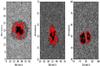 |
Fig. 1 An overview of the magnetic waveguides observed for this analysis. Left: the 1999 sunspot observed with the SVST with an average umbral area of 19 650 pixels (50 Mkm2). Middle: the 2005 sunspot observed with the DOT with an average umbral area of 12 943 pixels (32 Mkm2). Right: the 2008 pore observed with the DOT with an average area of 10 971 pixels (27 Mkm 2), the light bridge that separates the pore can be seen. Furthermore, these structures were seen near the disk centre, so there is little to no LOS effect. The red line shows the thresholding technique applied to each waveguide at the start of the data series. |
Figure 1 shows each waveguide at the start of the time series, where the red contour line represents the area found. The definition is accurate, but, it does include some non-waveguide pixels. The total intensity was determined by summing over the intensity of each pixel found in the waveguide. These waveguides are not static structures because, they slowly changed in size during the observing period. This background trend has to be removed for it not to mask any weak oscillation signatures. The detrending was accomplished by a non-linear regression fit and the consistency of the results was compared to subtracting the residue from an empirical mode decomposition (EMD) analysis (explained below). The residue is the data that remains after the EMD procedure has extracted as many signals as possible and it provides a very good approximation of the background trend.
The resulting reduced data series were then analysed with a wavelet tool in order to extract any periods of oscillation present within the data. The algorithm used is an adapted version of the IDL wavelet routine developed by Torrence & Compo (1998). The standard Morlet-wavelet, which is a plane sine wave with an amplitude modulated by a Gaussian function, was chosen for its suitable frequency resolution. The white cross-hatched area marks the cone of influence (COI), where edge effects of the wavelet structure affect the wavelet transform, and anything inside the COI is discarded. The white dashed line contour shows the confidence level of 95%. The wavelet method is very susceptible to noise at short periods and at times may not identify the true power of short periods.
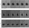 |
Fig. 2 Waveguides seen through six different parts of the observation sequence. The image sequence has time increasing from left to right. The first row is the 1999 sunspot, the middle row the 2005 sunspot, and the last row the 2008 pore. |
Beyond this, the data representing the size and intensity has also been analysed using EMD, which decomposes the time series into a finite number of intrinsic mode functions (IMFs). IMFs are essentially narrowband-filtered time series, with each IMF containing one or two periods that exist in the original data series. The EMD technique was first proposed by Huang et al. (1998) and offers some benefits over more traditional methods of analysis, such as wavelets or Fourier transforms. However, one drawback is that it is very prone to error with regards to long periods. For more information on the features and applicability of the EMD method, see e.g. Terradas et al. (2004). The problems associated with both the wavelet and EMD process means that the two complement each other. Furthermore, periods that appear in the wavelet just below the confidence level, but appear strongly in the EMD process, is a good indication that a period is not spurious. Generally, the next step after EMD analysis is to construct a Hilbert power spectrum that has a better time and spatial resolution than either wavelet or FFT routines. However, this has not been carried out owing to a lack of a robust code base at this time and will be addressed in future work. At this stage, we rely on wavelet and EMD analyses, as is customary in solar physics.
3. Results and discussion
3.1. LOS, circularity, and evolution of the waveguide
Several points need to be clarified for the data presented here before the full analysis. Firstly, there are LOS issues: Cooper et al. (2003a,b) have investigated how the LOS angle affects various aspects of observing coronal loops in a 2D model. Overall they found that for the slow sausage MHD wave, for a range of angles from π/6 to π/3, the observed intensity decreases as the LOS angle increases. Secondly, the larger angles lengthened the observed period of the wave. While the objects here are not coronal loops, the LOS angle still matters and should behave similarly. The LOS angles in all three cases were less than 30° thereby limiting any relevant effects of LOS.
Sunspots or pores are not fully circular and can have arbitrary shapes. The effects of a non-circular shape have been studied by, for example, Ruderman (2003), Morton & Erdélyi (2009), and Morton & Ruderman (2011). While they do not account for the very complicated and real structure of the sunspots and pores observed here, they still offer adequate insight. Current theory suggests the shape will have a minor effect on the oscillations unless it has a significant deviation from circularity. Likewise, the structure of each waveguide undergoes a minor change during the observation campaign, limiting any effects from large-scale structural change, as can be seen in Fig. 2.
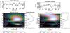 |
Fig. 3 Left image: evolution of the area of the 1999 sunspot (upper panel); the wavelet power spectrum for a white noise background, the cone of influence is marked as a cross-hatched area where edge effects become imporant and the contour lines show the 95% confidence level (lower left panel). Global (integrated in time) wavelet power spectrum, where the dashed line shows the 95% confidence limit (lower right panel). Right image: the same as the left image but for the mean intensity of the 1999 sunspot. |
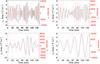 |
Fig. 4 The IMFs of the evolution of the area (red) and intensity (black) for the 1999 sunspot, over-plotted to aid comparison. Generally after the 6th IMF, higher IMFs lack a sufficient number of wave periods, which makes it difficult and less reliable to obtain an accurate period. |
3.2. MHD theory for phase relations
Treatment of the MHD equations makes it possible to determine phase relations between various physical quantities for propagating and standing MHD waves. This has been summarised briefly by Goedbloed & Poedts (2004) and also applied by Fujimura & Tsuneta (2009). The latter find that the phase relation for the slow MHD wave with regards to cross-sectional area and density is in phase regardless of whether the wave is propagating or standing. More recently, Moreels & Van Doorsselaere (2013) have expanded on this idea, taking factors into account such as LOS, which were neglected earlier, but also expanding the theory to cover fast MHD sausage waves. The phase relation for the magnetic field to the cross-sectional area is in phase when assuming that the plasma is frozen in to the magnetic field.
Supplementary information from other perturbation phase relations, such as velocity and the magnetic field, allows one to determine whether the observed MHD wave is slow or fast. In summary, the slow MHD sausage mode shows in-phase behaviour between intensity and area perturbations, while the fast sausage mode shows out-of-phase behaviour. Before progressing, we need to address the opacity effect on MHD wave perturbations. This is relevant, since intensity fluctuations can be due to the change of the optical depth along the LOS, which has the same phase difference as the fast MHD sausage wave and as a result is indistinguishable without further information (Fujimura & Tsuneta 2009).
Recently, Moreels et al. (2013) have analytically determined the phase difference between the cross-sectional area and the total intensity perturbations for both the slow and fast MHD sausage modes. They find that, for both the slow body and surface MHD wave, the behaviour is in phase, while for the fast surface wave, the behaviour is out of phase. This result means that it is possible to approximately separate slow and fast sausage waves without the use of other observable variables. Their results will be used here to distinguish between slow and fast MHD sausage modes.
3.3. Sunspot, 7 July 1999, AR 8620
Figure 3 shows the wavelet analysis of the 1999 sunspot area and intensity data. There are four confidently identified periods that exist in the area wavelet with 95% certainty; 4, 7, 16, and 32 min. The 32- min period is found over a wide range of the time series, with some of its power inside the COI. However, most is confidently outside the COI. The 16- min period is strongly localised at 50 to 120 min of the data series, starts at 18 min, and slowly increases and stabilises at 14 min. There is a third and fourth period at four and seven minutes that just reach the significance level and appear sporadically during the time series.
The intensity wavelet shows three distinct periods of oscillations above the confidence level: 4, 16, and 36.5 min. The 36.5-min period has a corresponding area wavelet oscillation at 32 min. While the 16-min oscillation corresponds to the 16-min oscillation found in the area. Furthermore, the 16-min period starts with very concentrated power and does not display the same period change as the area oscillation does. Finally, the four-minute period also corresponds to an oscillation found in the area but is also sporadic in its appearance.
It is safe to say that these oscillations are caused by sausage waves. The reason is that in linear ideal MHD theory, the sausage wave is the only MHD wave capable of changing the area of the flux tube that is observed on disk (see e.g. Cooper et al. 2003a; Wang 2004). Without the ability to directly compare the phase difference of the area to the intensity, great caution needs to be exercised to determine with confidence whether the perturbations are fast or slow. A wavelet phase diagram reveals regions (where the wavelet coherence is high and the period is ≤20 min) to be either out of phase or in phase, but a clear image of constant phase difference does not appear. This might be due to mode conversion occurring in the sunspot, since the G-band samples a region where the plasma-β≈1 in a magnetic structure (Gary 2001). When the period is ≥20 min, the only area of high coherence is located around 30 min and found to be nearly out-of-phase, which hints that there might be a fast surface sausage wave. However, only two full wave periods are outside the COI, which is due to the total length of the data series. This behaviour indicates that for short periods, a mixture of fast surface and slow MHD sausage waves are present while for the long period, it is purely a fast surface MHD sausage wave.
Figure 4 shows the computed IMFs for the 1999 sunspot data set. The IMFs show the periods of oscillations identified using the EMD routine. IMFs which show irrelevant periods, or the additional residue are ignored. In general, the higher order IMFs tend to show longer periods and, as such, contain fewer wave periods, which makes phase identification less reliable. Four IMF overlays are shown, and IMFs with similar periods to the wavelet plots have been overlaid in order to aid comparison for each dataset.
Four IMFs directly coincide with the wavelet period that reveal both area and intensity perturbations. IMF c3 displays the four-minute period where major regions of in-phase behaviour can be seen; however, either side shows one or two wave periods of out-of-phase behaviour. IMF c4 exhibits a period of seven minutes. The picture here is more muddled as an extra period is present in the intensity, namely 11 min, making phase identification harder for the seven-minute period. Where the IMFs coincide with the same period, namely at the start of the time series, the phase difference is approximately 45 degrees, which the authors have no theoretical explanation for. IMF c5 displays a 16-min period, with in-phase behaviour. Finally, IMF c6 contains the 32-min period. This period does not fully match the period seen in the intensity, but also one of the edge effects of the EMD process can be seen in the intensity signal. Near the end of the time series, the two IMFs overlap with the same period with an in-phase behaviour. In summary, the EMD process shows that the major behaviour is in phase, indicating the existence of a slow sausage mode. Also the regions of changing phase difference at lower periods indicates the potential existence of a fast surface mode. However, the last IMF does not agree with the wavelet phase due to the artefact from the EMD process.
It was possible to approximately separate the penumbra from the umbra and investigate its area for oscillations. However, the penumbra is a highly dynamic object and this makes the area estimation reasonably uncertain. There seem to be four periods that exist at 95% certainty: 5, 9, 15, and 25. The three shorter periods (5, 9, and 15 min) closely correspond to the 4-, 7-, and 16-min oscillations in the umbra; they could be a continuation of these umbral periods that became up-shifted as they enter the less compact structure of the penumbra. While the 25-min period does not directly correspond to an observed area oscillation. The wavelet phase analysis shows large regions of out-of-phase behaviour where the period is either below ten minutes or above 20 min. This behaviour is a mixed collection of fast surface and slow sausage modes, with regions moving from one phase difference to another after three or more wave periods.
3.4. Sunspot, 13 July 2005, AR 10789
Figure 5 shows the wavelet analysis of the 2005 sunspot area and intensity in AR 10789. There are four periods that exist at 95% confidence level: 4, 7.5, 11, and 16.5 min. Each period has a region of high power in the wavelet, with the lower periods appearing nearer the end of the time series. The corresponding intensity wavelet reveals that there are three periods of 4, 7.5, and 10.5 min oscillations; however, the 16.5-min oscillation is present but is a very weak signal. The cross-wavelet phase indicates that these oscillations are in phase. There are no major regions of out-of-phase behaviour.
Figure 6 shows the IMFs for the area and the intensity of the sunspot data in AR 10789. In this case, each period is found by the EMD process. IMF c2, IMF c3, IMF c4, and IMF c5 correspond to the 4, 7.5, 11, and 16.5-min oscillation periods, respectively. IMF c2 displays extensive in-phase behaviour throughout the time series, which is a strong indication of the slow sausage MHD wave at a period not too dissimilar to the global p-mode oscillation. The region of interest is within the time interval of 90 to 130 min for IMF c4, where the wavelet has these oscillations. The IMF shows clear in-phase behaviour in this time interval. The overall phase relation between the area and intensity indicates the presence of slow sausage waves.
3.5. Pore, 15 October 2008
Figure 7 shows the wavelet analysis of the pore with a light bridge. There are three periods that exist at 95% confidence level: 4.5, 8.5, and 14.5 min. The large part of the power of the period of 14–15 min is inside the COI; however, the period appears in the EMD analysis and has a large portion of power outside the COI and thus has not been ignored for this analysis. The three periods are seen in both area and intensity data when the wavelet analyses are cross-correlated. The power for these two periods is concentrated in the time interval of 20 to 60 min. The cross-wavelet analysis shows that the overlapping time span is somewhat smaller, at about 30 to 50 min. Furthermore, the wavelet power for each period runs parallel to each other throughout the time series, and they appear at the same time and seem to fade away at a similar time as well.
Figure 8 shows the IMFs for the area with intensity over-plotted. In this case, IMF c3 indicates a period of 4.5 min and IMF c4 has a characteristic period of 8.5 min, and this applies to both the area and intensity IMFs. IMF c3 reveals that the phase relation is in-phase for the majority of the time series. IMF c4 reveals large regions of roughly in-phase behaviour but with, again, a 45-degree phase difference. Not shown is the comparison of IMF c4 and IMF c5 for the area and intensity, respectively. At the end of the time series for both, there is a mixture of in-phase behaviour but also with the intensity signal leading the area signal for the 8.5 min oscillation. IMF c5 and IMF c6 for the area and intensity, respectively, show a period of 14.5 min. There is a region of near out-of-phase behaviour before this then turns into 45-degree phase difference with the area leading the intensity perturbations. Consistently, there are occurrences of unexplainable phase differences that require a theory to be developed to explain.
The easiest way to confirm the linearity of waves is to compare the amplitude of the oscillations to the characteristic scale of the structure. In all three cases studied here, the oscillation amplitudes are around 10% or less of the total area, which indicates that these oscillations are linear. Furthermore, the amplitude of the oscillation in the last two cases is by and large the same, so the amplitude has scaled with the size of the structure. However, for the 1999 sunspot, the amplitude of the oscillation is an order of a magnitude less. Whether this is due to the large size of the sunspot or the very stable nature during the observation window needs to be investigated in future work.
4. Standing harmonics
Basic MHD theory interpretation allows sunspots and pores to be described as vertical cylindrical flux tubes, with the base bounded in the photosphere and the top bounded at the transition region due to the sharp gradients in the plasma properties at these locations. Taking this further, an ideal flux tube is assumed here. The plasma density and magnetic field are homogeneous within the flux tube. This means that the standing harmonics of such flux tubes are the MHD equivalent to the harmonics in an open-ended compressible air pipe, where the ratio of the harmonic periods is given by P1/P2 = 2, P1/P3 = 3, and so forth. This only applies in the long-wavelength or thin-tube approximation. Using harmonic ratios to carry out magneto-seismology has been used, for example, by Andries et al. (2005a,b) who researched the effects of longitudinal density stratification on kink oscillations and resonantly damped kink oscillations, while Luna-Cardozo et al. (2012) studied longitudinal density effects and loop expansion on the slow sausage MHD wave. Luna-Cardozo et al. (2012) found that specific density profiles in lower atmospheric flux tubes could increase or decrease the value of the period ratio. The authors are unaware of any work that gives the changes to further harmonic ratios, so the assumption that the amount of deviation from the canonical value for the period ratio (P1/P2) is the same for other period ratios; e.g., P1/P3 or higher is used.
We now summarise the observed findings. Table 1 contains the periods of oscillations found in all three magnetic waveguides. There are four periods found for the 1999 sunspot. The second period of 16 min gives a period ratio (P1/P2) of 2 ± 0.2, which is exactly the same as the expected value of a uniform waveguide with a canonical value of 2. The next period ratio is 4.6 ± 0.3. Here, the change from canonical value is substantial if this is indeed the third period, which should be around 10.6 min, unless the effect on the harmonic ratio increases with each successive ratio. The last period is difficult to incorporate into the harmonic standpoint, and it is most likely that the four-minute period is due the global p-mode.
For the 2005 sunspot in AR 10789, there is a clearer picture of potential harmonics. The first period is 16.5 min and the second period is 11 min, which gives a ratio of 1.5 ± 0.2, and the third period of 7.5 min gives a ratio of 2.2 ± 0.3. The period ratio is modified downwards in a consistent manner as the harmonic number increases. These ratios are strong evidence of standing waves in this magnetic waveguide. As was the case for the 1999 sunspot, the period at four minutes has a period ratio that does not fit into this harmonic viewpoint and is most likely due to the global p-mode instead.
The periods of oscillations that are found in the area of the waveguides that exist at 95% confidence level.
For the 2008 pore of AR 11005, the picture is more muddled by the short available time series. Taking the 15-min period to be the first harmonic, the ratio is 1.7 ± 0.1 for the 8.5-min period, very similar to both first-period ratios of the previous sunspots. The third period is again very close to the period of the global p-mode.
The main conclusion to take away from this data analysis at this point is that the simple homogeneous flux tube model cannot fully account for these ratios. However, this simple model seems to be robust enough to give a good first insight. The most likely reasons for deviation from the canonical period ratio value are, firstly, that sunspots and pores (just like most lower atmospheric magnetic structures) expand with height, causing magnetic stratification (Verth & Erdélyi 2008; Luna-Cardozo et al. 2012), and secondly, that the Sun’s gravity causes density stratification (Andries et al. 2009b). These two effects will either increase or decrease the period ratio of the harmonics depending on the chosen density or magnetic profile (see Luna-Cardozo et al. 2012, for a detailed analysis in the context of slow sausage oscillations or see Erdélyi et al. 2013, for kink modes). In addition, these magnetic structures are rarely purely cylindrical, but can be elliptical (or arbitrary) in shape (see Ruderman & Erdélyi 2009; Morton & Erdélyi 2009) and in most cases are non-axially symmetric. Also, in some cases the flux tube is more suitably described as closed-ended at the photosphere and open-ended at the transition region, which would remove the even harmonics.
5. Conclusions
In this paper we have investigated three magnetic waveguides with the objective of detecting MHD sausage waves and determining whether they are slow or fast, propagating or standing. Based on the results presented here, we confidently interpreted the observed periodic changes in the area cross section of flux tubes, which are manifested as a pore and two sunspot waveguide structures, as proof of the existence of linear slow and fast surface sausage MHD oscillations. Using wavelet analysis, we found standing waves in the photosphere with periods ranging from 4 to 32 min. Employing complementary EMD analysis has allowed the detected MHD modes to be identified as a combination of fast surface sausage and slow sausage modes, thanks to the phase difference of the area and intensity. It is very likely that these oscillations are standing harmonics supported in a flux tube. The period ratio (P1/Pi = 2,3) of these oscillations indicates strongly that they are part of a group of standing harmonics in a flux tube that is non-homogeneous and bound by the photosphere and the transition region. Furthermore, there is possible indirect evidence of mode conversion occurring in one of these magnetic waveguides.
Acknowledgments
The authors thank J. Terradas for providing the EMD routine used in the data analysis and acknowledge M. Moreels for his theoretical discussions on phase relations. The authors would also like to thank the unknown referee for the helpful and insightful comments and suggestions. R.E. acknowledges M. Kéray for patient encouragement and is also grateful to NSF, Hungary (OTKA, Ref. No K83133). This work is supported by the UK Science and Technology Facilities Council (STFC). Wavelet power spectra were calculated using a modified computing algorithms of wavelet transform, the original of which was developed and provided by C. Torrence and G. Compo, and is available at URL: http://paos.colorado.edu/research/wavelets/. The DOT is operated by Utrecht University (The Netherlands) at Observatorio del Roque de los Muchachos of the Instituto de Astrofísica de Canarias (Spain) funded by the Netherlands Organisation for Scientific Research NWO, The Netherlands Graduate School for Astronomy NOVA, and SOZOU. The DOT efforts are part of the European Solar Magnetism Network. The SVST was operated by the Institute for Solar Physics, Stockholm, at the Observatorio del Roque de los Muchachos of the Instituto de Astrofísica de Canarias (La Palma, Spain).
References
- Andries, J., Arregui, I., & Goossens, M. 2005a, ApJ, 624, L57 [NASA ADS] [CrossRef] [Google Scholar]
- Andries, J., Goossens, M., Hollweg, J. V., Arregui, I., & Van Doorsselaere, T. 2005b, A&A, 430, 1109 [NASA ADS] [CrossRef] [EDP Sciences] [Google Scholar]
- Andries, J., Arregui, I., & Goossens, M. 2009a, A&A, 497, 265 [NASA ADS] [CrossRef] [EDP Sciences] [Google Scholar]
- Andries, J., van Doorsselaere, T., Roberts, B., et al. 2009b, Space Sci. Rev., 149, 3 [NASA ADS] [CrossRef] [Google Scholar]
- Arregui, I., Oliver, R., & Ballester, J. L. 2012, Liv. Rev. Sol. Phys., 9, 2 [Google Scholar]
- Asai, A., Ishii, T. T., Isobe, H., et al. 2012, ApJ, 745, L18 [NASA ADS] [CrossRef] [Google Scholar]
- Banerjee, D., Erdélyi, R., Oliver, R., & OShea, E. 2007, Sol. Phys., 246, 3 [NASA ADS] [CrossRef] [Google Scholar]
- Bogdan, T. J., & Judge, P. 2006, Phil. Trans. R. Soc. London, Ser. A, 364, 313 [Google Scholar]
- Bonet, J., Márquez, I., Muller, R., Sobotka, M., & Roudier, T. 2005, A&A, 430, 1089 [NASA ADS] [CrossRef] [EDP Sciences] [Google Scholar]
- Christopoulou, E. B., Georgakilas, A. A., & Koutchmy, S. 2000, A&A, 354, 305 [NASA ADS] [Google Scholar]
- Cooper, F. C., Nakariakov, V. M., & Tsiklauri, D. 2003a, A&A, 397, 765 [NASA ADS] [CrossRef] [EDP Sciences] [Google Scholar]
- Cooper, F. C., Nakariakov, V. M., & Williams, D. R. 2003b, A&A, 409, 325 [NASA ADS] [CrossRef] [EDP Sciences] [Google Scholar]
- De Moortel, I. 2009, Space Sci. Rev., 149, 65 [NASA ADS] [CrossRef] [Google Scholar]
- Dorotovič, I., Erdélyi, R., & Karlovský, V. 2008, eds. R. Erdélyi, & C. A. Mendoza-Briceño (Cambridge University Press), Proc. IAU Symp. 247, 351 [Google Scholar]
- Erdélyi, R. 2008, in Physics Of The Sun And Its Atmosphere, eds. B. N. Dwivedi, & U. Narain (World Scientific Publishing) [Google Scholar]
- Erdélyi, R., Hague, A., & Nelson, C. J. 2013, Sol. Phys. [arXiv:1306.1051] [Google Scholar]
- Fedun, V., Shelyag, S., & Erdélyi, R. 2011a, ApJ, 727, 17 [NASA ADS] [CrossRef] [Google Scholar]
- Fedun, V., Shelyag, S., Verth, G., Mathioudakis, M., & Erdélyi, R. 2011b, Ann. Geophys., 29, 1029 [Google Scholar]
- Fujimura, D., & Tsuneta, S. 2009, ApJ, 702, 1443 [NASA ADS] [CrossRef] [Google Scholar]
- Gary, G. 2001, Sol. Phys., 203, 71 [NASA ADS] [CrossRef] [Google Scholar]
- Goedbloed, J. P., & Poedts, S. 2004, Principles of magnetohydrodynamics: With applications to laboratory and astrophysical plasmas (Cambridge Univ. Press) [Google Scholar]
- Goossens, M. 2003, An introduction to plasma astrophysics and magnetohydrodynamics, Astrophys. Space Sci. Lib., 294 (Dordrecht: Kluwer Academic Publishers) [Google Scholar]
- Goossens, M., & Poedts, S. 1992, ApJ, 384, 348 [NASA ADS] [CrossRef] [Google Scholar]
- Huang, N., Shen, Z., Long, S., et al. 1998, Proc. R. Soc. A, 454, 903 [NASA ADS] [CrossRef] [Google Scholar]
- Jess, D., Mathioudakis, M., Erdélyi, R., et al. 2009, Science, 323, 1582 [NASA ADS] [CrossRef] [PubMed] [Google Scholar]
- Khomenko, E., Collados, M., & Felipe, T. 2008, Sol. Phys., 251, 589 [NASA ADS] [CrossRef] [Google Scholar]
- Luna-Cardozo, C., Verth, G., & Erdélyi, R. 2012, ApJ, 748, 110 [NASA ADS] [CrossRef] [Google Scholar]
- Malins, C., & Erdélyi, R. 2007, Sol. Phys., 246, 41 [NASA ADS] [CrossRef] [Google Scholar]
- Marsh, M. & Walsh, R. 2008, ApJ, 643, 540 [Google Scholar]
- Mathew, S. K. 2008, Sol. Phys., 251, 515 [NASA ADS] [CrossRef] [Google Scholar]
- McAteer, R., Gallagher, P., Williams, D., et al. 2003, ApJ, 587, 806 [NASA ADS] [CrossRef] [Google Scholar]
- Moreels, M., & Van Doorsselaere, T. 2013, A&A, 551, A137 [NASA ADS] [CrossRef] [EDP Sciences] [Google Scholar]
- Moreels, M. G., Goossens, M., & Van Doorsselaere, T. 2013, A&A, 555, A75 [NASA ADS] [CrossRef] [EDP Sciences] [Google Scholar]
- Morton, R. J., & Erdélyi, R. 2009, A&A, 502, 315 [NASA ADS] [CrossRef] [EDP Sciences] [Google Scholar]
- Morton, R. J., & Ruderman, M. S. 2011, A&A, 527, A53 [NASA ADS] [CrossRef] [EDP Sciences] [Google Scholar]
- Morton, R. J., Erdélyi, R., Jess, D. B., & Mathioudakis, M. 2011, ApJ, 729, L18 [NASA ADS] [CrossRef] [Google Scholar]
- Morton, R. J., Verth, G., Jess, D. B., et al. 2012, Nature Commun., 3, 1315 [Google Scholar]
- Pintér, B., & Erdélyi, R. 2011, Space Sci. Rev., 158, 471 [NASA ADS] [CrossRef] [Google Scholar]
- Ruderman, M. S. 2003, A&A, 409, 287 [NASA ADS] [CrossRef] [EDP Sciences] [Google Scholar]
- Ruderman, M. S., & Erdélyi, R. 2009, Space Sci. Rev., 149, 199 [NASA ADS] [CrossRef] [Google Scholar]
- Rutten, R., Hammerschlag, R., Bettonvil, F., Sütterlin, P., & De Wijn, A. 2004, A&A, 413, 1183 [NASA ADS] [CrossRef] [EDP Sciences] [Google Scholar]
- Scharmer, G., Brown, D., Pettersson, L., & Rehn, J. 1985, Appl. Opt., 24, 2558 [NASA ADS] [CrossRef] [Google Scholar]
- Terradas, J., Oliver, R., & Ballester, J. 2004, ApJ, 614, 435 [NASA ADS] [CrossRef] [Google Scholar]
- Thompson, M. J. 2006, Phil. Trans. R. Soc. London, Ser. A, 364, 297 [Google Scholar]
- Torrence, C. & Compo, G. 1998, Bull. Am. Meteorol. Soc., 79, 61 [Google Scholar]
- Verth, G., & Erdélyi, R. 2008, A&A, 486, 1015 [NASA ADS] [CrossRef] [EDP Sciences] [Google Scholar]
- Vigeesh, G., Fedun, V., Hasan, S., & Erdélyi, R. 2012, ApJ, 755, 18 [NASA ADS] [CrossRef] [Google Scholar]
- Wang, T. 2004, in SOHO 13 Waves, Oscillations and Small-Scale Transients Events in the Solar Atmosphere: Joint View from SOHO and TRACE, ESA SP-547, 417 [Google Scholar]
- Wang, T. 2011, Space Sci. Rev., 158, 397 [NASA ADS] [CrossRef] [Google Scholar]
All Tables
The periods of oscillations that are found in the area of the waveguides that exist at 95% confidence level.
All Figures
|
Fig. 1 An overview of the magnetic waveguides observed for this analysis. Left: the 1999 sunspot observed with the SVST with an average umbral area of 19 650 pixels (50 Mkm2). Middle: the 2005 sunspot observed with the DOT with an average umbral area of 12 943 pixels (32 Mkm2). Right: the 2008 pore observed with the DOT with an average area of 10 971 pixels (27 Mkm 2), the light bridge that separates the pore can be seen. Furthermore, these structures were seen near the disk centre, so there is little to no LOS effect. The red line shows the thresholding technique applied to each waveguide at the start of the data series. |
| In the text | |
|
Fig. 2 Waveguides seen through six different parts of the observation sequence. The image sequence has time increasing from left to right. The first row is the 1999 sunspot, the middle row the 2005 sunspot, and the last row the 2008 pore. |
| In the text | |
|
Fig. 3 Left image: evolution of the area of the 1999 sunspot (upper panel); the wavelet power spectrum for a white noise background, the cone of influence is marked as a cross-hatched area where edge effects become imporant and the contour lines show the 95% confidence level (lower left panel). Global (integrated in time) wavelet power spectrum, where the dashed line shows the 95% confidence limit (lower right panel). Right image: the same as the left image but for the mean intensity of the 1999 sunspot. |
| In the text | |
|
Fig. 4 The IMFs of the evolution of the area (red) and intensity (black) for the 1999 sunspot, over-plotted to aid comparison. Generally after the 6th IMF, higher IMFs lack a sufficient number of wave periods, which makes it difficult and less reliable to obtain an accurate period. |
| In the text | |
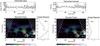 |
Fig. 5 Same as Fig. 3 but for the sunspot in AR 10789 in 2005. |
| In the text | |
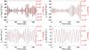 |
Fig. 6 Same as Fig. 4 but for the sunspot in AR 10789 in 2005. |
| In the text | |
 |
Fig. 7 Same as Fig. 3 but for the pore in AR 11005 in 2008. |
| In the text | |
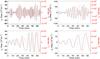 |
Fig. 8 Same as Fig. 4 but for the pore in AR 11005 in 2008. |
| In the text | |
Current usage metrics show cumulative count of Article Views (full-text article views including HTML views, PDF and ePub downloads, according to the available data) and Abstracts Views on Vision4Press platform.
Data correspond to usage on the plateform after 2015. The current usage metrics is available 48-96 hours after online publication and is updated daily on week days.
Initial download of the metrics may take a while.