| Issue |
A&A
Volume 562, February 2014
|
|
|---|---|---|
| Article Number | A134 | |
| Number of page(s) | 14 | |
| Section | Galactic structure, stellar clusters and populations | |
| DOI | https://doi.org/10.1051/0004-6361/201322617 | |
| Published online | 20 February 2014 | |
A lower bound on the Milky Way mass from general phase-space distribution function models⋆
1
Institute of Nuclear Physics, Polish Academy of Sciences,
Radzikowskego 152,
31342
Kraków,
Poland
e-mail:
This email address is being protected from spambots. You need JavaScript enabled to view it.
2
Astronomical Observatory, Jagiellonian University,
Orla 171,
30244
Kraków,
Poland
3
Institute of Physics, Jagiellonian University,
Reymonta 4,
30059
Kraków,
Poland
Received:
5
September
2013
Accepted:
4
December
2013
Abstract
We model the phase-space distribution of the kinematic tracers using general, smooth distribution functions to derive a conservative lower bound on the total mass within ≈150−200 kpc. By approximating the potential as Keplerian, the phase-space distribution can be simplified to that of a smooth distribution of energies and eccentricities. Our approach naturally allows for calculating moments of the distribution function, such as the radial profile of the orbital anisotropy. We systematically construct a family of phase-space functions with the resulting radial velocity dispersion overlapping with the one obtained using data on radial motions of distant kinematic tracers, while making no assumptions about the density of the tracers and the velocity anisotropy parameter β regarded as a function of the radial variable. While there is no apparent upper bound for the Milky Way mass, at least as long as only the radial motions are concerned, we find a sharp lower bound for the mass that is small. In particular, a mass value of 2.4 × 10¹¹ M⊙, obtained in the past for lower and intermediate radii, is still consistent with the dispersion profile at larger radii. Compared with much greater mass values in the literature, this result shows that determining the Milky Way mass is strongly model-dependent. We expect a similar reduction of mass estimates in models assuming more realistic mass profiles.
Key words: techniques: radial velocities / Galaxy: halo / Galaxy: kinematics and dynamics / Galaxy: fundamental parameters / methods: numerical
Full Table 1 is only available at the CDS via anonymous ftp to cdsarc.u-strasbg.fr (130.79.128.5) or via http://cdsarc.u-strasbg.fr/viz-bin/qcat?J/A+A/562/A134
© ESO, 2014
1. Introduction
The asymptotic value of galactic mass function (total mass) can be ascertained through studying the radial motions of distant kinematic tracers, which are regarded as test bodies moving under the influence of the galactic gravitational field. A primary quantity for describing a collection of these bodies is a phase-space distribution function (PDF) which must be non-negative everywhere. The function gives rise to various theoretical secondary quantities such as the radial velocity dispersion (RVD), the flattening of the velocity ellipsoid β (the anisotropy parameter), the number density of tracers, mean velocities, etc, which in general may be functions of space variables defined as appropriate integrals involving the PDF. On comparison with the corresponding quantities from measurements, the total mass can be inferred.
The accustomed approach to this technique of determining the total mass is based on Jeans modeling of a stationary collision-less system of identical bodies in a steady-state equilibrium1 (Jeans 1915). Jeans concludes his work by saying that the Galaxy has not yet reached a final steady state on account of the fact that such a state seems to be inconsistent with the observed streaming motions. The principal assumption of this technique requires that the kinematic tracers are relaxed in the gravitational potential and can be described in terms of a smooth PDF. However, the assumption of collision-less equilibrium may not necessarily be appropriate. In particular, this may be the case both for fast moving tracers (e.g., propelled by the three-body ejecting mechanism, which is collisional in its nature) and for most distant tracers, on orbits characterized by large time scales, which are likely to be influenced by the material distributed on larger scales in the Local Group. It is also doubtful that the very notion of a smooth distribution is applicable to an extremely rarefied collection of the outermost satellites of the Milky Way (MW). Although Jeans’ modeling is a powerful tool that was fruitful in many cases, it should be remembered that it has a limited application.
In recent years, there has been growing interest in the most general distributions functions that can be fit to dynamical data with most general and assumption-free constraints on the gravitational potential and mass profile. Under the assumption that a galaxy is in a steady state, Magorrian (2014) proposes a new framework of inferring the gravitational potential from a discrete realization of the unknown distribution function provided by the snapshots of a galaxy’s stellar kinematics. Bovy et al. (2010) used instantaneous kinematic snapshots of radial distances and velocities to infer the force law with a fully Bayesian inference technique. As an example, when applying it to the solar system, the correct exponent in the power form of the force law was almost precisely reconstructed, largely independent of the PDF of two variables (energy and eccentricity) with no need to make strong assumptions about the anisotropy. As noted in Bovy et al. (2010), generalizations of the methods used therein would permit inference of MW dynamics from upcoming surveys, such as the Gaia mission (Perryman et al. 2001), or of the mass of the central black hole.
In this paper, the form of PDF is also general. Its form is not assumed except that it should be a function of integrals of motion to automatically satisfy the Boltzmann equation. Our aim is to find, in a given gravitational potential that allows for such integrals, a variety of PDFs consistent with the radial distance-velocity data. In this preliminary work, we do not make any assumptions about the form of other secondary observables derivable from a given PDF (such as the transverse velocity dispersion or the profile of the anisotropy parameter) that could be used to constrain the variety of consistent PDFs. We focus instead on the resulting estimate of the MW’s minimum total mass.
The secondary quantities referred to above are not all independent. They are constrained to satisfy (moment) Jeans equations. However, satisfying them is not sufficient for the positivity of the PDF. In principle, having found a solution, the positivity condition should be checked separately. Jeans equations are usually underdetermined – there is arbitrariness in choosing solutions. Some of the secondary quantities must be assumed (along with the mass function of the host gravitational field). This makes the problem of determining the total mass model-dependent and biased by inescapable degeneracies. The existing mass estimates can differ largely between each other. The differences lie both on the side of choosing sample tracers and making model assumptions. In the context of this under-determinacy, one cannot exclude that masses predicted by various models can be overestimated. The mechanism of this overestimation can be understood as follows. The total mass can be regarded as a functional defined on the space of solutions to the Jeans equation2. As said above, various quantities entering that equation must involve additional assumptions. These assumptions are introduced in the form of constraints, such as a constant value for β, a power law for the number density, and the particular form of the gravitating mass function of the host potential. These constraints impose some indirect restrictions on the PDF function. As for any functional with constraints, so also for the total mass functional, one can expect that the lower bound may be increased compared to that without constraints3.
From the above consideration, a natural question arises for the lower bound of the MW mass. This question motivates our paper. Our aim is to show that with a given set of radial motions of kinematic tracers, the estimated mass can be much lower than usually obtained in the literature. We postpone answering this question until Sects. 3 and 4.
Another, but related, question concerns the upper bound. It may be answered more
straightforwardly. We consider the point mass potential – the asymptotics of any physical
mass distribution. The time average  for a single
elliptical orbit with eccentricity e, suggests that
for a single
elliptical orbit with eccentricity e, suggests that
 for
almost circular orbits. Assuming this behavior of
for
almost circular orbits. Assuming this behavior of  in the spherical Jeans
equation
in the spherical Jeans
equation  , along with the
vanishing mean velocities, constant
, along with the
vanishing mean velocities, constant  ,
and
,
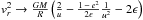
and  (ε > 0), we conclude that
asymptotically, when r Φ ~ − GM, the mass estimate for
almost circular orbits is
(ε > 0), we conclude that
asymptotically, when r Φ ~ − GM, the mass estimate for
almost circular orbits is  (1)This result holds
without the need for the phenomenological explicit assumption that
. A
general integral of the spherical Jeans equation found in An
& Evans (2009) under similar assumptions about β and ρ, reduces in the point mass
potential to
(1)This result holds
without the need for the phenomenological explicit assumption that
. A
general integral of the spherical Jeans equation found in An
& Evans (2009) under similar assumptions about β and ρ, reduces in the point mass
potential to  (in our
notational convention), where C is an integration constant. In the asymptotical
regime we work in, the appropriate boundary condition is to require that
should be finite in the limit
r → ∞, which
for 4−2β + ε > 0
implies that C = 0, again giving (1). Result (1) says that
an almost flat
(in our
notational convention), where C is an integration constant. In the asymptotical
regime we work in, the appropriate boundary condition is to require that
should be finite in the limit
r → ∞, which
for 4−2β + ε > 0
implies that C = 0, again giving (1). Result (1) says that
an almost flat  profile could be explained by
arbitrary large M (β and ε are not controlled by measurements at large
radii4). There is no apparent upper bound for the
mass. This will become even more evident in Sect. 4.
profile could be explained by
arbitrary large M (β and ε are not controlled by measurements at large
radii4). There is no apparent upper bound for the
mass. This will become even more evident in Sect. 4.
In the asymptotic consideration above, the presence of arbitrary parameters (such as ε and β) represents the freedom in choosing solutions in more general situations. As we have seen, the relation between the mass function and the RVD profile must be arbitrary to some extent, because the kinematics is not entirely linked to the mass distribution. This is the important degeneracy of the Jeans problem: the inferred mass depends on the assumed model parameters (especially β in the above example). In other words, the asymptotics of solutions is not entirely fixed by measurements in the interior, so some analytic continuation of solutions must be assumed. This indeterminacy is physically clear. First, the motions are not entirely due to the massive (monopole) term in the potential. Higher multipoles also affect the motion, despite being massless components of the gravitational field. Second, in a given potential one can consider infinitely many ensembles of test bodies with various stationary velocity dispersion profiles (evolved from various sets of initial data). There are some conserved quantities (e.g., total energy) that constrain the evolution in the phase-space, therefore, the (collisionless) relaxation to a stationary state cannot lead to a universal dispersion profile. The profile should be a functional of the initial data.
With general solutions to the Jeans problem, the estimated mass value can be reduced
effectively. We show this in Sect. 3 in the
approximation of a point mass field. The idea of studying the motions of external tracers in
a point-mass approximation should not be surprising. It was already considered over 30 years
ago by Bahcall & Tremaine (1981) and applied
to several external galaxies. The authors proposed an estimator for the galactic mass of the
form  , where the average is taken over
compact halo objects (in cylindrical coordinates), and C is a constant parameter.
The parameter depended on the assumptions about the form of the PDF and on a mean square of
the eccentricity. Also, Little & Tremaine
(1987) modeled the MW as a point. A recent paper (Watkins et al. 2010) offers essentially the same method as in Bahcall & Tremaine (1981), and the difference lies
mainly in the arbitrary power of the radial distance in the mass estimator. Using estimators
of this kind is tantamount to considering a very particular family of PDFs. Interestingly,
by playing with various assumptions, the authors found that the MW mass could be as low as
4 × 10¹¹ M⊙ (but also as high
as 2.7 × 10¹² M⊙). Wilkinson & Evans (1999) used a model for the MW
halo with variable β. Having applied it to a sample of satellites with
known proper motions, they found the mass within 50 kpc to be
, where the average is taken over
compact halo objects (in cylindrical coordinates), and C is a constant parameter.
The parameter depended on the assumptions about the form of the PDF and on a mean square of
the eccentricity. Also, Little & Tremaine
(1987) modeled the MW as a point. A recent paper (Watkins et al. 2010) offers essentially the same method as in Bahcall & Tremaine (1981), and the difference lies
mainly in the arbitrary power of the radial distance in the mass estimator. Using estimators
of this kind is tantamount to considering a very particular family of PDFs. Interestingly,
by playing with various assumptions, the authors found that the MW mass could be as low as
4 × 10¹¹ M⊙ (but also as high
as 2.7 × 10¹² M⊙). Wilkinson & Evans (1999) used a model for the MW
halo with variable β. Having applied it to a sample of satellites with
known proper motions, they found the mass within 50 kpc to be  (unaffected by the
presence or absence of Leo I). The limits set on the mass within 50 kpc in Sakamoto et al. (2003) with a larger number of tracers are similarly unaffected by
Leo I:
(unaffected by the
presence or absence of Leo I). The limits set on the mass within 50 kpc in Sakamoto et al. (2003) with a larger number of tracers are similarly unaffected by
Leo I:  (with Leo I) and
 (without Leo I).
Mass models considered in Klypin et al. (2002) give
5.8−6.0 × 10¹¹ M⊙ within
100 kpc. A more recent
estimate are 4.2 × 10¹¹ M⊙ within
50 kpc (Deason et al. 2012a) or 3.5−5 × 10¹¹ M⊙ within
150 kpc for a Keplerian5 halo model (Deason et al.
2012b) based on the same estimator as in Watkins et
al. (2010). These results substantiate a low-mass possibility within
150 kpc.
(without Leo I).
Mass models considered in Klypin et al. (2002) give
5.8−6.0 × 10¹¹ M⊙ within
100 kpc. A more recent
estimate are 4.2 × 10¹¹ M⊙ within
50 kpc (Deason et al. 2012a) or 3.5−5 × 10¹¹ M⊙ within
150 kpc for a Keplerian5 halo model (Deason et al.
2012b) based on the same estimator as in Watkins et
al. (2010). These results substantiate a low-mass possibility within
150 kpc.
It is interesting to ask if the mass could be reduced further and still account for the RVD profile. In Sect. 3 under spherical symmetry, we allow for a general PDF, which is a function of two integrals of motion (the energy and the eccentricity) that describe a continuous collection of confocal elliptical orbits. To make the approximation legitimate, we cut the support of the PDF off, so that the orbits’ perycentra are bounded from below by the radius of a spherical shell encompassing the Galactic disk. Then the secondary quantities, such as the theoretical RVD, are obtained directly from the PDF and can be quite general functions of the radial variable. A particular PDF is found by minimizing the discrepancy between the theoretical and the measured RVD profiles. In this paper we do not impose constraints on other secondary quantities, such as the density and anisotropy profiles of the tracers. The task of determining the PDF requires a good deal of numerical work. A procedure for obtaining the PDF is discussed briefly in Sect. 3.1.3. In Sect. 3 a detailed description of the theory behind this procedure is given.
As an example of using our method in practice, we apply it to estimate the lower bound for the MW mass. To this end we use a sample of tracers that are likely to be bound to the MW if its mass is not greater than 3.5 × 10¹¹ M⊙, a value that coincides with the lowest mass estimate in the point-mass field within 150 kpc, as recently obtained for a Keplerian halo model (Deason et al. 2012b). This value is also consistent with another mass estimate (without Leo I) obtained by Wilkinson & Evans (1999) for a model with variable anisotropy parameter and integrable halo mass. Dark halo profiles in the literature are mostly nonintegrable. Our aim is to show that the mass can be reduced further.
Finally, we present an example result for the same sample, assuming the central mass of 2.4 × 10¹¹ M⊙. This value is chosen for two reasons: it is greater than the lower bound we find, and it was already obtained in the past: a) in a three-component mass model with an asymptotic rotation velocity 230 km s-1 of the dark halo, fitted to the rotation of the HI layer extending to ≈20 kpc (Merrifield 1992); and b) as the best estimate at the 68% confidence level obtained assuming an isotropic velocity distribution in the point mass field for a sample of satellites at distances of 50−140 kpcLittle & Tremaine (1987, where a reservation was made that the estimate could be lower with more radial orbits).
2. Position-velocity data
We assume the following parameters: R° = 8.5 ± 0.4 kpc for the Sun’s
distance from the Galactic center, V° = 240 ± 16 km s-1 for the
local disk rotation speed based on three estimates (244 ± 13 km s-1 from maser data
and the motion of SgrA∗ (Bovy et al. 2009), V° = 221 ± 18 km s-1 from GD-1
stellar stream (Koposov et al. 2010), and
254 ± 16km s-1
another estimate from masers). We assume  for the components of the velocity vector of the Sun with respect to the local standard of
rest based on Schönrich et al. (2010) who give
for the components of the velocity vector of the Sun with respect to the local standard of
rest based on Schönrich et al. (2010) who give
 ,
,
 ,
,
 with the additional systematic uncertainties (1,2,0.5). For a summary of other
measurements, see Francis & Anderson (2009).
with the additional systematic uncertainties (1,2,0.5). For a summary of other
measurements, see Francis & Anderson (2009).
To prepare the radial velocity dispersion profile (RVD), which is a sequence of averages
 over concentric spherical
shells of increasing size, we used the following position-velocity data: the catalogs of
halo giant stars (Dohm-Palmer et al. 2001; Starkenburg et al. 2009) based on the Spaghetti Project
Survey (Morrison et al. 2000); the database of blue
horizontal branch stars (Clewley et al. 2004) from
United Kingdom Schmidt Telescope observations and SDSS; the database of field horizontal
branch and A-type stars (Wilhelm et al. 1999) based
on the survey of Beers et al. (1992); the catalogs of
globular clusters (Harris 1996) and dwarf galaxies
(Mateo 1998). The data was recalculated to epoch
J2000 when necessary. In addition, we included the ultra-faint dwarf galaxies such as Ursa
Major I and II, Coma Berenices, Canes Venatici I and II, Hercules (Simon & Geha 2007), Bootes I, Willman 1 (Martin et al. 2007), Bootes II (Koch et
al. 2009), Leo V (Belokurov et al. 2008),
Segue I (Geha et al. 2009), and Segue II (Belokurov et al. 2009). To eliminate a possible decrease
in the RVD at smaller radii due to circular orbits in the disk, we excluded tracers in the
ellipsoidal disk vicinity:
over concentric spherical
shells of increasing size, we used the following position-velocity data: the catalogs of
halo giant stars (Dohm-Palmer et al. 2001; Starkenburg et al. 2009) based on the Spaghetti Project
Survey (Morrison et al. 2000); the database of blue
horizontal branch stars (Clewley et al. 2004) from
United Kingdom Schmidt Telescope observations and SDSS; the database of field horizontal
branch and A-type stars (Wilhelm et al. 1999) based
on the survey of Beers et al. (1992); the catalogs of
globular clusters (Harris 1996) and dwarf galaxies
(Mateo 1998). The data was recalculated to epoch
J2000 when necessary. In addition, we included the ultra-faint dwarf galaxies such as Ursa
Major I and II, Coma Berenices, Canes Venatici I and II, Hercules (Simon & Geha 2007), Bootes I, Willman 1 (Martin et al. 2007), Bootes II (Koch et
al. 2009), Leo V (Belokurov et al. 2008),
Segue I (Geha et al. 2009), and Segue II (Belokurov et al. 2009). To eliminate a possible decrease
in the RVD at smaller radii due to circular orbits in the disk, we excluded tracers in the
ellipsoidal disk vicinity:  with a = 4 kpc and
b = 20 kpc.
Here, 20 kpc agrees with the
extension of the observable disk (Carney 1984), while
4 kpc at smaller radii
agrees with a criterion used by Xue et al. (2008) to
exclude some thick-disk stars for which |Z| < 4 kpc. We excluded
Leo T located at r > 400 kpc (its large
spatial separation from closer tracers makes it unsuitable for preparing the RVD profile).
with a = 4 kpc and
b = 20 kpc.
Here, 20 kpc agrees with the
extension of the observable disk (Carney 1984), while
4 kpc at smaller radii
agrees with a criterion used by Xue et al. (2008) to
exclude some thick-disk stars for which |Z| < 4 kpc. We excluded
Leo T located at r > 400 kpc (its large
spatial separation from closer tracers makes it unsuitable for preparing the RVD profile).
There is a large uncertainty in the MW mass determination, especially at large distances ≳50 kpc, mainly due to the poorly constrained spatial extent of the dark halo, dominating baryonic mass components. Total mass estimates can differ by a factor of 4 or more, ranging from 0.5 × 10¹² M⊙ to 2 × 10¹² M⊙ (Brown et al. 2010) and more. The dark halo’s status is entirely speculative (Dehnen & Binney 1998). As a result, it is not a priori known which of high-velocity tracers are gravitationally bound to the MW. Mass estimates of the MW are largely affected by several such tracers (Sakamoto et al. 2003). Apart from Leo I these are: Pal 3, Draco, and a few FHB stars. However, Leo I seems almost certainly unbound, as the argument below shows.
2.1. The case of Leo I
Leo I is a dwarf spheroidal galaxy, a very distant and fast-receding satellite of the MW.
As follows from the escape velocity argument, Leo I could be bound to the MW, if MW’s mass
was greater than  , where we have used
values given in Sohn et al. (2013). As can be seen
in Fig. 1,
, where we have used
values given in Sohn et al. (2013). As can be seen
in Fig. 1,
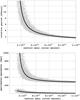 |
Fig. 1 Orbital period, pericenter, and apocenter for Leo I shown as functions of the central mass in the point mass potential, calculated according to Leo I’s Galactocentric position and velocity given in Sohn et al. (2013). The gray dots represent random values for bound (elliptic) orbits admissible within errors. |
the central mass should be much higher than 2 × 10¹² M⊙, if one agrees
that the orbital period of a relaxed bound object should be much lower than the Hubble
time. (Leo I is often included in the Jeans analysis which by definition assumes a
stationary relaxed system of tracers.) Furthermore, it would be unreasonable to expect the
apocenter of a MW’s satellite (that is, a body not affected gravitationally by the
presence of other neighboring high-mass concentrations, like M31) to be close to, or
further than halfway distance between large galaxies in the Local Group, which is
≈350 kpc. This gives at least
3 × 10¹² M⊙ for the MW
mass, as seen from Fig. 1. Also, the timing argument
(Kahn & Woltjer 1959) leads to a
comparable mass  (Sohn et al. 2013). But a timing argument is likely to
overestimate the true mass, as van der Marel &
Guhathakurta (2008) noticed for the M31-MW system, even by a factor of
2. Such high mass is also
improbable according to the argument by Wang et al.
(2012): the probability that MW’s ΛCDM halo has the observed number of subhalos with a given maximum
circular velocity, decreases steeply with increasing MW’s virial mass, effectively
vanishes for Mvir > 3 × 10¹² M⊙,
and is only 5% for
Mvir > 2 × 10¹² M⊙.
Therefore, the MW mass cannot be too high, so the timescale for Leo I must be within an
order of magnitude of the Hubble time. This contradicts the assumption that the time scale
is much lower.
(Sohn et al. 2013). But a timing argument is likely to
overestimate the true mass, as van der Marel &
Guhathakurta (2008) noticed for the M31-MW system, even by a factor of
2. Such high mass is also
improbable according to the argument by Wang et al.
(2012): the probability that MW’s ΛCDM halo has the observed number of subhalos with a given maximum
circular velocity, decreases steeply with increasing MW’s virial mass, effectively
vanishes for Mvir > 3 × 10¹² M⊙,
and is only 5% for
Mvir > 2 × 10¹² M⊙.
Therefore, the MW mass cannot be too high, so the timescale for Leo I must be within an
order of magnitude of the Hubble time. This contradicts the assumption that the time scale
is much lower.
High masses from the timing argument are also inconsistent with recent mass estimates.
The favored model in (Klypin et al. 2002) gives
1012 M⊙ for the virial mass
of the MW. Xue et al. (2008) estimate the MW mass
to 4.0 ± 0.7 × 10¹¹ M⊙ within
60 kpc from the kinematics
of a large virialized sample of BHB stars, and extrapolate this result to the MW’s dark
halo mass  . Deason et al. (2012b) suggest that the mass within
150 kpc is probably in the
range from 5.0 × 10¹¹ M⊙ to
10.0 × 10¹¹ M⊙ and that
there may be low mass between 50 and 150 kpc
(implying a high-concentration halo). The authors come to the conclusion that Leo I is
almost certainly unbound. Next, Di Cintio et al.
(2013) conclude with the MW’s mass is between 5.5−7.5 × 10¹¹ M⊙. Another
recent work (Vera-Ciro et al. 2013) finds that the
number and internal dynamics of the classical dwarf spheroidal satellites will be
consistent with the predictions of the ΛCDM model, if the MW total mass is 8.0 × 10¹¹ M⊙, again
insufficient to bind Leo I to the MW. The latter value was obtained in the past as the
upper bound for the mass at the 99% confidence level, by assuming an isotropic velocity distribution
for objects at distances of 50−140 kpc (Little &
Tremaine 1987), with the reservation that this estimate can be lower for more
radial orbits.
. Deason et al. (2012b) suggest that the mass within
150 kpc is probably in the
range from 5.0 × 10¹¹ M⊙ to
10.0 × 10¹¹ M⊙ and that
there may be low mass between 50 and 150 kpc
(implying a high-concentration halo). The authors come to the conclusion that Leo I is
almost certainly unbound. Next, Di Cintio et al.
(2013) conclude with the MW’s mass is between 5.5−7.5 × 10¹¹ M⊙. Another
recent work (Vera-Ciro et al. 2013) finds that the
number and internal dynamics of the classical dwarf spheroidal satellites will be
consistent with the predictions of the ΛCDM model, if the MW total mass is 8.0 × 10¹¹ M⊙, again
insufficient to bind Leo I to the MW. The latter value was obtained in the past as the
upper bound for the mass at the 99% confidence level, by assuming an isotropic velocity distribution
for objects at distances of 50−140 kpc (Little &
Tremaine 1987), with the reservation that this estimate can be lower for more
radial orbits.
Leo I is a kinematical outlier from the rest of velocity tracers. In this context we recall that the statistical analysis of data advises not including single measurements that evidently are well outside the range of other data. It would hardly be an acceptable situation if the MW mass was determined using a single tracer (while it is uncertain whether it is bound or not). By the mere assumption that Leo I is bound, one would have to accept a lower limit for the MW mass of at least 1.16 × 10¹², even though motions of a vast majority of remaining tracers or other arguments as in Wang et al. (2012) might point to a lower mass, insufficient to bind Leo I. As tested by Deason et al. (2011), including unbound satellites in two popular mass estimates (Bahcall & Tremaine 1981; Watkins et al. 2010) can cause large overestimates of the true mass. Leo I disproportionately affects MW mass estimates under the assumption of equilibrium kinematics (Sohn et al. 2013), e.g. by adding Leo I, the mass estimate can be increased by nearly a factor of 3 (Zaritsky et al. 1989). A simple mass estimator applied to the satellite populations (Leo I discarded) gives the minimum 4 ± 1 × 10¹¹ M⊙ for enclosed mass within 300 kpc (Watkins et al. 2010), whereas including Leo I would increase the estimate to 15.0 ± 4.0 × 10¹¹ M⊙. By using a halo model (Wilkinson & Evans 1999) with variable anisotropy parameter and integrable halo mass, one can show that both the mass and the length scale change a lot: when Leo I is included the most likely values are 17 × 1011 M⊙ and 150 kpc for the total halo mass and the length scale, whereas with Leo I excluded, the quantities shrink by a factor of 6 to 3.0 × 10¹¹ M⊙ and 25 kpc. According to us, determination of mass should be stable against inclusion/exclusion of a sufficiently small subsamples of velocity tracers. With Leo I this is by no means possible.
As it was suggested in Sohn et al. (2013), there might be a 77% chance that Leo I could be bound to the MW. However, the same authors conclude that it would not necessarily be appropriate to include Leo I in equilibrium models used to estimate the MW virial mass. The kinematics of Leo I is unlikely to be virialized on account of its expected first infall into the MW. It was concluded in Byrd et al. (1994), that the history of the local group is too complex to justify calculating the mass of the MW by assuming that all satellites of our galaxy are bound. Second, a more prosaic scenario cannot be excluded: Leo I may have passed coincidentally by us, and could have originated outside the MW (Zaritsky et al. 1989). Third, as observed in Sales et al. (2007), fast receding satellites, such as Leo I, can be present owing to a three-body ejection mechanism, which is propelling bodies into highly energetic orbits.
Given the above arguments, it seems most likely that Leo I must be a member of a higher mass concentration and cannot be bound to the MW alone. We therefore discard Leo I from further analysis.
2.2. Two samples of tracers
When the MW’s mass is expected to be lower, as suggested by the discussion in Sect. 1, some of the tracers cannot be gravitationally bound to
it and, therefore, similar to Leo I, should not be included in preparing the RVD profile.
The following criterion can be used for hypothesizing which of satellites might be
unbound. The simple calculation of Sect. 1 leads to
the mass estimator  with
μ = 4 for
β ≈ 0 (or
β ≈ ϵ/2 with a
small ϵ > 0), where the summation
is taken over a number Nr of objects with
the radial distance not lower than r. This result follows at once for an approximately
flat , when one can use
instead, but it can also be
arrived at without this reservation by applying Eq. (23) given in Watkins et al. (2010) with suitable parameters. As can be seen in Fig.
2,
with
μ = 4 for
β ≈ 0 (or
β ≈ ϵ/2 with a
small ϵ > 0), where the summation
is taken over a number Nr of objects with
the radial distance not lower than r. This result follows at once for an approximately
flat , when one can use
instead, but it can also be
arrived at without this reservation by applying Eq. (23) given in Watkins et al. (2010) with suitable parameters. As can be seen in Fig.
2,
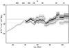 |
Fig. 2 Mean values |


the mass estimate  (μ ≈ 4) is approximately
invariable in the region from 40 kpc to 90 kpc, consistently with what one would expect for a compact
concentration of mass. (Beyond 90 kpc the statistics is too small.) This is in accord with the
value 3.5−5 × 10¹¹ M⊙ within
150 kpc, obtained in a
Keplerian halo model (Deason et al. 2012b). With
the limiting value μ = 2 for β = 1,
(μ ≈ 4) is approximately
invariable in the region from 40 kpc to 90 kpc, consistently with what one would expect for a compact
concentration of mass. (Beyond 90 kpc the statistics is too small.) This is in accord with the
value 3.5−5 × 10¹¹ M⊙ within
150 kpc, obtained in a
Keplerian halo model (Deason et al. 2012b). With
the limiting value μ = 2 for β = 1,  might be as low as 2.1−2.6 × 10¹¹ M⊙ (see,
the straight lines in Fig. 2). The two estimates
suggest that satellites with
might be as low as 2.1−2.6 × 10¹¹ M⊙ (see,
the straight lines in Fig. 2). The two estimates
suggest that satellites with  greater
than 5 × 10¹¹ M⊙ or
3 × 10¹¹ M⊙, respectively,
might not be bound to the MW and should be excluded prior to preparing the RVD profile. We
further assume these two possibilities by considering two samples of tracers SI and SII as
specified in Table 1.
greater
than 5 × 10¹¹ M⊙ or
3 × 10¹¹ M⊙, respectively,
might not be bound to the MW and should be excluded prior to preparing the RVD profile. We
further assume these two possibilities by considering two samples of tracers SI and SII as
specified in Table 1.
Radial velocity tracers with the largest  and samples SI and SII used in the text.
2.3. The radial velocity dispersion profile
As explained in Sect. 2.2, we consider two RVD profiles based on tracers from samples SI and SII (see Table 1). The PDFs are shown in Fig. 3
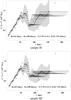 |
Fig. 3 Radial velocity dispersion (RVD) profiles |

and also compared in Fig. 4, in the background of all tracers.
The RVD curves in Fig. 3 were obtained as follows:
for any ri all of
ni tracers are taken
inside a spherical shell |r − ri| < w/2
of a fixed width w. When necessary, w is increased so that
ni is never lower than
some fixed n,
which effectively increases the bin size at large radii where the statistics are poor
because there were few tracers. Then m random subsets of size
 are chosen, and
a quartet of numbers is assigned to each of them: two mean values ⟨ r ⟩ and
are chosen, and
a quartet of numbers is assigned to each of them: two mean values ⟨ r ⟩ and
 , and
two numbers rmin and rmax, the
smallest and the largest r in each subset. This is repeated for all
ri at various
n. Then an
ordered list consisting of all the quartets is formed, sorted according to increasing
⟨ r ⟩.
Finally, a moving average is performed over quartets with ⟨ r ⟩ falling in a window
of width W,
when the window moves through the entire range of r. In effect, a curve is
obtained on the plane
, and
two numbers rmin and rmax, the
smallest and the largest r in each subset. This is repeated for all
ri at various
n. Then an
ordered list consisting of all the quartets is formed, sorted according to increasing
⟨ r ⟩.
Finally, a moving average is performed over quartets with ⟨ r ⟩ falling in a window
of width W,
when the window moves through the entire range of r. In effect, a curve is
obtained on the plane  . We assumed w = 9 kpc,
m = 89,
W = 6 kpc, and n from 15 to 22. For each r the horizontal “error
bars” represent the intervals ⟨ rmin ⟩ < r < ⟨ rmax ⟩,
while the vertical “error bars” represent the standard deviations of
times
. We assumed w = 9 kpc,
m = 89,
W = 6 kpc, and n from 15 to 22. For each r the horizontal “error
bars” represent the intervals ⟨ rmin ⟩ < r < ⟨ rmax ⟩,
while the vertical “error bars” represent the standard deviations of
times
 ,
and measure a Monte Carlo-like estimate of the uncertainty in
due to
various subsets of tracers taken in obtaining the mean values
.
,
and measure a Monte Carlo-like estimate of the uncertainty in
due to
various subsets of tracers taken in obtaining the mean values
.
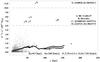 |
Fig. 4 Radial velocity tracers (gray dots/black stars) and the radial velocity dispersion
(RVD) profiles (black circles) of Fig. 3 shown
on the |

It can be seen that the RVD profiles largely depend on two tracers with the highest
 , B, and X,
while the inclusion/exclusion of the other three tracers A, C, and D, is not so decisive.
Tracer X certainly cannot be bound to the MW due to the recent low-mass estimates referred
to earlier and therefore should not be included. This consideration substantiates our
choice of the two basic RVD profiles.
, B, and X,
while the inclusion/exclusion of the other three tracers A, C, and D, is not so decisive.
Tracer X certainly cannot be bound to the MW due to the recent low-mass estimates referred
to earlier and therefore should not be included. This consideration substantiates our
choice of the two basic RVD profiles.
The RVD profiles in Fig. 3 can be interpolated to form continuous curves that can be regarded as smooth model curves, consistent with the measurements within certain uncertainty limits6. With the aid of the method introduced in Sect. 3.1.3, a number of PDFs can be found, giving rise to the respective theoretical RVD curves consistent with the smooth model curves within the same limits. When this is possible with some mass M, we say that the M, as an estimate for the MW mass, accounts for the radial motions of tracers.
3. Keplerian ensemble method
To estimate the lower bound for the MW mass, we assume that external tracers move as test bodies in the host gravitational field of a compact mass distribution. In this case, at sufficiently large radii, a contribution from the higher multipoles of the field should be small compared to the monopole part, and the motion of distant test bodies should be approximately describable in terms of Keplerian orbits. Because point mass formulae can be used as order-of-magnitude estimates of gravitating mass, the compactness assumption does not necessarily reject the possibility that an extended massive dark matter halo may be present. Also, the compactness assumption does not a priori reject the possibility that the spatially extended dark matter halo component may be absent. The latter hypothesis should be tested in accordance with Occam’s razor rule, before one decides to introduce new forms of matter, such as a ubiquitous invisible substance consisting of dark matter particles of unknown nature and, so far, eluding detection in the laboratory by producing no observable non-gravitational effects (e.g., recent null results, LUX Collaboration 2013).
3.1. The method
The motion of a test body in a spherically symmetric potential Φ(r) is flat. It occurs in
a plane through the center of symmetry. The plane is determined by two integrals of motion
that fix the unit vector normal to the plane. The additional two integrals are energy
E and the
magnitude of angular momentum J (both per unit mass). In terms of angular
velocity ω,
 , they read as
 and
and  .
In the special case of Newtonian potential
.
In the special case of Newtonian potential  , there
is an additional integral of motion indicating a fixed direction in the plane of motion.
, there
is an additional integral of motion indicating a fixed direction in the plane of motion.
The condition  for all
r > 0 with J ≠ 0 gives
for all
r > 0 with J ≠ 0 gives
 . We are only interested in
spatially bound orbits. Two turning points (where vr = 0) will be possible
for E < 0 and
. We are only interested in
spatially bound orbits. Two turning points (where vr = 0) will be possible
for E < 0 and
 . Elliptical orbits are
therefore possible only for pairs (E,J) such that
. Elliptical orbits are
therefore possible only for pairs (E,J) such that
 . Elliptical motion can be
thus uniquely determined by specifying five numbers: three Euler angles describing
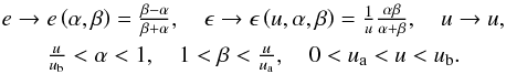
orientation of the orbit in space, and a pair of numbers (e,ϵ) defined by
. Elliptical motion can be
thus uniquely determined by specifying five numbers: three Euler angles describing
orientation of the orbit in space, and a pair of numbers (e,ϵ) defined by
 ,
0 ≤ e < 1, and
,
0 ≤ e < 1, and
 . Here, R is an arbitrary unit of
length, e the
eccentricity, and ϵ a measure of energy determining the length of the
large semi-axis, which is
. Here, R is an arbitrary unit of
length, e the
eccentricity, and ϵ a measure of energy determining the length of the
large semi-axis, which is  .
The turning points are
.
The turning points are  .
The dimensionless parameters (e,ϵ) play the central role in further
considerations.
.
The dimensionless parameters (e,ϵ) play the central role in further
considerations.
To find various expectation values for a spherically symmetric collection of confocal
ellipses (called a Keplerian ensemble), it suffices to know a PDF that describes the
number of ellipses with various e and ϵ. It will be related to the distribution function
f(r,v)
in μ-phase-space. We assume that f can be expressed through
first integrals e and ϵ. Then, f is stationary and satisfies the necessary
condition 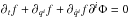 for a collisionless system. This is the wording of the Jeans theorem (Jeans 1915) in our situation. In general, the theorem
states that for a system in steady state, the PDF is a function of isolating integrals of
motion (Jeans 1915). (Under spherical symmetry two
such integrals suffice.)
for a collisionless system. This is the wording of the Jeans theorem (Jeans 1915) in our situation. In general, the theorem
states that for a system in steady state, the PDF is a function of isolating integrals of
motion (Jeans 1915). (Under spherical symmetry two
such integrals suffice.)
3.1.1. A cutoff phase-space and the resulting expectation values
The integrals of motion e and ϵ can be regarded as new, independent phase
variables. By making a transformation from ordinary spherical coordinates
r,θ,φ,vr,vθ,vφ
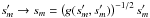
to new coordinates u,θ,φ,ϵ,e,ψ of the form r → R u,
(θ,φ) → (θ,φ),
 ,
and
,
and 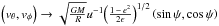 ,
the original volume element
,
the original volume element  is transformed (up
to a constant factor) to
is transformed (up
to a constant factor) to  ,
with
,
with 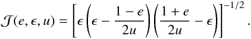 Since
we assume spherical symmetry, the angles φ, θ, and ψ can be integrated out. The remaining part of
the integration domain is determined by the function
Since
we assume spherical symmetry, the angles φ, θ, and ψ can be integrated out. The remaining part of
the integration domain is determined by the function
 .
Furthermore, in finding the expectation values as functions of r, the integration must
be taken over all ellipses that intersect a spherical thin shell of a fixed radius
r,
concentric to the center of symmetry. Given 0 < r < ∞
and 0 ≤ e < 1, we have
.
Furthermore, in finding the expectation values as functions of r, the integration must
be taken over all ellipses that intersect a spherical thin shell of a fixed radius
r,
concentric to the center of symmetry. Given 0 < r < ∞
and 0 ≤ e < 1, we have
 for such orbits. Hence, we arrive at the distribution integral
 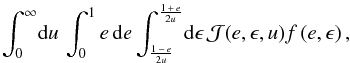 (2)which equals
 to within a
constant factor.
to within a
constant factor.
Next, for the physical reasons, we assume all orbits of the ensemble to be contained
entirely within a spherical shell R ua < r < R ub,
that is, in between two boundary spheres of radii ra = Rua
and rb = Rub.
(As a byproduct, the normalized cumulative number of objects will be automatically
integrable.) This spatial boundary imposes additional restrictions on the integration
domain in the phase-space, changing considerably the support of f(ϵ,e).
Then,  and
and  . Hence,
 and also
  . As a result, the
integration domain in the integral (2)
gets shrunk to a quadrilateral abcB, as shown in Fig. 5.
. As a result, the
integration domain in the integral (2)
gets shrunk to a quadrilateral abcB, as shown in Fig. 5.
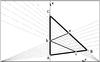 |
Fig. 5 Each point on the (e,ϵ) plane represents an elliptical orbit
with eccentricity e and energy − ϵ. The ABC
triangle with vertices A |


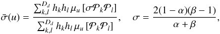
However, the integration requires splitting the u-dependent domain into
three parts. To overcome this difficulty we introduce a mapping (α,β) → (e(α,β),ϵu(α,β))
from a rectilinear region with cartesian coordinates (α,β) to a
u-dependent region abcB. This leads to the following
coordinate change in the reduced phase space (ϵ,e,u) in the above distribution integral:
 The
interpretation and the origin of this coordinate change is shown in Fig. 5. We finally get
The
interpretation and the origin of this coordinate change is shown in Fig. 5. We finally get![Mathematical equation: \begin{eqnarray} \label{eq:muIntegral} &&\skp \int f(\boldsymbol{r},\boldsymbol{v})\ud{}^3{\boldsymbol{r}}\ud{}^3{\boldsymbol{v}}\, \propto\int_{\A}^{\B}\ud{u}\,\sqrt{u}\,\mu_u[f], \qquad \mathrm{where}\\ &&\skp\mu_u[f]=\!\! \int\limits_{u/\B}^{1}\!\! \frac{\ud{\alpha}}{\sqrt{1-\alpha}} \! \int\limits_{1}^{u/\A}\!\!\!\frac{\ud{\beta}}{\sqrt{\beta-1}} \frac{\beta-\alpha}{\br{\alpha+\beta}^{5/2}}f\!\br{ \frac{\beta-\alpha}{\beta+\alpha},\frac{1}{u}\frac{\alpha\beta}{ \alpha+\beta}\!}\cdot\nonumber \end{eqnarray}](/articles/aa/full_html/2014/02/aa22617-13/aa22617-13-eq268.png) (3)Now,
given a f(e,ϵ), all expectation values
can be determined in principle. In calculating them, the following expressions are
useful:
(3)Now,
given a f(e,ϵ), all expectation values
can be determined in principle. In calculating them, the following expressions are
useful: 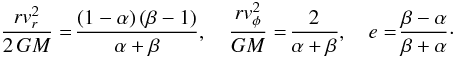 (4)For
thepurpose of further applications, the averages over concentric thin spherical shells
are important. The mean value of a function g defined on a spherical shell of radius
r, and
consequently, the average over all spherical shells can be calculated from
(4)For
thepurpose of further applications, the averages over concentric thin spherical shells
are important. The mean value of a function g defined on a spherical shell of radius
r, and
consequently, the average over all spherical shells can be calculated from ![Mathematical equation: \begin{equation} \label{expectation_value} \disp{g}_r=\frac{\mu_u[fg]}{\mu_u[f]}\quad \mathrm{and}\quad \disp{g}=\frac{\int\ud{u}\sqrt{u}\,\disp{g}_u\mu_u[f]}{\int\ud{u}\sqrt{u} \,\mu_u[f]}, \end{equation}](/articles/aa/full_html/2014/02/aa22617-13/aa22617-13-eq272.png) (5)respectively.
The expression for ⟨ g ⟩ r is quite
analogous to a conditional probability “A provided that B” for events A and B.
(5)respectively.
The expression for ⟨ g ⟩ r is quite
analogous to a conditional probability “A provided that B” for events A and B.
3.1.2. An orthogonal decomposition of the phase-space function
The problem of finding a PDF, f(e,ϵ), on a triangular domain
(Fig. 5) can be reduced to finding a series
expansion of an auxiliary function h(ξ(e,ϵ),η(e,ϵ))
in a basis of polynomials orthonormal on a simplex in the plane ξ,η (we assume that
f ≡ h2, then
f is
non-negative; the transformation functions ξ(e,ϵ),η(e,ϵ)
still need to be specified). To this end we apply the Gram-Schmidt method with a scalar
product 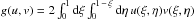 on the unit simplex
0 < ξ < 1,
0 < η < 1,
ξ + η < 1.
First, we define two families of polynomials of degree that does not exceed a given
d > 0, namely,
An,k: ηkξn−k − ξkηn−k
and Sn,k:
ηkξn−k + ξkηn−k,
with 0 ≤ n ≤ d, 0 ≤ k ≤ n. By symmetry, any
A is
orthogonal to any S. Then, we sort polynomials S, to get a sequence with
a nondecreasing degree and take their union, thereby obtaining a reduced sequence
S′. We transform S′ to another
sequence by the consecutive projections
on the unit simplex
0 < ξ < 1,
0 < η < 1,
ξ + η < 1.
First, we define two families of polynomials of degree that does not exceed a given
d > 0, namely,
An,k: ηkξn−k − ξkηn−k
and Sn,k:
ηkξn−k + ξkηn−k,
with 0 ≤ n ≤ d, 0 ≤ k ≤ n. By symmetry, any
A is
orthogonal to any S. Then, we sort polynomials S, to get a sequence with
a nondecreasing degree and take their union, thereby obtaining a reduced sequence
S′. We transform S′ to another
sequence by the consecutive projections 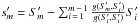 and normalize
 . We
repeat the same procedure for nonzero polynomials A to obtain a sequence
am′.
Finally, we take the union of sequences sm and
am′, and
sort with respect to the increasing degree, obtaining the required basic polynomials
. We
repeat the same procedure for nonzero polynomials A to obtain a sequence
am′.
Finally, we take the union of sequences sm and
am′, and
sort with respect to the increasing degree, obtaining the required basic polynomials
 ,
j = 0,1,...,(d + 1)(d + 2)/2.
The initial 45 polynomials
obtained this way are shown in Fig. 6.
,
j = 0,1,...,(d + 1)(d + 2)/2.
The initial 45 polynomials
obtained this way are shown in Fig. 6.
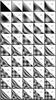 |
Fig. 6 Contour maps (with a certain automatic shading function) of 45 initial polynomials from a basis of polynomials orthonormal with respect to a standard scalar product on the unit simplex ξ + η − 1 < 0, 0 < ξ < 1, 0 < η < 1, constructed using the procedure of Sect. 3.1.2 |
Finally, we make a coordinate change  ,
,
 ,
thereby mapping the simplex to the triangular domain ABC in Fig. 5. This way, the task of finding an orthonormal basis, of
Dd = (d + 1)(d + 2)/2
polynomials
,
thereby mapping the simplex to the triangular domain ABC in Fig. 5. This way, the task of finding an orthonormal basis, of
Dd = (d + 1)(d + 2)/2
polynomials  of degree not exceeding d in e and ϵ, has been completed.
3.1.3. Finding the phase-space function and the derived quantities
The theoretical RVD can be compared with the quantity
determined based on measurements for a large enough sample of points ri. Given
d and
mass M,
this comparison enables us to find a set of optimal coefficients in the following
expansion of the phase-space function f(e,ϵ): 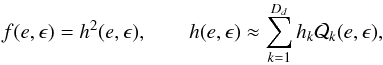 (6)byminimizing the
following mismatch function:7
(6)byminimizing the
following mismatch function:7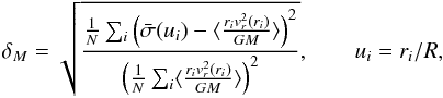 (7)N = ∑ i1 (it suffices
that N be
several times greater than Dd), where
(7)N = ∑ i1 (it suffices
that N be
several times greater than Dd), where
 (8)with
 and
and  substituted in
  s
for e and
ϵ,
respectively. The integrals
s
for e and
ϵ,
respectively. The integrals  and
and  defining functions of a single argument u leads to integrals of the
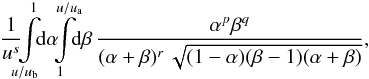 with
integers p,q,r,s. The analytical form of this integral can
be found recursively for any set of integers p,q,r.8
with
integers p,q,r,s. The analytical form of this integral can
be found recursively for any set of integers p,q,r.8
Since δM is homogenous
with degree 1 in the
variables hk, it only depends
on points on a (Dd − 1)-dimensional
unit sphere. To find the δM, one starts with
a random point on that sphere (with the help of a generator uniform on that sphere), and
then the minimization procedure is run. There can be many such minima, or a minimum can
be degenerated. Having found hk with this method,
secondary quantities other than  can be computed, using definitions like (4). They lead to expressions
  ,
,
 ,
etc., of the same general form as that of
in (8) (with quantities of the kind as
in (4) substituted for σ in
),
that is, a quotient of two quadratic forms in Dd variables
hi.
,
etc., of the same general form as that of
in (8) (with quantities of the kind as
in (4) substituted for σ in
),
that is, a quotient of two quadratic forms in Dd variables
hi.
4. Results
Using the minimization method of Sect. 3.1.3, we started by generating several best fit curves to the RVD profile of the SII sample of tracers and assumed various central masses M, ranging from90.5 × 1011 M⊙ to 50 × 1011 M⊙. This allowed us to compare the quality of best fits measured by the mismatch function δM defined in (7) and to see how it changes with the number Dd of polynomials used in (6) to approximate the PDF. The result of this comparison is presented in Fig. 7,
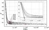 |
Fig. 7 A χ2-like test defined by δM for best-fit curves to the RVD profile of sample SII (see Fig. 3, bottom panel) shown as a function of the central mass M. The phase-space support used to obtain these results was fixed by ua = 18 kpc and ub = 300 kpc, and the fitting region was limited to r > 22 kpc. One can distinguish 5 accumulation curves that correspond to various degrees d of polynomials used to approximate the phase distribution function (here, d = 4,5,6,7,8). These curves were compared with best-fitting hyperbolas in the inset panel. Abscissae of crossing points of the corresponding asymptotes suggest the presence of a lower bound for mass in the limit of large d. The red dots represent minimum values of δM found at M = 2.4 × 10¹¹ M⊙ and, to compare with, at M = 1.0 × 10¹² M⊙ (for d = 8 points with ub = 240 kpc were also included). |
where δM is shown versus the central mass M for various d. The example best-fit curves to the RVD profile (assuming d = 8) were compared in Fig. 8.
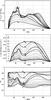 |
Fig. 8 Top: example best-fit curves to the RVD profile of sample SII for masses ranging from 0.5 × 10¹¹ M⊙ to 10 × 1011 M⊙ (A: 0.5 × 10¹¹ M⊙, B: 1.02 × 10¹¹ M⊙, C: 1.3 × 10¹¹ M⊙, D: 2.09 × 10¹¹ M⊙, E: 2.4 × 10¹¹ M⊙, F: 10.2 × 10¹¹ M⊙), assuming d = 8 and ua = 18 kpc, ub = 240 kpc (⇒0 < e < 0.83). The light gray region is the uncertainty in the RVD profile corresponding to vertical bars in Fig. 3. Middle: corresponding (symmetrized) anisotropy parameter. Bottom: mean eccentricity. |
Lower panels in Fig. 8 show the corresponding secondary quantities. As expected, they can change significantly when RVD best-fit curves are not changed at all. This illustrates our earlier theoretical expectation that M cannot be determined based on the measurements of the radial motions alone. Also, due to the flattening of the δM curves in Fig. 7 for high masses, the optimum mass, chosen to correspond to the lowest δM fit (a global minimum), would have unacceptably large uncertainty (as would the secondary quantities that are largely M-dependent). Thus, the criterion of mass must be different. Nevertheless, one can estimate a lower bound for M.
As can be seen in Fig. 7, for high enough M, δM gets reduced when d is increased and appears to tend to some small nonzero limit, and the same for all M when d is large enough. For lower M, δM decreases faster with increasing d than previously, but for d large enough the attained limit seems the same as for larger M. For even lower masses, below 2 × 10¹¹ M⊙, the mismatch function δM grows rapidly. With low enough M, therefore, it is not possible to obtain a satisfactory best fit curve. The diagram in Fig. 7 suggests that there is a sharp lower bound for M in the limit of large d. The presence of such a lower bound can be inferred from the observation that for a given δ, d can be increased so that M is reduced significantly to a value M − ΔM with the same quality criterion δM = δM−ΔM = δ fulfilled. For example, as seen in Fig. 7, a model with d = 6 and a high mass M = 10 × 1011 M⊙ (a value that would be accepted without hesitation in the dark-matter halo paradigm) passes the same χ2-like-test as another model with d = 8 and more than four times lower mass M = 2.4 × 10¹¹ M⊙. With larger d, the same level of δ would be attained even for a lower mass M. The crossing point of the asymptotes in Fig. 7 obtained based on the shown data, determines the approximate value for the expected minimal δ possible in the theoretical limit d → ∞ (the saturation value), and the corresponding minimal mass – the lower bound for M.
Overall, the minimum value for δM, at any M from the right-hand neighborhood of the lower bound for masses, appears to saturate in the limit of large d and remains invariable in a wide range of masses. (Already for d = 8 the δM is nearly saturated for larger masses, therefore – except for leading to insignificant reduction in δM – considering d > 8 introduces nothing new to our qualitative analysis.) The presence of the nonzero saturation value for δM indicates that the particular shape of the RVD curve cannot be exactly accounted for by the Keplerian ensemble model, irrespective of the assumed mass (but perfection is not what is expected from a model). The really important lesson we can learn from the model is that for all masses greater than some limit, the saturation value for δM is low and comparable. It means that the best-fit curves to the RVD profile are equally good, independent of mass. Putting this differently, the application of the χ2-like criterion defined by δM cannot distinguish between the admissible masses, since one cannot tell any difference between the corresponding best fits: the mass could be low (but bounded from below), as well as arbitrarily high. The RVD profile alone is thus insufficient for sharply determining the real mass, although it suffices for estimating the lower bound for admissible masses. Some other observables or conditions imposed on them must be taken into account to constrain the MW mass. However, these constraints should be imposed with due care in order not to overestimate the MW mass unnecessarily.
We have seen that M cannot be determined with the help of the best-fit
criterion. Instead, one can assume a certain M and see if the resulting secondary quantities are
plausible. As an example, we take the reference mass M = 2.4 × 10¹¹ M⊙,
which was inferred in the past from the Galaxy rotation inside 20 kpc (Merrifield 1992). This mass value also overlaps with the median value
 , found in point
potential with isotropic velocities (Little &
Tremaine 1987) for a sample of ten satellites in the Galactic halo at distances
50−140 kpc (not
including Leo I), which was deemed the most reliable one among other samples considered by
these authors. Assuming the reference mass, we performed a large number of minimizations,
starting from various initial points chosen randomly on the (Dd − 1)-dimensional unit
sphere of expansion coefficients hk. Normally, one would
expect convergence to a unique minimum (or several isolated minima), regradless of the
starting point. Instead, we found a submanifold of minima on that sphere, giving rise to a
number of best-fit curves through the measured RVD, as shown in Fig. 9 (upper panels). Although the sets of expansion parameters (thus also the
corresponding PDFs) are different, the corresponding best-fit curves to the same profile of
the radial velocity dispersion are almost indistinguishable.
, found in point
potential with isotropic velocities (Little &
Tremaine 1987) for a sample of ten satellites in the Galactic halo at distances
50−140 kpc (not
including Leo I), which was deemed the most reliable one among other samples considered by
these authors. Assuming the reference mass, we performed a large number of minimizations,
starting from various initial points chosen randomly on the (Dd − 1)-dimensional unit
sphere of expansion coefficients hk. Normally, one would
expect convergence to a unique minimum (or several isolated minima), regradless of the
starting point. Instead, we found a submanifold of minima on that sphere, giving rise to a
number of best-fit curves through the measured RVD, as shown in Fig. 9 (upper panels). Although the sets of expansion parameters (thus also the
corresponding PDFs) are different, the corresponding best-fit curves to the same profile of
the radial velocity dispersion are almost indistinguishable.
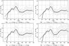 |
Fig. 9 Thick lines: mean of best-fit curves to radial velocity profiles (RVD); dotted lines: measured RVD profiles of samples SII and SI, obtained with the help of the minimization procedure of Sect. 3.1.3 assuming d = 8 and M = 2.4 × 10¹¹ M⊙. (The curve’s width equals twice the standard deviation from the mean.) The light gray region is the uncertainty in the RVD profile corresponding to vertical bars in Fig. 3. Here, rs is the left bound for the fitting region, while ra and rb determine the triangular support ABC in Fig. 5. |
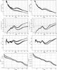 |
Fig. 10 Top: mean value and spread of secondary quantities for models that
are within the uncertainty range in Fig. 9:
dispersion of transversal velocity |


This degeneracy was to be expected, based on the indeterminacy of the Jeans problem discussed in the introduction. Choosing various sets of hk is tantamount to considering various solutions of Jeans equation with the same mass model. Hence, while a best-fit curve is not changed when hk are varied inside that manifold, the corresponding secondary quantities may change. This is indeed the case, which can be seen in Fig. 10 (lower panels), where the most important secondary quantities corresponding to the best-fit curves are shown. Interestingly, this change in the secondary quantities is not dramatic, since the spread of secondary quantities about their mean values is quite moderate.
Another source of degeneracy in the space of parameters { hk } comes from the uncertainty in the RVD profile. When one makes some variation of the RVD within the uncertainty bars and then performs the minimization procedure, the resulting expansion parameters { hk } will remain in some small neighborhood of the initial minimum. Therefore, there are many distribution functions f(e,ϵ) consistent with the RVD observations within a given uncertainty limit (error bars). This shows that the observational constraints other than RVD are needed to narrow down the range of admissible distribution functions.
5. Summary and concluding remarks
We conjectured that galactic masses may be overestimated by restricting the variety of solutions available in the framework of unconstrained Jeans modeling. These restrictions arise through imposing some subsidiary conditions when finding solutions to Jeans equations. The conditions concern mainly the velocity anisotropy profile, the form of which is often assumed and, most frequently, set constant. In this context, a simple consideration of Sect. 1 led us to the question of finding a lower bound for the MW mass, which would be consistent with the observed radial motions of distant tracers. That question motivated the main part of our work (Sects. 3 and 4), which was aimed at testing our expectation that the estimated mass value could be reduced with more general solutions to Jeans equations. We illustrated this possibility on the example of point mass field, which is tractable in an analytical way and should approximate to some extent the galactic gravitational field at large radii. In future work, we expect an analogous reduction in mass estimates to occur for more realistic mass profiles.
The principal quantity derivable from a phase-space distribution function (PDF) and used to infer the total mass is the theoretical radial velocity dispersion (RVD) profile that can be compared with the observed one. In obtaining a RVD profile from observations, one should not include gravitationally unbound bodies. (In obtaining stationary Jeans equations, one assumes that boundary surface integrals vanish at infinity, that is, no outflow of matter is possible.) In this context, we gave arguments in Sect. 2.2 that a fast receding spheroidal dwarf galaxy Leo I (and a few other objects) may not be bound to the MW and, for this reason, should be rejected at the stage of preparing the observed RVD (with Leo I included, i.e., bound to the MW, the whole analysis based on Jeans modeling to infer total mass would become quite meaningless, even when finally predicting a low mass, since within 250 kpc the total mass can be easily estimated from the escape argument for Leo I to be at least of ≈1.2 × 10¹² M⊙, or from the timing argument for Leo I to be 2−3 × 10¹² M⊙).
In Sect. 2.3, using tracers collected from recent literature, we performed a simple Monte-Carlo simulation to obtain a smooth model curve representing the observed MW’s RVD profile within estimated uncertainties. We prepared two such model curves (see Fig. 3), corresponding to two samples of tracers, SI and SII (see Table 1). The first sample was obtained assuming that both Leo I and a fast and distant BHB star J160826.42+065542.3 are not bound to the MW. The second sample discards an additional four tracers (including Hercules). We stress, however, that on comparing the two RVD profiles (see, Fig. 4), one must arrive at the conclusion that the inclusion or exclusion of the four tracers does not influence the PDF profile significantly, and that only the BHB star and Hercules make a difference. Thus the exclusion effectively concerned two tracers that were decisive for the shape of RVD profile. Either way, the present paper aimed to show the possibility of reducing mass estimates for a given sample of tracers. We consider this possibility more important than the very different problem of which of the three objects (mentioned above) are gravitationally bound to the MW.
Applying the point-mass approximation, we hypothesized that most of the matter in the MW may be more compactly distributed in space than thought so far, such that the tracers beyond a boundary region 20−25 kpc could be regarded as test bodies moving in a nearly point source field. From the standpoint of the distant tracers, the central mass of the field can be effectively used as a substitute for true galaxy mass. Accordingly, we appropriately cut off the support of the PDF to exclude orbits penetrating the internal region, where the enclosed galactic mass is not yet saturated to the value of the substitute central mass, and where the point-mass approximation may not yet apply. In the boundary region’s vicinity, where the central mass may be higher than the true mass function, this exclusion enables the theoretical RVD profile to be reduced effectively, so that it can overlap with the RVD value observed in this region. The mechanism of this reduction is simple. Elliptical orbits can osculate the boundary region only with their apocentric parts. As a result, the radial component of motion is small (with large tangential motion). For more circular orbits, which mimic the circular motion in the galactic disk, the radial motion is also minimal. However, the question of the motion of closer tracers is not that important for total mass estimations. These tracers carry the information mainly about the peculiarities in the internal distribution of mass, rather than on the total mass value. In the internal region (which we excluded by cutting off the PDFs support) or close to the boundary region, one could rightly expect some corrections to occur to the secondary quantities inferred in the point-mass approximation. But more realistic mass profiles in the interior cannot change the total mass estimate, which is mainly based on the radial motions of distant tracers. For a better determination of the total mass, it is far more important to have a significantly larger sample of external velocity tracers and (hopefully in the nearest future) complete measurements of the transversal motion.
Estimating galactic masses in the point-mass approximation showed up fruitful and widely used in the literature. Our approach, however, is essentially different and allows for unrestricted, mostly general solutions in the point mass field. Instead of solving Jeans equations involving the secondary quantities related to some unknown PDF, we looked for the PDF directly with the help of the Keplerian ensemble method we developed in Sect. 3. Our PDF satisfies the collision-less Boltzmann equation and is positive definite by construction. This way, we avoided the problem characteristic of Jeans modeling that solutions of Jeans equations do not necessarily lead to physical, non-negative PDFs. We decided to work in this approximation for two reasons. First, the spatial orbits are explicitly known, and some exact formulas in the phase-space are obtained more easily and more straightforwardly than for more complicated mass profiles. Secondly, the approximation is natural for testing our hypothesis of compact mass distribution in the MW.
The Keplerian ensemble method introduced in Sect. 3 shows how to deal with a continuous collection of confocal elliptical orbits under spherical symmetry and how to use it in practice. We allowed for a general PDF being a function of two constants of motion and with appropriately cutoff support. The secondary quantities such as the theoretical RVD, are obtained directly from the PDF and can be quite general functions of the radial variable. In this method, a particular PDF is found by minimizing the discrepancy between theoretical and measured RVD profiles. We applied our method to estimating the lower bound for the MW mass. To this, we used sample SII. Based on the observation in caption to Fig. 2 in Sect. 2.2, we can expect that a similar study for sample SI would lead to masses that are higher by a factor of 1.16 ≈ 1.2.
Both on the theoretical grounds in Sect. 1 and by interpreting our numerical results of Sect. 4, we came to the conclusion that there is no natural upper limit for the mass estimate: with the same RVD profile, the MW mass could equally well be as high as 1012 M⊙ or even higher. The absence of such a limit shows that Jeans modeling as a means of deducing the total gravitating mass from the radial motions alone is highly underdetermined. (The known mass-anisotropy degeneracy is a particular example.) As a consequence, the mass is highly model-dependent and not entirely constrained by measurements of the radial motions. The criterion for mass must be different. Based on these observations in the point mass field, one should expect an even higher degree of arbitrariness to occur in more general situations of spatially extended mass distributions. The indeterminacy shown has also an epistemological significance since the total mass, being a quantity asymptotic by its nature, should be determinable from motions of external tracers, whereas the only measurements currently available at large radii (the radial motions) are scant so cannot be conclusive.
By applying the Keplerian ensemble method, we found in Sect. 4 using sample SII that a MW mass as small as 2.4 × 10¹¹ M⊙ can still be consistent with the radial motions of tracers. We chose this example value because it is greater than the approximate lower bound of about 2.0 × 10¹¹ determined for sample SII in Fig. 7, and it agrees with the mass value obtained based on the MW rotation curve inside 20 kpc (Merrifield 1992). Interestingly enough, the same value coincides with the total MW mass obtained by Little & Tremaine (1987) in the point mass field for a sample of distant satellites. Thus, by choosing the MW mass of 2.4 × 10¹¹ M⊙, we would have both consistency with the MW’s rotation curve out to 20 kpc and excellent approximation of the galactic potential by a point mass field in the region outside 20 kpc, where we applied our Keplerian ensemble method to infer the MW mass from the radial motion of tracers. We also presented our prediction for the several secondary quantities implied by the PDF found, corresponding to the RVD at M = 2.4 × 10¹¹ M⊙. These observables could be tested when more accurate data are available at larger radii. In particular, good measurements of the tracer density profiles would provide an additional relation to be satisfied by the expansion parameters of the PDF in (6). This would in turn, be helpful in constraining the allowed bound for the MW mass in the point-mass approximation.
The possible low value of the lower bound for the MW mass is consistent with measurements in the MW interior. Dark matter is insignificant out to 5 kpc (Bissantz & Gerhard 2002). Moreover, the dynamical mass implied by the rotation of the MW inside solar radius is compatible with the mass in compact objects ascertained through microlensing measurements (Sikora et al. 2012). But there is also a recent controversy about whether the mass of MW’s interior could be that low. Depending on model assumptions, the same data on local motions of a class of tracers lead to estimates of non-baryonic dark matter in the solar vicinity differing by a large factor: see Moni Bidin et al. (2012) and the critique in Bovy & Tremaine (2012). To verify whether the total mass could indeed be that low requires further studies. As for now, one can state with certainty only the main conclusion of this paper that in the framework of Newtonian mechanics in the point mass approximation, one can find distribution functions in the phase-space that account for the radial motions of Galaxy satellites, with much lower mass than thought so far. To see the extent to which this reduction could be general, it is necessary to consider more complicated potentials in the future than the point mass that could be analyzed in a similar manner, assuming most general phase-space without a priori constraints, as this would provide better estimates for the MW mass. (As we noted, by imposing some constraints on the form of solutions to Jeans equation, one can increase the mass estimate.) We expect that a reduction in the Galaxy mass estimate similar to the one presented here for the point mass should also be possible for models assuming an extended non-baryonic dark halo.
With regard to the model of the phase-space developed here, the next step is to use base
functions on the standardized simplex of the form  ,
with
,
with  being polynomials in ξ and η, and w = ξη(1 − ξ − η)
as the weight in the scalar product. This would ensure that the phase-space distribution
function by construction vanishes smoothly on the boundary of the integration domain in the
μu integral in Eq. (3), reducing the number of spurious circular
orbits at outermost radii. It is also desirable to find best parameters ua and
ub, which are crucial for defining the
phase-space. Both these tasks are computationally more demanding, but they would improve the
results. In addition, to gain more control over secondary quantities in the minimization
procedure, one can try to impose some constraints on these quantities, provided appropriate
measurements are available.
being polynomials in ξ and η, and w = ξη(1 − ξ − η)
as the weight in the scalar product. This would ensure that the phase-space distribution
function by construction vanishes smoothly on the boundary of the integration domain in the
μu integral in Eq. (3), reducing the number of spurious circular
orbits at outermost radii. It is also desirable to find best parameters ua and
ub, which are crucial for defining the
phase-space. Both these tasks are computationally more demanding, but they would improve the
results. In addition, to gain more control over secondary quantities in the minimization
procedure, one can try to impose some constraints on these quantities, provided appropriate
measurements are available.
∂tf ≡ 0 (steady-state); dtf ≡ 0 (equilibrium) for a PDF f.
For example, the gravitational energy of a virialized self-gravitating dust is equal to minus twice the total kinetic energy. On dimensional grounds, the binding energy is a product of the total mass squared and the inverse of some characteristic size determined by the spatial distribution of dust. The total mass of a virialized system is thus a functional on the phase-space.
A good example of determining lower bounds with constraints is provided by the minimum-maximum method of finding consecutive eigenvalues and eigenvectors of a quadratic form in a finite number of dimensions or, in an infinitely dimensional function space, of a self-adjoint differential equation (Courant & Hilbert 1953).
It is not inconceivable that we can make in the nearest future more precise measurements of parameters β and ε at the outermost radii, in which case solutions of the Jeans equation would be more robust.
Here, “Keplerian” means  with γ = 1.
If need be, one can choose a subset of points on these curves with the respective “error bars” akin to the RVD data consisting of few points as usually given in the literature, such that the difference between the abscissas of the neighboring points are determined by the extension of the respective horizontal bars (e.g., a half of the mean of the extension). There are many such subsets, depending on the position of the initial point; however, all these subsets will be consistent with measurements within “errors”.
To measure the accuracy of a fit Y(x) to data points
(xi,yi),
we use a dimensionless number δ such that  , where
 . The definition of
δM agrees with that of
δ.
. The definition of
δM agrees with that of
δ.
We have not found any general formula for such an integral; however, having written a code using a computer algebra system, we were able to find the integrals in analytic form by recursions for any p,q,r. The alternative way – a numerical integration – would be inefficient in the minimization procedure; we observed that either the errors accumulated in an uncontrolled fashion, resulting in a high noise level in δM, or the computation was too time-consuming when the precision was increased to keep the errors within acceptable bounds.
Most of the values in this range of masses are physically implausible and were only used for illustration.
Acknowledgments
We would like to thank the anonymous referee for a careful reading of our manuscript and for many detailed and constructive suggestions that improved the presentation of this paper. We thank James Dwyer for interesting and stimulating discussions.
References
- An, J. H., & Evans, N. W. 2009, ApJ, 701, 1500 [NASA ADS] [CrossRef] [Google Scholar]
- Bahcall, J. N., & Tremaine, S. 1981, ApJ, 244, 805 [NASA ADS] [CrossRef] [Google Scholar]
- Beers, T. C., Preston, G. W., & Shectman, S. A. 1992, AJ, 103, 1987 [NASA ADS] [CrossRef] [Google Scholar]
- Belokurov, V., Walker, M. G., Evans, N. W., et al. 2008, ApJ, 686, L83 [NASA ADS] [CrossRef] [Google Scholar]
- Belokurov, V., Walker, M. G., Evans, N. W., et al. 2009, MNRAS, 397, 1748 [NASA ADS] [CrossRef] [Google Scholar]
- Bissantz, N., & Gerhard, O. 2002, MNRAS, 330, 591 [NASA ADS] [CrossRef] [Google Scholar]
- Bovy, J., & Tremaine, S. 2012, ApJ, 756, 89 [Google Scholar]
- Bovy, J., Hogg, D. W., & Rix, H.-W. 2009, ApJ, 704, 1704 [NASA ADS] [CrossRef] [Google Scholar]
- Bovy, J., Murray, I., & Hogg, D. W. 2010, ApJ, 711, 1157 [Google Scholar]
- Brown, W. R., Geller, M. J., Kenyon, S. J., & Diaferio, A. 2010, AJ, 139, 59 [NASA ADS] [CrossRef] [Google Scholar]
- Byrd, G., Valtonen, M., McCall, M., & Innanen, K. 1994, AJ, 107, 2055 [NASA ADS] [CrossRef] [Google Scholar]
- Carney, B. W. 1984, PASP, 96, 841 [NASA ADS] [CrossRef] [Google Scholar]
- Clewley, L., Warren, S. J., Hewett, P. C., Norris, J. E., & Evans, N. W. 2004, MNRAS, 352, 285 [NASA ADS] [CrossRef] [Google Scholar]
- Courant, R., & Hilbert, D. 1953, Methods of mathematical physics, Vols. 1, 2 (New york: Interscience Publication) [Google Scholar]
- Deason, A. J., McCarthy, I. G., Font, A. S., et al. 2011, MNRAS, 415, 2607 [NASA ADS] [CrossRef] [Google Scholar]
- Deason, A. J., Belokurov, V., Evans, N. W., & An, J. 2012a, MNRAS, 424, L44 [NASA ADS] [CrossRef] [Google Scholar]
- Deason, A. J., Belokurov, V., Evans, N. W., et al. 2012b, MNRAS, 425, 2840 [NASA ADS] [CrossRef] [Google Scholar]
- Dehnen, W., & Binney, J. 1998, MNRAS, 294, 429 [NASA ADS] [CrossRef] [Google Scholar]
- Di Cintio, A., Knebe, A., Libeskind, N. I., et al. 2013, MNRAS, 431, 1220 [NASA ADS] [CrossRef] [Google Scholar]
- Dohm-Palmer, R. C., Helmi, A., Morrison, H., et al. 2001, ApJ, 555, L37 [NASA ADS] [CrossRef] [Google Scholar]
- Francis, C., & Anderson, E. 2009, New A, 14, 615 [NASA ADS] [CrossRef] [Google Scholar]
- Geha, M., Willman, B., Simon, J. D., et al. 2009, ApJ, 692, 1464 [NASA ADS] [CrossRef] [Google Scholar]
- Harris, W. E. 1996, AJ, 112, 1487 [NASA ADS] [CrossRef] [Google Scholar]
- Jeans, J. H. 1915, MNRAS, 76, 70 [NASA ADS] [CrossRef] [Google Scholar]
- Kahn, F. D., & Woltjer, L. 1959, ApJ, 130, 705 [NASA ADS] [CrossRef] [Google Scholar]
- Klypin, A., Zhao, H., & Somerville, R. S. 2002, ApJ, 573, 597 [Google Scholar]
- Koch, A., Wilkinson, M. I., Kleyna, J. T., et al. 2009, ApJ, 690, 453 [NASA ADS] [CrossRef] [Google Scholar]
- Koposov, S. E., Rix, H.-W., & Hogg, D. W. 2010, ApJ, 712, 260 [NASA ADS] [CrossRef] [Google Scholar]
- Little, B., & Tremaine, S. 1987, ApJ, 320, 493 [NASA ADS] [CrossRef] [Google Scholar]
- LUX Collaboration 2013, Phys. Rev. Lett., submitted [arXiv:1310.8214] [Google Scholar]
- Magorrian, J. 2014, MNRAS, 437, 2230 [NASA ADS] [CrossRef] [Google Scholar]
- Martin, N. F., Ibata, R. A., Chapman, S. C., Irwin, M., & Lewis, G. F. 2007, MNRAS, 380, 281 [NASA ADS] [CrossRef] [Google Scholar]
- Mateo, M. L. 1998, ARA&A, 36, 435 [NASA ADS] [CrossRef] [Google Scholar]
- Merrifield, M. R. 1992, AJ, 103, 1552 [NASA ADS] [CrossRef] [Google Scholar]
- Moni Bidin, C., Carraro, G., Méndez, R. A., & Smith, R. 2012, ApJ, 751, 30 [NASA ADS] [CrossRef] [Google Scholar]
- Morrison, H. L., Mateo, M., Olszewski, E. W., et al. 2000, AJ, 119, 2254 [NASA ADS] [CrossRef] [Google Scholar]
- Perryman, M. A. C., de Boer, K. S., Gilmore, G., et al. 2001, A&A, 369, 339 [NASA ADS] [CrossRef] [EDP Sciences] [Google Scholar]
- Sakamoto, T., Chiba, M., & Beers, T. C. 2003, A&A, 397, 899 [NASA ADS] [CrossRef] [EDP Sciences] [Google Scholar]
- Sales, L. V., Navarro, J. F., Abadi, M. G., & Steinmetz, M. 2007, MNRAS, 379, 1475 [NASA ADS] [CrossRef] [Google Scholar]
- Schönrich, R., Binney, J., & Dehnen, W. 2010, MNRAS, 403, 1829 [NASA ADS] [CrossRef] [Google Scholar]
- Sikora, S., Bratek, Ł., Jałocha, J., & Kutschera, M. 2012, A&A, 546, A126 [NASA ADS] [CrossRef] [EDP Sciences] [Google Scholar]
- Simon, J. D., & Geha, M. 2007, ApJ, 670, 313 [NASA ADS] [CrossRef] [Google Scholar]
- Sohn, S. T., Besla, G., van der Marel, R. P., et al. 2013, ApJ, 768, 139 [NASA ADS] [CrossRef] [Google Scholar]
- Starkenburg, E., Helmi, A., Morrison, H. L., et al. 2009, ApJ, 698, 567 [NASA ADS] [CrossRef] [Google Scholar]
- van der Marel, R. P., & Guhathakurta, P. 2008, ApJ, 678, 187 [NASA ADS] [CrossRef] [Google Scholar]
- Vera-Ciro, C. A., Helmi, A., Starkenburg, E., & Breddels, M. A. 2013, MNRAS, 428, 1696 [NASA ADS] [CrossRef] [Google Scholar]
- Wang, J., Frenk, C. S., Navarro, J. F., Gao, L., & Sawala, T. 2012, MNRAS, 424, 2715 [NASA ADS] [CrossRef] [Google Scholar]
- Watkins, L. L., Evans, N. W., & An, J. H. 2010, MNRAS, 406, 264 [NASA ADS] [CrossRef] [Google Scholar]
- Wilhelm, R., Beers, T. C., Sommer-Larsen, J., et al. 1999, AJ, 117, 2329 [NASA ADS] [CrossRef] [Google Scholar]
- Wilkinson, M. I., & Evans, N. W. 1999, MNRAS, 310, 645 [NASA ADS] [CrossRef] [Google Scholar]
- Xue, X. X., Rix, H. W., Zhao, G., et al. 2008, ApJ, 684, 1143 [NASA ADS] [CrossRef] [Google Scholar]
- Zaritsky, D., Olszewski, E. W., Schommer, R. A., Peterson, R. C., & Aaronson, M. 1989, ApJ, 345, 759 [NASA ADS] [CrossRef] [Google Scholar]
All Tables
Radial velocity tracers with the largest
and samples SI and SII used in the text.
All Figures
|
Fig. 1 Orbital period, pericenter, and apocenter for Leo I shown as functions of the central mass in the point mass potential, calculated according to Leo I’s Galactocentric position and velocity given in Sohn et al. (2013). The gray dots represent random values for bound (elliptic) orbits admissible within errors. |
| In the text | |
|
Fig. 2 Mean values |
| In the text | |
|
Fig. 3 Radial velocity dispersion (RVD) profiles |
| In the text | |
|
Fig. 4 Radial velocity tracers (gray dots/black stars) and the radial velocity dispersion
(RVD) profiles (black circles) of Fig. 3 shown
on the |
| In the text | |
|
Fig. 5 Each point on the (e,ϵ) plane represents an elliptical orbit
with eccentricity e and energy − ϵ. The ABC
triangle with vertices A |
| In the text | |
|
Fig. 6 Contour maps (with a certain automatic shading function) of 45 initial polynomials from a basis of polynomials orthonormal with respect to a standard scalar product on the unit simplex ξ + η − 1 < 0, 0 < ξ < 1, 0 < η < 1, constructed using the procedure of Sect. 3.1.2 |
| In the text | |
|
Fig. 7 A χ2-like test defined by δM for best-fit curves to the RVD profile of sample SII (see Fig. 3, bottom panel) shown as a function of the central mass M. The phase-space support used to obtain these results was fixed by ua = 18 kpc and ub = 300 kpc, and the fitting region was limited to r > 22 kpc. One can distinguish 5 accumulation curves that correspond to various degrees d of polynomials used to approximate the phase distribution function (here, d = 4,5,6,7,8). These curves were compared with best-fitting hyperbolas in the inset panel. Abscissae of crossing points of the corresponding asymptotes suggest the presence of a lower bound for mass in the limit of large d. The red dots represent minimum values of δM found at M = 2.4 × 10¹¹ M⊙ and, to compare with, at M = 1.0 × 10¹² M⊙ (for d = 8 points with ub = 240 kpc were also included). |
| In the text | |
|
Fig. 8 Top: example best-fit curves to the RVD profile of sample SII for masses ranging from 0.5 × 10¹¹ M⊙ to 10 × 1011 M⊙ (A: 0.5 × 10¹¹ M⊙, B: 1.02 × 10¹¹ M⊙, C: 1.3 × 10¹¹ M⊙, D: 2.09 × 10¹¹ M⊙, E: 2.4 × 10¹¹ M⊙, F: 10.2 × 10¹¹ M⊙), assuming d = 8 and ua = 18 kpc, ub = 240 kpc (⇒0 < e < 0.83). The light gray region is the uncertainty in the RVD profile corresponding to vertical bars in Fig. 3. Middle: corresponding (symmetrized) anisotropy parameter. Bottom: mean eccentricity. |
| In the text | |
|
Fig. 9 Thick lines: mean of best-fit curves to radial velocity profiles (RVD); dotted lines: measured RVD profiles of samples SII and SI, obtained with the help of the minimization procedure of Sect. 3.1.3 assuming d = 8 and M = 2.4 × 10¹¹ M⊙. (The curve’s width equals twice the standard deviation from the mean.) The light gray region is the uncertainty in the RVD profile corresponding to vertical bars in Fig. 3. Here, rs is the left bound for the fitting region, while ra and rb determine the triangular support ABC in Fig. 5. |
| In the text | |
|
Fig. 10 Top: mean value and spread of secondary quantities for models that
are within the uncertainty range in Fig. 9:
dispersion of transversal velocity |
| In the text | |
Current usage metrics show cumulative count of Article Views (full-text article views including HTML views, PDF and ePub downloads, according to the available data) and Abstracts Views on Vision4Press platform.
Data correspond to usage on the plateform after 2015. The current usage metrics is available 48-96 hours after online publication and is updated daily on week days.
Initial download of the metrics may take a while.