| Issue |
A&A
Volume 562, February 2014
|
|
|---|---|---|
| Article Number | A58 | |
| Number of page(s) | 12 | |
| Section | The Sun | |
| DOI | https://doi.org/10.1051/0004-6361/201322462 | |
| Published online | 05 February 2014 | |
Preferential acceleration of heavy ions in the reconnection outflow region
Drift and surfatron ion acceleration
1
LPC2E/CNRS University of Orléans, UMR7328,
45071
Orléans,
France
e-mail:
ante0226@gmail.com
2
Space Research Institute, RAS, 117997
Moscow,
Russia
3
Department of Physics, University della Calabria,
87036
Arcavacata di Rende,
Italy
e-mail:
zimbardo@fis.unical.it
4 Johns Hopkins University Applied Physics Laboratory, USA
5
Institute of Space and Astronautical Science, Japan Aerospace Exploration Agency
(JAXA),
252-5210
Sagamihara,
Japan
Received:
8
August
2013
Accepted:
10
December
2013
Context. Many observations show that heating in the solar corona should be more effective for heavy ions than for protons. Moreover, the efficiency of particle heating also seems to be larger for a larger particle electric charge. The transient magnetic reconnection is one of the most natural mechanisms of charged particle acceleration in the solar corona. However, the role of this process in preferential acceleration of heavy ions has still yet to be investigated.
Aims. In this paper, we consider charged particle acceleration in the reconnection outflow region. We investigate the dependence of efficiency of various mechanisms of particle acceleration on particle charge and mass.
Methods. We take into account recent in situ spacecraft observations of the nonlinear magnetic waves that have originated in the magnetic reconnection. We use analytical estimates and test-particle trajectories to study resonant and nonresonant particle acceleration by these nonlinear waves.
Results. We show that resonant acceleration of heavy ions by nonlinear magnetic waves in the reconnection outflow region is more effective for heavy ions and/or for ions with a larger electric charge. Nonresonant acceleration can be considered as a combination of particle reflections from the front of the nonlinear waves. Energy gain for a single reflection is proportional to the particle mass, while the maximum possible gain of energy corresponds to the classical betatron heating.
Conclusions. Small-scale transient magnetic reconnections produce nonlinear magnetic waves propagating away from the reconnection region. These waves can effectively accelerate heavy ions in the solar corona via resonant and nonresonnat regimes of interactions. This mechanism of acceleration is more effective for ions with a larger mass and/or with a larger electric charge.
Key words: magnetic reconnection / acceleration of particles / Sun: corona
© ESO, 2014
1. Introduction
Some of the most puzzling observations by the SoHO spacecraft concern that heavy ions like O5+ and Mg9+ in the solar corona are heated more than protons and that the temperature of different species are more than their proportion to mass (Kohl et al. 1997, 1998; Cranmer et al. 1999; Esser et al. 1999). Also in the solar wind, alpha particles are faster and hotter than protons (e.g. Marsch & Tu 2001; Kasper et al. 2008). In addition, the heavy ion kinetic temperatures in the corona are strongly anisotropic with T⊥/T∥ ≃ 10–100, while moderate anisotropy is observed for protons, T⊥/T∥ ≃ 2–3 (Kohl et al. 1998; Esser et al. 1999), where T⊥ (T∥) represents the perpendicular (parallel) kinetic temperature.
It is worth pointing out that understanding the origin of such anisotropic and more heating of heavy ions is crucial for unravelling the mechanisms of energy conversion and heating of the solar corona. Ion cyclotron heating has been considered as a possible explanation (e.g., Marsch et al. 1982; Hollweg & Isenberg 2002), but many details are not clear. Another possibility is that the more effective heating of heavy ions is due to shock waves in the corona (Lee & Wu 2000; Zimbardo 2010, 2011). Indeed, those models show that quasi-perpendicular shocks are able to heat heavy ions more than protons, and preferential heating of heavy ions is actually observed in the solar wind on occasion of interplanetary shock crossings (Zastenker & Borodkova 1984; Berdichevsky et al. 1997). Shock waves are observed in the solar corona by UV data analysis (Mancuso et al. 2002; Bemporad & Mancuso 2010) and are also detected by type II radio bursts (Nelson & Melrose 1985), which are frequently associated with the emergence of coronal mass ejections and to flares (e.g., Tsuneta & Naito 1998; Aurass & Mann 2004). However, it is not clear whether enough shocks exist to explain the heavy ion temperatures, which are indeed present in the corona.
Here, we explore another possibility, which is the preferential heating of heavy ions at the front of coronal hole reconnection outflow jets. The classical model of a solar flare and coronal mass ejection predicts that magnetic reconnection plays an important role in these processes (e.g., Priest & Forbes 2000, and references therein). The reconnection can occur at some distance above coronal loops where the thin current sheet should be formed (Syrovatskiǐ 1971; Parker 1994). There are many indirect observations showing that this current sheet indeed exists (e.g. Ciaravella & Raymond 2008; Liu et al. 2010) and its reconnection results in release of the magnetic energy (e.g., Tsuneta 1996; Lin 2002; Aurass et al. 2009). The envisaged complimentary physical scenario for coronal holes would be that photospheric convection leads to the emergence of small magnetic bipoles, which undergo magnetic reconnection with the large scale unipolar magnetic field of coronal holes.
According to simplified 2D models (see review Priest & Forbes 2000, and references therein), the current sheet with the reconnected magnetic field lines includes inflow and outflow regions. Due to significant stretching of field lines, the relation between velocities of plasma flows in these regions should be around ~10–100, where the plasma inflow velocity is much smaller than the plasma outflow velocity (see observations by Takasao et al. 2012). Indeed, both UV and X-ray observations by STEREO, Hinode, Yohkoh, and other spacecraft show that fast jets are very common in the polar coronal holes (Shimojo et al. 1996; Cirtain et al. 2007; Patsourakos et al. 2008; Nisticò et al. 2009, 2010). Moreover, observations by Hinode and STEREO reveal the presence of fast flows and Doppler broadened lines in the low corona (Kamio et al. 2009). Such fast plasma jets can be responsible for formation of shock waves (or shock-like structures) in the outflow region (e.g. Lin et al. 2009; Guidoni & Longcope 2010). Indeed, shock waves are often considered as an important ingredient of the scenario of the magnetic reconnection in the solar corona (see reviews by Aschwanden 2002; Webb & Howard 2012). However, even if the velocity of plasma jets is not high enough to create shock-waves, the transient magnetic reconnection should produce slow shock-like structures (compressional wave front) propagating away from the X-line region. These structures are characterized by an increased magnetic field magnitude (e.g. Heyn & Semenov 1996; Longcope & Priest 2007).
Ion acceleration in the course of the magnetic reconnection is considered now as one of the most effective mechanisms in hot, weakly magnetized plasma. There are several numerical and analytical investigations of ion heating in the vicinity of the X-line and in the outflow region (e.g., Zelenyi et al. 1990; Lottermoser et al. 1998; Litvinenko 2003; Anastasiadis et al. 2008; Zharkova & Agapitov 2009). The main problem of such models corresponds to the transient nature of the magnetic reconnection, where a X-line type magnetic field configuration with strong electric fields exists only at a limited time interval. Moreover, the domain in the close vicinity of the X-line, where ions can be accelerated, is strongly bounded in space. As a result, the total amount of ions accelerated in the reconnection region cannot be large. Therefore, additional acceleration in the outflow regions (e.g., Drake et al. 2009) is important for plasma heating and for the production of the high-energy population.
Owing to in situ spacecraft observations, the dynamics of magnetic reconnection in planetary magnetospheres is much better investigated in comparison to the same process occurring in the solar corona (see review by Paschmann et al. 2013). However, many features observed by spacecraft in magnetospheres have certain analogues in the reconnected current sheet in the solar corona (Lin et al. 2008). Therefore, some of the mechanisms of particle acceleration recognized in spacecraft observations may be considered for conditions of the solar corona. Particularly, ion acceleration in the vicinity of the reconnection region can be supported by enhancement of the magnetic field strength corresponding to plasma jets (e.g., Baumjohann et al. 1990; Angelopoulos et al. 2008). This phenomenon is known as dipolarization fronts, which are observed by spacecraft in planetary magnetotails (see statistics of observations in the Earth, Mercury and Jupiter magnetotails by Runov et al. 2011; Sundberg et al. 2012; Kasahara et al. 2013). The comparison of numerical modeling (Sitnov et al. 2009) and spacecraft observations (Runov et al. 2012) confirms that dipolarization fronts are signatures of the transient magnetic reconnection. According to the spacecraft observations, dipolarization fronts originate in the reconnection region in the deep (or middle) magnetotail of planetary magnetospheres (Runov et al. 2012; Kasahara et al. 2013) and propagate toward the planets without substantial evolution of the magnetic field configuration (Runov et al. 2009). In the vicinity of the region with the strong dipole (planet) magnetic field, these fronts are braking (e.g., Nakamura et al. 2009; Zieger et al. 2011) and can even change the direction of propagation (Panov et al. 2010; Birn et al. 2011; Nakamura et al. 2013). It should be underlined that certain signatures of dipolarization fronts are found in the reconnection region in the solar corona as well (Reeves et al. 2008). Moreover, the acceleration at propagating fronts can be of general astrophysical interest (Croston et al. 2009; Mizuta et al. 2010). Indeed, recent observations by IBEX suggest that the heliosphere moves in the local interstellar medium without creating a bow shock but a compressional bow wave (McComas et al. 2012). Therefore, we borrow the idea of acceleration at subsonic jet fronts from magnetospheric physics and try to apply it to the solar corona. Acceleration at reconnection jet fronts is promising because the front size can be substantially larger than the region of reconnection, the so called diffusion region, so that the associated heating efficiency can be high.
The velocity of front propagation, vφ, is usually smaller than the local Alfvén velocity and plasma thermal velocity. Thus, these structures cannot be considered as shock waves (Sergeev et al. 2009; Fu et al. 2012). The thickness of fronts is about a thermal Larmor radius of background protons (Schmid et al. 2011). The stable magnetic field configuration of fronts and the inductive electric field related to front propagation provide effective acceleration of a large population of charged particles (Birn et al. 2012, 2013). Similar conditions for formation of dipolarization fronts (i.e., the transient reconnection) and the subsequent propagation of fronts toward the initial magnetic loop can be satisfied in the solar corona. Moreover, small-scale transient reconnection can occur in the solar corona even during the quiet times (see statistics of so-called nanoflares in Aschwanden & Parnell 2002). Likewise the large scale reconnection results in a cascade of small-scale reconnection regions with the corresponding outflows (Bárta et al. 2011b,a). The power of the small-scale flares (small-scale reconnection) can be smaller than the power, which is necessary to create shock waves in the outflow regions. In this case, the reconnected magnetic flux should be evacuated from the X-line region by dipolarization fronts (see modeling by Sitnov & Swisdak 2011). Therefore, particle acceleration caused by dipolarization fronts may be even more important for the solar corona than for planetary magnetotails.
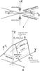 |
Fig. 1 Schematic view of the system. Top panel: scheme of the reconnection region. Bottom panel: 3D sketch of the dipolarization front configuration with the main parameters indicated. |
In this paper, we consider ion acceleration related to particle interaction with the
dipolarization front in the reconnection outflow regions. A schematic view of the
configuration of magnetic fields is shown in Fig. 1. We
suggest formation of fronts in the reconnection region and subsequent propagation in the
outflow region. There are several mechanisms, which can be responsible for particle
acceleration in such system. First of all, particles with thermal velocities around the
velocity of front propagation vφ can be
reflected from the front with the corresponding energy gain (e.g., Zhou et al. 2010; Ukhorskiy et al.
2014). Such a reflection corresponds to a nonadiabatic energy increase
 , where
m is a particle mass (that is similar to ion drift acceleration at shock
waves (Decker & Vlahos 1985; Zank et al. 1996; Gedalin 1996) and in current sheets, e.g., Lyons
& Speiser 1982). Thus, acceleration due to reflection is more effective for
heavy ions (Zimbardo 2010, 2011; Nisticò & Zimbardo
2012). However, it is unclear how the energy gain depends on particle mass for
multiple reflections from the front. We consider this question below. Particles with small
initial thermal velocities interact with the front in the adiabatic regime. In this case,
one can introduce the adiabatic invariant, which helps to describe particle acceleration.
, where
m is a particle mass (that is similar to ion drift acceleration at shock
waves (Decker & Vlahos 1985; Zank et al. 1996; Gedalin 1996) and in current sheets, e.g., Lyons
& Speiser 1982). Thus, acceleration due to reflection is more effective for
heavy ions (Zimbardo 2010, 2011; Nisticò & Zimbardo
2012). However, it is unclear how the energy gain depends on particle mass for
multiple reflections from the front. We consider this question below. Particles with small
initial thermal velocities interact with the front in the adiabatic regime. In this case,
one can introduce the adiabatic invariant, which helps to describe particle acceleration.
Nonadiabatic particle interaction with the front can have a resonant character. In this case, particles are captured by the front and gain energy stably due to motion along the front. One of the possibilities of this resonant interaction corresponds to the electrostatic field occurring in the vicinity of the front. A gradient of the magnetic field at the front results in the separation of ion and electron motions and leads to formation of strong transverse electrostatic fields found in numerical simulations (e.g., Sitnov & Swisdak 2011) and in spacecraft observations in the Earth magnetosphere (Runov et al. 2011; Khotyaintsev et al. 2011; Fu et al. 2012). The effect of this electrostatic field on particle acceleration is well known for shock waves where it is responsible for surfatron acceleration (e.g., Sagdeev 1966; Lee et al. 1996). For sufficiently thin fronts, the surfatron acceleration can be substantially more effective in comparison with the drift mechanism of acceleration (Lever et al. 2001).
The second opportunity corresponds to the distribution of the main component of the magnetic field. In contrast to shock waves, where the magnetic field does not change the sign, in the vicinity of the front, strong currents of trapped ions can create a localized region with a reversed magnetic field (see examples of observation in the Earth and Jupiter magnetospheres, Runov et al. 2011; Kasahara et al. 2013). This feature of the magnetic field configuration makes it possible to capture charge particles and accelerate them along the front (Takeuchi 2005; Artemyev et al. 2012; Ukhorskiy et al. 2014).
The third mechanism responsible for resonant acceleration corresponds to evolution of the front structure in the course of propagation. The front can slow down due to propagation toward the region with increased magnetic field (Nakamura et al. 2009; Panov et al. 2010; Birn et al. 2011). Effects of such front evolution on particle acceleration were not considered before. In this paper, we investigate the possible dependence of efficiency of all these resonant mechanisms on the particle mass and electric charge.
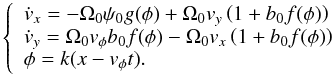
2. Ion interaction with the dipolarization front
The equations of motion of a particle with charge q and mass
m in the system shown in Fig. 1 can
be written as ![\begin{equation} \left\{ \begin{array}{l} \dot v_x = \Omega _0 v_y \left( {1 + b_0 f(\phi )} \right) \\ [0.5mm] \dot v_y = \Omega _0 v_\phi b_0 f(\phi ) - \Omega _0 v_x \left( {1 + b_0 f(\phi )} \right) \\ [0.5mm] \phi = (x - v_\phi t)/L, \\ \end{array} \right. \label{eq:motion} \end{equation}](/articles/aa/full_html/2014/02/aa22462-13/aa22462-13-eq14.png) (1)where
L is the front thickness, vφ
is the front velocity,
Ω0 = qBz/mc,
Bz is the amplitude of the background field,
and
b0 = B0/Bz
with B0 the peak amplitude of the front field, while the
function f(φ) describes the field profile across the front
and the motional electric field along the y direction is given by
Ey = −vφBzb0f(φ)/c.
We introduce the initial amplitude of a particle velocity, v0,
and the parameter k = 1/L (i.e.
φ = k(x − vφt)).
We assume that the background magnetic field Bz
is small and, as a result, the corresponding Larmor radius
ρ0 = v0/Ω0
is large, while the Larmor frequency Ω0 is small. In this case, two systems can
be considered: the slow moving relatively thick front
(kρ0 ~ 1,
vφ ≪ v0) and
the fast moving thin front (kρ0 ≫ 1,
vφ ~ v0). The
latter system cannot be described analytically. To obtain qualitative information about
particle acceleration in such system, we, thus, use numerical calculations of test particle
trajectories. We find the maximum possible gain of energy
ε∗ = (1/2)maxv2
(where
(1)where
L is the front thickness, vφ
is the front velocity,
Ω0 = qBz/mc,
Bz is the amplitude of the background field,
and
b0 = B0/Bz
with B0 the peak amplitude of the front field, while the
function f(φ) describes the field profile across the front
and the motional electric field along the y direction is given by
Ey = −vφBzb0f(φ)/c.
We introduce the initial amplitude of a particle velocity, v0,
and the parameter k = 1/L (i.e.
φ = k(x − vφt)).
We assume that the background magnetic field Bz
is small and, as a result, the corresponding Larmor radius
ρ0 = v0/Ω0
is large, while the Larmor frequency Ω0 is small. In this case, two systems can
be considered: the slow moving relatively thick front
(kρ0 ~ 1,
vφ ≪ v0) and
the fast moving thin front (kρ0 ≫ 1,
vφ ~ v0). The
latter system cannot be described analytically. To obtain qualitative information about
particle acceleration in such system, we, thus, use numerical calculations of test particle
trajectories. We find the maximum possible gain of energy
ε∗ = (1/2)maxv2
(where  ) and the dependencies
of ε∗ on the system parameters.
) and the dependencies
of ε∗ on the system parameters.
In the first part of this paper, we use a simplified model to describe particle interaction with fronts. We neglect the influence of the normal (i.e., along x) electrostatic fields (the effects of these fields are described in Sect. 3.1). We consider the system where the magnetic field is always positive 1 + b0f(φ) > 0 (effects of magnetic field zeros are described in Sect. 3.2). We assume that the structure of the front does not change during time interval of particle interaction with the front (effects of front evolution are considered in Sect. 3.3). The possible influence of Bx ≠ 0 and By ≠ 0 is also discussed in Sect. 4.
To carry out all estimates, we use the simplified function f(φ) = (1/2)(a − tanh(φ))exp(−(φ/σ)2). Here, the parameter σ regulates the scale of the entire structure of the front (see Fig. 1), while varying the value of the parameter a allows us to define a small minimum of the magnetic field before the front. Profiles of dimensionless magnetic field 1 + b0f(φ) for three values of a are shown in Fig. 2.
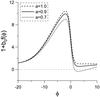 |
Fig. 2 Profiles of the magnetic field 1 + b0f(φ) with σ = 10, b0 = 15. |
2.1. Systems with kρ0 ≫ 1
In the systems with kρ0 ≫ 1, particles
interact with the front in the nonadiabatic regime, when the time of particle interaction
is substantially smaller than a Larmor period of oscillations ahead the front. The example
of the numerical solution of system of Eq. (1) is shown in Fig. 3. The particle
trajectory consists on four fragments: the initial Larmor rotation, acceleration due to
motion along the front (motion ahead the front for this fragment is shown by gray color),
loss of energy after front crossing, and the final Larmor rotation. The energy increase
due to the motion along Ey is almost
compensated by the energy loss when returning back. However, some difference of initial
and final energies can be found due to nonadiabatic scattering of particles at the front.
For example, the difference between initial and final energies is about
 for the trajectory
from Fig. 3. In this case, a substantial energy gain
is possible considering the finite size of the front along the y
direction. If particles reach the front boundary before crossing the front, then all of
the gained energy, ε∗ (see Fig. 3), is retained.
for the trajectory
from Fig. 3. In this case, a substantial energy gain
is possible considering the finite size of the front along the y
direction. If particles reach the front boundary before crossing the front, then all of
the gained energy, ε∗ (see Fig. 3), is retained.
The particle interaction with the front before the crossing can be considered as
successive particle reflections from the front. Each reflection consists on two parts: a
half of Larmor rotation ahead the front and other half of Larmor rotation behind the
front. Both these two parts corresponds to gain of energy. The electric field behind the
front (~b0) is substantially stronger than the electric field
ahead the front and, as a result, the main gain of energy corresponds to particle motion
behind the front in the +y direction (a second half of Larmor rotation).
For a single reflection, this energy gain can be estimated as
 (i.e.,
particles pass a distance around
~2v/(Ω0b0)
along the electric field
~vφΩ0b0).
This gain corresponds to the classical mechanism of acceleration of particles reflected
from a moving wall (e.g., Shabansky 1971; Lyons & Speiser 1982).
(i.e.,
particles pass a distance around
~2v/(Ω0b0)
along the electric field
~vφΩ0b0).
This gain corresponds to the classical mechanism of acceleration of particles reflected
from a moving wall (e.g., Shabansky 1971; Lyons & Speiser 1982).
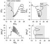 |
Fig. 3 Particle trajectory and corresponding energy as a function of time. System parameters are kρ0 = 10, vφ/v0 = 1, b0 = 15. Top left panel: projection of the particle trajectory onto (x,y) plane. The region of particle acceleration before the front crossing is shown by the gray color. We also indicate the initial and final positions of the particle characterized by corresponding Larmor circles. Bottom left panel: particle energy as a function of time. The value of energy ε∗ before particle crossing of the front is indicated. Two right panels show the particle coordinate along the front and the particle energy as functions of the wave-phase. These two panels clearly demonstrate particle motion before (gray color) and after front crossing. |
The parameters (k, b0, vφ) determine the maximum number of particle reflections from the front and, as a result, can determine the final gain of energy ε∗. To check these dependencies we find trajectories with the maximum possible ε∗ in systems with various k and vφ (see Fig. 4). For this reason we run 104 particles and define ε∗ for each particle trajectory. The final energy gain is almost independent on kρ0 as well as on vφ/v0. The exception is only systems with small vφ/v0 (such systems are considered below separately). With the increase in vφ, the energy gain for a single reflection from the front grows, but the number of such reflections decreases. The thickness of the front 1/k (if it is small enough) does not influence the particle interaction with the front.
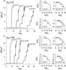 |
Fig. 4 Particle trajectories and corresponding energies as functions of time for systems with two values of kρ0 and four values of vφ (b0 = 15). Only the parts of trajectories before front crossing are shown. Trajectories are shown in eight separated small panels, while energies as functions of time are presented in two panels for two different kρ0 values. For each trajectory the corresponding value of vφ/v0 is indicated inside the panels. |
Figure 5 shows trajectories with the maximum ε∗ for various values of b0. The final energy gain is almost linearly proportional to b0 (as it should be for adiabatic interaction). The nonadiabatic effect corresponds to energy quantization regarding a single reflection. For b0 < 10, we have only one reflection; for 10 < b0 < 17, there are two reflections and so on. However, the final energy increases with b0 as ε∗ ~ b0.
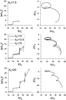 |
Fig. 5 Particle trajectories and corresponding energies as functions of time. System parameters are kρ0 = 10 and vφ/v0 = 1. Only the parts of trajectories before front crossing are shown. The right panels show five trajectories calculated for five different b0 values. Corresponding dependencies of particle energies on time before front crossings are shown in the left panels. |
2.2. Systems with kρ0 ~ 1 and vφ ≪ v0
In the case of small velocity of the dipolarization front,
vφ ≪ v0, we
deal with the classical system with one degree of freedom and a slow time
τ = kvφt.
The dimensionless Hamiltonian of this system can be written as
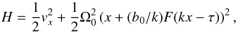 where
F = ∫f(φ)dφ.
The phase portrait of this system with a frozen time τ is shown in Fig.
6a. The changing of τ corresponds
to a modification of the effective potential where particles oscillate. Because
dτ/dt ≪ d(x/ρ0)/dt
and the particle motion is periodic, we can introduce the adiabatic invariant (Landau & Lifshitz 1988),
where
F = ∫f(φ)dφ.
The phase portrait of this system with a frozen time τ is shown in Fig.
6a. The changing of τ corresponds
to a modification of the effective potential where particles oscillate. Because
dτ/dt ≪ d(x/ρ0)/dt
and the particle motion is periodic, we can introduce the adiabatic invariant (Landau & Lifshitz 1988),
 Conservation
of this invariant results in a relation between the particle energy H and
the slow time τ. We plot
I(H,τ) = const. in Fig. 6b. One can see that the total variation of the particle
energy is zero (particles start and finish with the same energies). However, the particle
energy in the middle of the way can be substantially larger than the initial value.
Therefore, if particles reach the boundary of the front along the y-axis
before the crossing of the entire front, they can gain a certain energy.
Conservation
of this invariant results in a relation between the particle energy H and
the slow time τ. We plot
I(H,τ) = const. in Fig. 6b. One can see that the total variation of the particle
energy is zero (particles start and finish with the same energies). However, the particle
energy in the middle of the way can be substantially larger than the initial value.
Therefore, if particles reach the boundary of the front along the y-axis
before the crossing of the entire front, they can gain a certain energy.
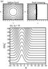 |
Fig. 6 Panel a) phase portraits before the front crossing and during the crossing. Panel b) counters I(H,τ) = const. |
The results shown in Fig. 6 are compared with numerical calculation of Hamiltonian equations (see Fig. 7). One can see that the form of energy dependence on time is identical with our analytical estimates. As it should be for adiabatic systems, the energy variation is proportional to the variation in the magnetic field.
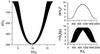 |
Fig. 7 Particle trajectory and corresponding energy as a function of time. Right bottom panel: magnetic field along the trajectory. |
3. Resonant acceleration
Both the configuration of the front magnetic field and the peculiarities of front evolution
can result in a resonance regime of acceleration when the particles move with the front
(i.e., on average  ).
This acceleration mechanism resembles the surfatron acceleration of charged particles by
strong electrostatic wave (see Katsouleas & Dawson
1983) when particles are trapped in the vicinity of the wave-front. In this
section, we consider three possible realizations of such resonant acceleration of ions.
).
This acceleration mechanism resembles the surfatron acceleration of charged particles by
strong electrostatic wave (see Katsouleas & Dawson
1983) when particles are trapped in the vicinity of the wave-front. In this
section, we consider three possible realizations of such resonant acceleration of ions.
3.1. Surfatron acceleration: effect of Ex
Here we describe the effect of the electrostatic field
Ex on particle acceleration. This field
can be considered as a classical Hall field, which appears due to separation of ion and
electron motions in the vicinity of the front. To describe the shape of
Ex, we write force balance for electrons
(Shkarofsky et al. 1966) in the front (we neglect
the inertia terms ~me), ![\begin{eqnarray*} \nabla p_{\rm e} = - en_{\rm e} E_x + c^{ - 1} \left[ {{\vec j}_{\rm e} \times {\vec e}_z } \right]B_0 f(\phi ), \end{eqnarray*}](/articles/aa/full_html/2014/02/aa22462-13/aa22462-13-eq83.png) where
pe is the electron pressure, ne
is the electron density, and je is the electron current density.
We assume that the term ∇pe is small enough (this assumption
is supported by spacecraft observations of dipolarization fronts in the Earth
magnetosphere, see Fu et al. 2012), and the
electron current can be estimated as
je = −χey(c/4π)∂(B·ez)/∂x = −χey(c/4πL)B0df(φ)/dφ,
where the coefficient χ ≤ 1 determines a contribution of electrons to the
total current density. In this case, we have
where
pe is the electron pressure, ne
is the electron density, and je is the electron current density.
We assume that the term ∇pe is small enough (this assumption
is supported by spacecraft observations of dipolarization fronts in the Earth
magnetosphere, see Fu et al. 2012), and the
electron current can be estimated as
je = −χey(c/4π)∂(B·ez)/∂x = −χey(c/4πL)B0df(φ)/dφ,
where the coefficient χ ≤ 1 determines a contribution of electrons to the
total current density. In this case, we have 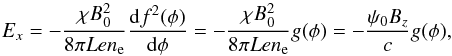 where
we introduce the constant speed of current carrying electrons
ψ0. We write equations of ion motion as
where
we introduce the constant speed of current carrying electrons
ψ0. We write equations of ion motion as
 The
presence of Ex can result in the particle
being captured by the front (e.g., Lee et al.
1996). In this case particles move with the front and
The
presence of Ex can result in the particle
being captured by the front (e.g., Lee et al.
1996). In this case particles move with the front and
 (i.e.
vx = vφ):
(i.e.
vx = vφ):
 The
first equation corresponds to the Hamiltonian system
The
first equation corresponds to the Hamiltonian system 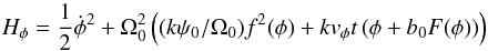 where
F(φ) = ∫f(φ)dφ.
The effective potential of this system
where
F(φ) = ∫f(φ)dφ.
The effective potential of this system  is shown in Fig. 8. One can see that the electric
field creates a small potential well ahead the front
(φ > 0). This well disappears when
kvφt
becomes large enough. The maximum possible time interval Δt, which
particles spend in this resonant regime, can be found from the simple equation
is shown in Fig. 8. One can see that the electric
field creates a small potential well ahead the front
(φ > 0). This well disappears when
kvφt
becomes large enough. The maximum possible time interval Δt, which
particles spend in this resonant regime, can be found from the simple equation
 ;
that is, particles should be escaped from the resonance when the first term
Ω0ψ0g(φ) ~ 2Ω0ψ0f(φ)df/dφ
becomes equal (or smaller) than the second term
Ω0vy(1 + b0f(φ)) ~ Ω0vyb0f(φ)
where
vy ~ vφΩ0Δt:
;
that is, particles should be escaped from the resonance when the first term
Ω0ψ0g(φ) ~ 2Ω0ψ0f(φ)df/dφ
becomes equal (or smaller) than the second term
Ω0vy(1 + b0f(φ)) ~ Ω0vyb0f(φ)
where
vy ~ vφΩ0Δt:
 An
example of particle motion and acceleration in this regime is shown in Fig. 9. The particle oscillates around the Larmor trajectory
and then becomes trapped by the front. In contrast to the trajectories shown in Figs.
3 and 4 the
trapped particle does not cross the front in the course of acceleration. The corresponding
phase φ calculated along the trajectory oscillates around a constant
value (
An
example of particle motion and acceleration in this regime is shown in Fig. 9. The particle oscillates around the Larmor trajectory
and then becomes trapped by the front. In contrast to the trajectories shown in Figs.
3 and 4 the
trapped particle does not cross the front in the course of acceleration. The corresponding
phase φ calculated along the trajectory oscillates around a constant
value ( ).
).
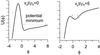 |
Fig. 8 Effective potential of the system for two moments of time. |
 |
Fig. 9 Particle trajectory. Grey color shows motion in capture. System parameters are kρ0 = 100, b0 = 15, vφ/v0 = 0.5, and ψ0 = kρ0. Two top panels: projections of the particle trajectory onto the (x,y) plane and (vx,vy) plane. Bottom panels: evolution of wave-phase along the trajectory and the particle energy as a function of time. |
3.2. Surfatron acceleration: effect of zero of Bz
Here, we discuss the effect of a local zero of the magnetic field. If the front is strong
enough, the sum of the front and background magnetic fields can change the sign in the
vicinity of the front (see an example in Fig. 2; see
also in situ measurements of the magnetic field reported by Runov et al. 2011). For a such configuration, one can find the solution
of the equation
1 + b0f(φ) = 0. This
situation is similar to the one considered in Sect. 3.1. However, we have another system for the fast phase φ in
the vicinity of the resonance  in this case:
 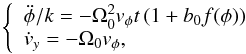 where
1 + b0f(φ) oscillates
around zero. The corresponding profiles of the effective potential are shown in Fig. 10. One can see that the local minimum of the potential
always exists. Therefore, particles cannot leave this regime of acceleration. An example
of the corresponding trajectory is shown in Fig. 11.
Trapping in the vicinity of the magnetic field zero results in meandering oscillations in
the (x,y) plane (compare with Artemyev et
al. 2012). Also, the wave phase φ calculated along the
trajectory oscillates around constant value.
where
1 + b0f(φ) oscillates
around zero. The corresponding profiles of the effective potential are shown in Fig. 10. One can see that the local minimum of the potential
always exists. Therefore, particles cannot leave this regime of acceleration. An example
of the corresponding trajectory is shown in Fig. 11.
Trapping in the vicinity of the magnetic field zero results in meandering oscillations in
the (x,y) plane (compare with Artemyev et
al. 2012). Also, the wave phase φ calculated along the
trajectory oscillates around constant value.
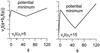 |
Fig. 10 Effective potentials of the system for two moments of time. |
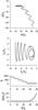 |
Fig. 11 Particle trajectory in the system with the local zero of the magnetic field. System parameters are kρ0 = 100, b0 = 15, vφ/v0 = 0.5, and a = 0.7. Two top panels: projections of the particle trajectory onto (x,y) plane and (vx,vy) plane. Bottom panels: evolution of wave-phase along the trajectory and the particle energy as a function of time. |
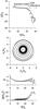 |
Fig. 12 Particle trajectory in the system with |

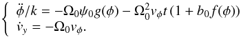
3.3. Surfatron acceleration: effect of nonstationarity of the front
Here we consider the effects of nonstationarity of the front. To model the variation of
front velocity, we introduce the function ℓ(x) and use
the following expression for a dimensionless phase
φ = k(∫ℓ(x′)dx′ − vφt).
In this case, the effective front velocity is  .
Thus, the front propagates with the inhomogeneous velocity. We should mention that the
front profile f(φ) can be used for this nonstationary
system only until a certain moment tb. In the course of front
evolution (when the front slows down), the profile f(φ)
becomes more sharp and after tb the front should break. Thus,
we consider the front resonant interaction with particles for a time interval before front
breaking. The corresponding equations of motion take the form
.
Thus, the front propagates with the inhomogeneous velocity. We should mention that the
front profile f(φ) can be used for this nonstationary
system only until a certain moment tb. In the course of front
evolution (when the front slows down), the profile f(φ)
becomes more sharp and after tb the front should break. Thus,
we consider the front resonant interaction with particles for a time interval before front
breaking. The corresponding equations of motion take the form
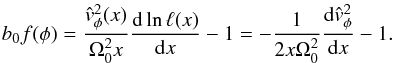
![\begin{eqnarray*} \left\{ \begin{array}{l} \dot v_x = \Omega_0v_y \left( {1 + b_0 f(\phi )} \right) \\ [2mm] \dot v_y = \Omega_0\hat v_\phi (x)b_0 f(\phi ) - \Omega_0v_x \left( {1 + b_0 f(\phi )} \right). \\ \end{array} \right. \end{eqnarray*}](/articles/aa/full_html/2014/02/aa22462-13/aa22462-13-eq127.png) We
consider the resonant condition
We
consider the resonant condition  :
:
![\begin{eqnarray*} \left\{ \begin{array}{l} \ddot \phi /k = {\displaystyle \frac{{{\rm d}\ell (x)}}{{{\rm d}x}}} \hat v_\phi ^2 (x) + \Omega_0v_y\ell(x) \left( {1 + b_0 f(\phi )} \right) \\[2mm] \dot v_y = - \Omega_0\hat v_\phi (x). \\ \end{array} \right. \end{eqnarray*}](/articles/aa/full_html/2014/02/aa22462-13/aa22462-13-eq129.png) For
resonant acceleration of particles, the right side of the first equation should have a
point of stationary phase (i.e., some value of φ when
For
resonant acceleration of particles, the right side of the first equation should have a
point of stationary phase (i.e., some value of φ when
 ). Therefore, we have
 If
dℓ(x)/dx > 0
(i.e. the front slows down
If
dℓ(x)/dx > 0
(i.e. the front slows down  ),
this condition can be satisfied. For example, if
ℓ(x) = (x/l0)α,
then the inequality
b0f(φ) = α(vφ/l0Ω0)2(x/l0)− 2−2α−1 > 0
is satisfied for small enough x. In this case, particles can be trapped
by the front and move with it. The example of such a trajectory is shown in Fig. 12. The characteristic time interval
Δt, which particles can spend in this resonant regime, is defined by the
equation
α(vφ/l0Ω0)2(δx/l0)− 2−2α ≈ 1
where
δx = vφΔt.
),
this condition can be satisfied. For example, if
ℓ(x) = (x/l0)α,
then the inequality
b0f(φ) = α(vφ/l0Ω0)2(x/l0)− 2−2α−1 > 0
is satisfied for small enough x. In this case, particles can be trapped
by the front and move with it. The example of such a trajectory is shown in Fig. 12. The characteristic time interval
Δt, which particles can spend in this resonant regime, is defined by the
equation
α(vφ/l0Ω0)2(δx/l0)− 2−2α ≈ 1
where
δx = vφΔt.
Comparison of acceleration mechanisms for systems with δy < Δy.
4. Discussion
In this paper, we considered several mechanisms responsible for particle acceleration by
reconnection outflow jets. The most natural and simple mechanism corresponds to the drift
nonadiabatic acceleration due to multiple reflections of particles from the front. This
mechanism provides energy gain proportional to the particle mass and, as a result, heavy
ions are accelerated more effectively than protons. In contrast to the classical drift
acceleration in the shock-waves (see review by Decker
& Vlahos 1985) where only one-two reflections are possible, the large
magnetic field amplitude and slow propagation of dipolarization fronts allow for multiple
reflections. However, the presence of the reversed gradient of the magnetic field behind the
front results in an energy loss: the total energy gain for nonadiabatic particles crossing
the front cannot exceed a value corresponding to the single reflection. Larger energy gain
is possible if particles escape the close vicinity of the front due to a finite front width
along y direction. In the most optimistic scenario, particles can save all
the gained energy, which substantially exceeds the energy corresponding to the single
reflection. Thus, the width of the front is a critical parameter of the system for ion
acceleration. A typical path δy passed by particles before front crossing
can be estimated as  where
v0 is the amplitude of the initial particle velocity, and we
use the expressions
(v/v0)2 ~ b0
and
Ey ~ (vφ/c)B0.
Both dependencies,
δy ~ 1/vφ
and δy ~ b0, can be found in Figs. 4 and 5. If the width
of the front Δy is much larger than δy, then only a small
population of accelerated particles can escape the close vicinity of the front with the
gained energy. In the opposite case, Δy ≪ δy, no one
particle can gain the maximum possible energy. Thus, the optimal relation is
Δy ~ δy where all particles gain some energy and escape
the front before crossing it along x. For the nonadiabatic regime of
acceleration,
vφ ~ v0, we need
Δy ~ b0ρ0.
where
v0 is the amplitude of the initial particle velocity, and we
use the expressions
(v/v0)2 ~ b0
and
Ey ~ (vφ/c)B0.
Both dependencies,
δy ~ 1/vφ
and δy ~ b0, can be found in Figs. 4 and 5. If the width
of the front Δy is much larger than δy, then only a small
population of accelerated particles can escape the close vicinity of the front with the
gained energy. In the opposite case, Δy ≪ δy, no one
particle can gain the maximum possible energy. Thus, the optimal relation is
Δy ~ δy where all particles gain some energy and escape
the front before crossing it along x. For the nonadiabatic regime of
acceleration,
vφ ~ v0, we need
Δy ~ b0ρ0.
According to the direct spacecraft observation in the Earth magnetosphere the width Δy of fronts is associated with an initial scale of the reconnection region (for the Earth’s magnetosphere the width of fronts is about ~104 km, see Nakamura et al. 2004, 2009). If we assume that the same relation between spatial scales is valid in the solar corona current sheet, then Δy can be estimated as ~102−104 km from numerical modeling (e.g. Aulanier et al. 2013) and observations (e.g. Ciaravella & Raymond 2008; Liu et al. 2010). In the solar corona, polar jets observed in the X-ray by the Yohkoh spacecraft have lengths of 104–4 × 10⁵ km, widths of 5 × 10³–105 km, and speeds ranging from 10 to 1000 km s-1 (Shimojo et al. 1996). Also, a selection of jets, which are visible both in the coronograph and in the UV by STEREO, have lifetimes of 20–30 min and typical speeds of 270–400 km s-1 (Nisticò et al. 2009). Hence, jets are subalfvenic in the majority of cases. For the present study, we can assume that the width of the jet front is on the same order of the observed jet width, 5 × 10³–105 km, and speeds on the order of 200–400 km s-1. We can argue that small reconnection events in the corona can correspond to smaller jet front widths.
Taking into account values of the magnetic field and plasma temperature in the solar corona (e.g., Reeves et al. 2008), we estimate the Larmor radius for oxygen ions as 10–100 m. Therefore, the relation Δy ~ b0ρ0 < 1 km cannot be satisfied. Thus, particles can escape the close vicinity of the front with all gained energy before a front crossing, only if these particles are initially located in the vicinity of the front boundary. However, this situation can be changed in the case of resonant interaction.
For all three resonance mechanisms, which can be realized at the front, the maximum energy gain depends on two different factors. First of all, the maximum energy gain is defined by the front width. If particles escape from the resonant interaction in the boundary of the front, then their energy is about qEyΔy, where Δy is the front width and Ey ~ (vφ/c)B0. This energy gain does not depend on the particle mass (as it should be for the ballistic acceleration by a constant electric field), but it depends on particle charge q. However, particle resonant interaction with fronts is also limited by a time interval when the corresponding resonant mechanism can be involved. This time interval Δt is defined by the resonance conditions. For surfatron acceleration caused by the electrostatic field Ex ~ Bzψ0/c one can estimate ΔtΩ0 ~ ψ0/vφ. The surfatron acceleration in the case of inhomogeneity of the front velocity vφ ~ (l0/x)α corresponds to the time interval ΔtΩ0 ~ (Ω0l0/vφ)α/(1 + α), where l0 is the scale of inhomogeneity (for α < 1 we have 2α/(1 + α) < 1). Therefore, the corresponding energy gain ~m(vφΔtΩ0)2 is larger for heavy ions for these two mechanisms (see Table 1).
Due to the large front width, Δy, in comparison with
ρ0, almost all particles are able to gain the maximum possible
energy for the first resonant mechanism related to
Ex field, where the time interval of resonant
interaction is smaller than the time necessary to pass the distance Δy.
Thus, this mechanism is responsible for particle acceleration in the vicinity of the front
boundary when the accelerated particles escape from the front before the front crossing. The
typical energy, which can be provided by this mechanism, is
 , where we
assume L ~ ρ0 and introduce
vA ~ vφ ~ 200
km s-1. For b0 ~ 10–15, this energy gain is
substantially larger than the energy gain due to multireflections
, where we
assume L ~ ρ0 and introduce
vA ~ vφ ~ 200
km s-1. For b0 ~ 10–15, this energy gain is
substantially larger than the energy gain due to multireflections
 .
.
The surfatron acceleration due to inhomogeneity of the front velocity can be responsible
for the energy gain up to  , where
r = Ω0l0/vφ.
The scale of the front inhomogeneity l0 is about the distance
between an initial magnetic loop and the reconnection region
Δx ~ 104–106 km. As a result, the corresponding
parameter
r2α/(1 + α)
is larger than 50 even for weak inhomogeneity α ~ 0.1–0.2. Thus, the energy
gain due to this resonant mechanism can be substantially larger than the energy gain
provided by multireflection. The corresponding condition for gain of the maximum possible
energy is
Δy > l0r(1 − α)/(1 + α).
This condition can be satisfied already for
l0 ~ Δx/10 (these
estimates are reasonable, see simulations by Birn et al.
2011). However, we should mention here that the maximum energy gain is determined
by Δy for α ~ 1 and is proportional to particle charge.
, where
r = Ω0l0/vφ.
The scale of the front inhomogeneity l0 is about the distance
between an initial magnetic loop and the reconnection region
Δx ~ 104–106 km. As a result, the corresponding
parameter
r2α/(1 + α)
is larger than 50 even for weak inhomogeneity α ~ 0.1–0.2. Thus, the energy
gain due to this resonant mechanism can be substantially larger than the energy gain
provided by multireflection. The corresponding condition for gain of the maximum possible
energy is
Δy > l0r(1 − α)/(1 + α).
This condition can be satisfied already for
l0 ~ Δx/10 (these
estimates are reasonable, see simulations by Birn et al.
2011). However, we should mention here that the maximum energy gain is determined
by Δy for α ~ 1 and is proportional to particle charge.
For surfatron acceleration of particles that are captured in the vicinity of the magnetic
field reversal, a time interval ΔtΩ0 is defined by the
configuration of the background magnetic field. First of all, particles need
 to reach the front boundary along y-direction. In this case, the final
energy gain is about
qEyΔy. On
the other hand, there is an increase in the magnitude of the background magnetic field along
the direction of the front propagation in the realistic magnetic field configuration. Thus,
there exists some region, where the sum of the front magnetic field and background magnetic
field, cannot be equal to zero. The particles, which are captured, can be accelerated, while
the front passes a certain distance Δx between the initial moment of
capture and the moment of the disappearance of the zero magnetic field region. The
corresponding time interval
Δtx = Δx/vφ
does not depend on the particle mass. As a result, the final energy gain is
~m(vφΩ0Δtx)2 = m(Ω0Δx)2 ~ q2/m.
The latter estimates are valid for systems with
Δtx < Δty,
or
Δy > 0.5Ω0(Δx)2/vφ.
The scale Δx can be defined as a distance between the reconnection region
and the initial magnetic loop, where the background magnetic field is strong enough. As a
result, we obtain a similar condition as conditions for the resonant mechanism that
corresponds to the front inhomogeneity. However, such long-time acceleration requires the
absence of any magnetic field fluctuations, which can destroy the resonance. Below, we
discuss the corresponding effect of such fluctuations.
to reach the front boundary along y-direction. In this case, the final
energy gain is about
qEyΔy. On
the other hand, there is an increase in the magnitude of the background magnetic field along
the direction of the front propagation in the realistic magnetic field configuration. Thus,
there exists some region, where the sum of the front magnetic field and background magnetic
field, cannot be equal to zero. The particles, which are captured, can be accelerated, while
the front passes a certain distance Δx between the initial moment of
capture and the moment of the disappearance of the zero magnetic field region. The
corresponding time interval
Δtx = Δx/vφ
does not depend on the particle mass. As a result, the final energy gain is
~m(vφΩ0Δtx)2 = m(Ω0Δx)2 ~ q2/m.
The latter estimates are valid for systems with
Δtx < Δty,
or
Δy > 0.5Ω0(Δx)2/vφ.
The scale Δx can be defined as a distance between the reconnection region
and the initial magnetic loop, where the background magnetic field is strong enough. As a
result, we obtain a similar condition as conditions for the resonant mechanism that
corresponds to the front inhomogeneity. However, such long-time acceleration requires the
absence of any magnetic field fluctuations, which can destroy the resonance. Below, we
discuss the corresponding effect of such fluctuations.
On the basis of our analysis, we can define different regions, where different mechanisms of ion acceleration are involved (see Fig. 13). In the vicinity of the reconnection region, a depression of the background magnetic field Bz can lead to the realization of surfatron acceleration in the localized magnetic field zero. In contrast, a gradient of the background magnetic field can run resonant acceleration via dvφ/dx ≠ 0 at some distance from the X-line. During the whole interval of front travelling, ions can gain energy due to multireflection and resonant acceleration provided by Ex ≠ 0 at the front edge.
 |
Fig. 13 Schematic view of localization of various mechanisms of particle acceleration. |
Here we also should mention the possible role of magnetic field fluctuations. The magnetic
reconnection in the solar corona can include electromagnetic turbulence with corresponding
particle heating by random fields (see review by Petrosian
2012). These field fluctuations can be convected away from the reconnection region
by dipolarization fronts. In this case, electromagnetic field fluctuations may have an
influence on particle acceleration by fronts. Moreover, a strong gradient of the magnetic
field in the vicinity of the front is responsible for the development of various plasma
instabilities, which create a broad spectrum of electromagnetic fluctuations observed by
spacecraft in the Earth magnetotail (e.g., Zimbardo et al.
2010; Khotyaintsev et al. 2011; Panov et al. 2013). Thus, we should consider the
influence of these fluctuations on ion acceleration (see, for instance, Perri et al. 2011). For the classical drift acceleration
in the shock fronts, the effect of magnetic field fluctuations provided by Alfvén waves was
studied by Decker et al. (1984); Decker & Vlahos (1985). It was shown that the
strong wave activity helps particles to cross the shock-front several times and increase the
final energy gain. For the resonant surfatron acceleration, magnetic field fluctuations play
another role. The presence of small-scale fast fluctuations results in destruction of the
resonance, and the final energy gain can be decreased. The time, which is necessary for
resonance destruction, is proportional to  ,
where Pw is the spectral density of magnetic
field fluctuations measured in nT2/Hz (Artemyev et
al. 2011). Thus, particles can gain substantially energy for weak enough wave
activity. On the other hand, if particles spend a long enough time in resonance (as for
surfatron acceleration in the vicinity of the magnetic field reversal), magnetic field
fluctuations really limit the maximum gained energy. Artemyev
et al. (2011) showed that the maximum possible energy of particles accelerated in
the vicinity of the magnetic field reversal in presence of fluctuations is
,
where Pw is the spectral density of magnetic
field fluctuations measured in nT2/Hz (Artemyev et
al. 2011). Thus, particles can gain substantially energy for weak enough wave
activity. On the other hand, if particles spend a long enough time in resonance (as for
surfatron acceleration in the vicinity of the magnetic field reversal), magnetic field
fluctuations really limit the maximum gained energy. Artemyev
et al. (2011) showed that the maximum possible energy of particles accelerated in
the vicinity of the magnetic field reversal in presence of fluctuations is
 . This estimate is valid for
systems with
. This estimate is valid for
systems with  .
For magnetic field fluctuations observed in the Earth magnetotail (see Zimbardo et al. 2010), we can rewrite this condition as
Δx > 104 km. Thus, the acceleration of
particles in the vicinity of the magnetic field reversal for realistic magnetic field
configuration should be bounded by magnetic field fluctuations. In this case, we have the
gain
.
For magnetic field fluctuations observed in the Earth magnetotail (see Zimbardo et al. 2010), we can rewrite this condition as
Δx > 104 km. Thus, the acceleration of
particles in the vicinity of the magnetic field reversal for realistic magnetic field
configuration should be bounded by magnetic field fluctuations. In this case, we have the
gain  with
with
 instead of the gain ~m(Ω0Δx)2. To
have more accurate estimates, one needs to know precise information about the spectrum of
magnetic field fluctuations in the reconnected current sheet of the solar corona.
instead of the gain ~m(Ω0Δx)2. To
have more accurate estimates, one needs to know precise information about the spectrum of
magnetic field fluctuations in the reconnected current sheet of the solar corona.
In this paper, we have used a simplified 1D model of the dipolarization front. However, the efficiency of particle acceleration depends on a full 3D magnetic field configuration. Particulary, the curvature of the front surface determines the stability of particle acceleration in 2D systems (Bulanov & Sakharov 1986, 2000). The positive curvature provides the stable motion of captured particles. Indeed, spacecraft observations in the Earth magnetotail show that dipolarization fronts have positive curvature of the surface in the (x,z) plane (Runov et al. 2009). The configuration of the front magnetic field in the (x,z) plane is generally similar with the configuration of the magnetic field of a reconnected current sheet. As a result, trapped particles can move along the curved magnetic field lines. However, this motion does not result in escape from the resonance (see Vainchtein et al. 2005; Artemyev et al. 2013b). According to numerical modeling (e.g. Birn et al. 2013), the front curvature in the plane (x,y) is almost zero in the central region of the front, while the general front curvature in this plane is negative. This can decrease the efficiency of acceleration. Due to such front configuration, the effective width is about half the size of the total front width Δy.
We use a simplified model of the background magnetic field – only Bz component is taken into account. The 2D configuration of the reconnected current sheet includes Bx(z) components as well. Moreover, 3D reconnection often contains the guiding field component By (see reviews Yamada et al. 2010; Frank 2010, and references therein). The effect of these components on particle acceleration by dipolarization fronts can be important. The main current sheet component, Bx(z), reverses at the plane z = 0, and | Bx | grows with | z |. Thus, the particle motion is only slightly affected by Bx in the vicinity of this plane. There is a population of particles trapped in the vicinity of the z = 0 plane (e.g., Büchner & Zelenyi 1986). These particles spend a long time crossing z = 0 (so-called trapped and quasi-trapped orbits, see review Zelenyi et al. 2013, and references therein). Thus, trapped particles can be captured by the front and accelerated as described above. Moreover, it can be shown that the presence of Bx(z) does not stop the acceleration of these particles but can limit the maximum possible gain of energy (Artemyev et al. 2013b). The guiding component By is more ’dangerous’ for resonant acceleration. The presence of a finite By ≠ 0 substantially changes the charged particle motion in the current sheet and makes trajectories more complex (Artemyev et al. 2013c, and references therein). Gyration of particles in By component should destroy the resonant acceleration after a certain time interval (as when it happens for shock waves, see Lee et al. 1996). Thus, By can limit the possible energy gained by particles. Both these effects (Bx(z) and By) require a separated study.
The surfatron mechanism of acceleration is based on compensation of the Lorentz force corresponding to the background magnetic field ~vyBz by some force that corresponds to the front electromagnetic field. In the case of relativistic energies of particles, the Lorentz force is limited due to limitation of particle velocities (vyBz < cBz) and, as a result, surfatron acceleration is more stable and effective (Ucer & Shapiro 2001; Amano & Hoshino 2009). A force, which could compensate the Lorentz force, can be provided either by the electric field ~Ex, by the magnetic field of the front ~vyB0f(φ) as in case of f(φ) < 0, or by inhomogeneity of the front velocity. In the first case, we deal with the classical surfatron acceleration (Sagdeev & Shapiro 1973; Katsouleas & Dawson 1983), which is traditionally considered for electrostatic waves. However, as was shown by Cole (1976), the same effect of particle demagnetization due to compensation of the background Lorentz force can be obtained for any inhomogeneous electric field. This field can be provided by small-scale instabilities in the vicinity of the front (see examples of such systems in papers by Galeev et al. 1988; Balikhin et al. 1993) by separation of electron and ion motions (e.g., Gedalin 1996; Lee et al. 1996), or by interaction of two fronts (Roth & Bale 2006). Moreover, strongly inhomogeneous electrostatic fields in the vicinity of the reconnection region can also support surfatron acceleration of particles (Hoshino 2005; Artemyev et al. 2013a). Therefore, the obtained estimates of dependence of efficiency of acceleration on particle mass can be useful for other applications (not only for description of heavy ion acceleration in the solar corona).
It is interesting to note the difference between surfatron acceleration and direct
acceleration in the X-line. Both mechanisms deal with ballistic acceleration of particles
that moves along the constant electric field. However, the Lorentz force that corresponds to
the background magnetic field is compensated for acceleration along the front. Thus,
particle motion is stable. In contrast, acceleration in the X-line region is unstable, and
the corresponding particles trajectories should escape from the region of acceleration after
a certain time interval Δt (Bulanov
& Sasorov 1976; Galeev 1979; Zelenyi et al. 1990). This interval strongly depends on
particle mass  . Thus,
the final energy gain is proportional to
. Thus,
the final energy gain is proportional to  . As
a result, heavy ions are accelerated in the reconnection region more effectively than
protons, but the dependence on mass is weaker than for surfatron acceleration.
. As
a result, heavy ions are accelerated in the reconnection region more effectively than
protons, but the dependence on mass is weaker than for surfatron acceleration.
5. Conclusions
In this paper, we considered ion acceleration by dipolarization fronts in the outflow region of the magnetic reconnection. We have shown that the particle interaction with the front can be described as a succession of particle reflections from the front, when each reflection corresponds to energy gain proportionally to the particle mass. However, fronts create only a localized perturbation of the magnetic field and, as a result, the total variation in energy for particles passing through the front is close to zero. Thus, the most effective energy gain corresponds to the case when particles escape from the front before front crossing, due to the actual three dimensional structure of the front. The maximum possible gained energy in this system is equal to ~qEyΔy = qvφB0Δy/c, where Δy is the front width.
Peculiarities of the front formation (decoupling of ion and electron motion in the vicinity of the front), front propagation (braking of the front near the region with increased background magnetic field), and front configuration (local region with reversed magnetic field in the vicinity of the front) lead to various resonant mechanisms of ion acceleration. All these mechanisms are more effective for heavy ions with large charge q (see comparison in Table 1). In addition, the considered gain of energy is restricted to motion in the plane perpendicular to the magnetic field, eventually leading to a temperature anisotropy with T⊥/T∥ ≫ 1, as observed by the SoHO spacecraft. Therefore, we can conclude that the transient magnetic reconnection associated with coronal jets or other reconnection events in the corona can contribute to the preferential acceleration of heavy ions in the solar corona.
Acknowledgments
Authors are grateful to Dr. I. Zimovets for fruitful discussion. This work was supported in part by the project Geoplasmas, grant agreement no. 269198 of the FP7-PEOPLE-2010-IRSES programme of the European Union. Work of A. V. A. was supported by the Russian Foundation for Basic Research (projects no. 12-02-31127)
References
- Amano, T., & Hoshino, M. 2009, ApJ, 690, 244 [NASA ADS] [CrossRef] [Google Scholar]
- Anastasiadis, A., Gontikakis, C., & Efthymiopoulos, C. 2008, Sol. Phys., 253, 199 [NASA ADS] [CrossRef] [Google Scholar]
- Angelopoulos, V., McFadden, J. P., Larson, D., et al. 2008, Science, 321, 931 [NASA ADS] [CrossRef] [Google Scholar]
- Artemyev, A., Vainchtein, D., Neishtadt, A., & Zelenyi, L. 2011, Phys. Rev. E, 84, 046213 [NASA ADS] [CrossRef] [Google Scholar]
- Artemyev, A. V., Lutsenko, V. N., & Petrukovich, A. A. 2012, Ann. Geophys., 30, 317 [NASA ADS] [CrossRef] [Google Scholar]
- Artemyev, A. V., Hoshino, M., Lutsenko, V. N., et al. 2013a, Ann. Geophys., 31, 91 [NASA ADS] [CrossRef] [Google Scholar]
- Artemyev, A. V., Kasahara, S., Ukhorskiy, A. Y., & Fujimoto, M. 2013b, Planet. Space Sci., 82, 134 [NASA ADS] [CrossRef] [Google Scholar]
- Artemyev, A. V., Neishtadt, A. I., Zelenyi, L. M. 2013c, Nonlin. Process. Geophys., 20, 163 [NASA ADS] [CrossRef] [Google Scholar]
- Aschwanden, M. J. 2002, Space Sci. Rev., 101, 1 [NASA ADS] [CrossRef] [Google Scholar]
- Aschwanden, M. J., & Parnell, C. E. 2002, ApJ, 572, 1048 [NASA ADS] [CrossRef] [Google Scholar]
- Aulanier, G., Démoulin, P., Schrijver, C. J., et al. 2013, A&A, 549, A66 [NASA ADS] [CrossRef] [EDP Sciences] [Google Scholar]
- Aurass, H., & Mann, G. 2004, ApJ, 615, 526 [NASA ADS] [CrossRef] [Google Scholar]
- Aurass, H., Landini, F., & Poletto, G. 2009, A&A, 506, 901 [NASA ADS] [CrossRef] [EDP Sciences] [Google Scholar]
- Balikhin, M., Gedalin, M., & Petrukovich, A. 1993, Phys. Rev. Lett., 70, 1259 [NASA ADS] [CrossRef] [Google Scholar]
- Bárta, M., Büchner, J., Karlický, M., & Kotrč, P. 2011a, ApJ, 730, 47 [NASA ADS] [CrossRef] [Google Scholar]
- Bárta, M., Büchner, J., Karlický, M., & Skála, J. 2011b, ApJ, 737, 24 [NASA ADS] [CrossRef] [Google Scholar]
- Baumjohann, W., Paschmann, G., & Luehr, H. 1990, J. Geophys. Res., 95, 3801 [NASA ADS] [CrossRef] [Google Scholar]
- Bemporad, A., & Mancuso, S. 2010, ApJ, 720, 130 [NASA ADS] [CrossRef] [Google Scholar]
- Berdichevsky, D., Geiss, J., Gloeckler, G., & Mall, U. 1997, J. Geophys. Res., 102, 2623 [NASA ADS] [CrossRef] [Google Scholar]
- Birn, J., Nakamura, R., Panov, E. V., & Hesse, M. 2011, J. Geophys. Res., 116, 1210 [CrossRef] [Google Scholar]
- Birn, J., Artemyev, A. V., Baker, D. N., et al. 2012, Space Sci. Rev., 173, 49 [Google Scholar]
- Birn, J., Hesse, M., Nakamura, R., & Zaharia, S. 2013, J. Geophys. Res., in press [Google Scholar]
- Büchner, J., & Zelenyi, L. M. 1989, J. Geophys. Res., 94, 11821 [NASA ADS] [CrossRef] [Google Scholar]
- Bulanov, S. V., & Sasorov, P. V. 1976, Sov. Astron., 19, 464 [Google Scholar]
- Bulanov, S. V., & Sakharov, A. S. 1986, Sov. JETP Lett., 44, 543 [NASA ADS] [Google Scholar]
- Bulanov, S. V., & Sakharov, A. S. 2000, Plasma Phys. Rep., 26, 1005 [NASA ADS] [CrossRef] [Google Scholar]
- Ciaravella, A., & Raymond, J. C. 2008, ApJ, 686, 1372 [NASA ADS] [CrossRef] [Google Scholar]
- Cirtain, J. W., Golub, L., Lundquist, L., et al. 2007, Science, 318, 1580 [NASA ADS] [CrossRef] [PubMed] [Google Scholar]
- Cole, K. D. 1976, Planet. Space Sci., 24, 515 [NASA ADS] [CrossRef] [Google Scholar]
- Cranmer, S. R., Field, G. B., & Kohl, J. L. 1999, ApJ, 518, 937 [NASA ADS] [CrossRef] [Google Scholar]
- Croston, J. H., Kraft, R. P., Hardcastle, M. J., et al. 2009, MNRAS, 395, 1999 [NASA ADS] [CrossRef] [Google Scholar]
- Decker, R. B., & Vlahos, L. 1985, J. Geophys. Res., 90, 47 [NASA ADS] [CrossRef] [Google Scholar]
- Decker, R. B., Lui, A. T. Y., & Vlahos, L. 1984, J. Geophys. Res., 89, 7331 [NASA ADS] [CrossRef] [Google Scholar]
- Drake, J. F., Swisdak, M., Phan, T. D., et al. 2009, J. Geophys. Res., 114, 5111 [CrossRef] [Google Scholar]
- Esser, R., Fineschi, S., Dobrzycka, D., et al. 1999, ApJ, 510, L63 [NASA ADS] [CrossRef] [Google Scholar]
- Frank, A. G. 2010, Phys. Uspekhi, 53, 941 [NASA ADS] [CrossRef] [Google Scholar]
- Fu, H. S., Khotyaintsev, Y. V., Vaivads, A., André, M., & Huang, S. Y. 2012, Geophys. Res. Lett., 39, 6105 [NASA ADS] [Google Scholar]
- Galeev, A. A. 1979, Space Sci. Rev., 23, 411 [NASA ADS] [CrossRef] [Google Scholar]
- Galeev, A. A., Krasnosel’skikh, V. V., & Lobzin, V. V. 1988, Sov. J. Plasma Phys., 14, 1192 [Google Scholar]
- Gedalin, M. 1996, J. Geophys. Res., 101, 4871 [NASA ADS] [CrossRef] [Google Scholar]
- Guidoni, S. E., & Longcope, D. W. 2010, ApJ, 718, 1476 [NASA ADS] [CrossRef] [Google Scholar]
- Heyn, M. F., & Semenov, V. S. 1996, Phys. Plasmas, 3, 2725 [NASA ADS] [CrossRef] [Google Scholar]
- Hollweg, J. V., & Isenberg, P. A. 2002, J. Geophys. Res., 107, 1147 [CrossRef] [Google Scholar]
- Hoshino, M. 2005, J. Geophys. Res., 110, 10215 [CrossRef] [Google Scholar]
- Kamio, S., Hara, H., Watanabe, T., & Curdt, W. 2009, A&A, 502, 345 [NASA ADS] [CrossRef] [EDP Sciences] [Google Scholar]
- Kasahara, S., Kronberg, E. A., Kimura, T., et al. 2013, J. Geophys. Res., 118, 375 [CrossRef] [Google Scholar]
- Kasper, J. C., Lazarus, A. J., & Gary, S. P. 2008, Phys. Rev. Lett., 101, 261103 [NASA ADS] [CrossRef] [PubMed] [Google Scholar]
- Katsouleas, T., & Dawson, J. M. 1983, Phys. Rev. Lett., 51, 392 [NASA ADS] [CrossRef] [Google Scholar]
- Khotyaintsev, Y. V., Cully, C. M., Vaivads, A., André, M., & Owen, C. J. 2011, Phys. Rev. Lett., 106, 165001 [NASA ADS] [CrossRef] [Google Scholar]
- Kohl, J. L., Noci, G., Antonucci, E., et al. 1997, Sol. Phys., 175, 613 [NASA ADS] [CrossRef] [Google Scholar]
- Kohl, J. L., Noci, G., Antonucci, E., et al. 1998, ApJ, 501, L127 [Google Scholar]
- Landau, L. D., & Lifshitz, E. M. 1988, Mechanics, Course of Theoretical Physics (Oxford: Pergamon), 1 [Google Scholar]
- Lee, L. C., & Wu, B. H. 2000, ApJ, 535, 1014 [NASA ADS] [CrossRef] [Google Scholar]
- Lee, M. A., Shapiro, V. D., & Sagdeev, R. Z. 1996, J. Geophys. Res., 101, 4777 [NASA ADS] [CrossRef] [Google Scholar]
- Lever, E. L., Quest, K. B., & Shapiro, V. D. 2001, Geophys. Res. Lett., 28, 1367 [NASA ADS] [CrossRef] [Google Scholar]
- Lin, J. 2002, Chin. J. Astron. Astrophys., 2, 539 [NASA ADS] [CrossRef] [Google Scholar]
- Lin, J., Cranmer, S. R., & Farrugia, C. J. 2008, J. Geophys. Res., 113, 11107 [CrossRef] [Google Scholar]
- Lin, J., Li, J., Ko, Y.-K., & Raymond, J. C. 2009, ApJ, 693, 1666 [NASA ADS] [CrossRef] [Google Scholar]
- Litvinenko, Y. E. 2003, in Energy Conversion and Particle Acceleration in the Solar Corona, ed. L. Klein (Berlin: Springer Verlag), Lect. Notes Phys., 612, 213 [Google Scholar]
- Liu, R., Lee, J., Wang, T., et al. 2010, ApJ, 723, L28 [NASA ADS] [CrossRef] [Google Scholar]
- Longcope, D. W., & Priest, E. R. 2007, Phys. Plasmas, 14, 122905 [NASA ADS] [CrossRef] [Google Scholar]
- Lottermoser, R., Scholer, M., & Matthews, A. P. 1998, J. Geophys. Res., 103, 4547 [NASA ADS] [CrossRef] [Google Scholar]
- Lyons, L. R., & Speiser, T. W. 1982, J. Geophys. Res., 87, 2276 [NASA ADS] [CrossRef] [Google Scholar]
- Mancuso, S., Raymond, J. C., Kohl, J., et al. 2002, A&A, 383, 267 [NASA ADS] [CrossRef] [EDP Sciences] [Google Scholar]
- Marsch, E., & Tu, C.-Y. 2001, J. Geophys. Res., 106, 227 [NASA ADS] [CrossRef] [Google Scholar]
- Marsch, E., Goertz, C. K., & Richter, K. 1982, J. Geophys. Res., 87, 5030 [NASA ADS] [CrossRef] [Google Scholar]
- McComas, D. J., Alexashov, D., Bzowski, M., et al. 2012, Science, 336, 1291 [NASA ADS] [CrossRef] [Google Scholar]
- Mizuta, A., Kino, M., & Nagakura, H. 2010, ApJ, 709, L83 [NASA ADS] [CrossRef] [Google Scholar]
- Nakamura, R., Baumjohann, W., Mouikis, C., et al. 2004, Geophys. Res. Lett., 31, 9804 [NASA ADS] [CrossRef] [Google Scholar]
- Nakamura, R., Retinò, A., Baumjohann, W., et al. 2009, Ann. Geophys., 27, 1743 [NASA ADS] [CrossRef] [Google Scholar]
- Nakamura, R., Baumjohann, W., Panov, E., et al. 2013, J. Geophys. Res., 118, 2055 [CrossRef] [Google Scholar]
- Nelson, G. S., & Melrose, D. 1985, in Astrophys. Space Sci. Lib. (Cambridge University Press), 333 [Google Scholar]
- Nisticò, G., & Zimbardo, G. 2012, Adv. Space Res., 49, 408 [Google Scholar]
- Nisticò, G., Bothmer, V., Patsourakos, S., & Zimbardo, G. 2009, Sol. Phys., 259, 87 [NASA ADS] [CrossRef] [Google Scholar]
- Nisticò, G., Bothmer, V., Patsourakos, S., & Zimbardo, G. 2010, Ann. Geophys., 28, 687 [Google Scholar]
- Panov, E. V., Nakamura, R., Baumjohann, W., et al. 2010, J. Geophys. Res., 115, A05213 [NASA ADS] [Google Scholar]
- Panov, E. V., Artemyev, A. V., Nakamura, R., Baumjohann, W., & Angelopoulos, V. 2013, J. Geophys. Res., 118, 3065 [CrossRef] [Google Scholar]
- Parker, E. N. 1994, Spontaneous current sheets in magnetic fields: with applications to stellar X-rays, International Series in Astronomy and Astrophysics (New York : Oxford University Press), vol. 1 [Google Scholar]
- Paschmann, G., Øieroset, M., & Phan, T. 2013, Space Sci. Rev., DOI: 10.1007/s11214-012-9957-2 [Google Scholar]
- Patsourakos, S., Pariat, E., Vourlidas, A., Antiochos, S. K., & Wuelser, J. P. 2008, ApJ, 680, L73 [NASA ADS] [CrossRef] [Google Scholar]
- Perri, S., Zimbardo, G., & Greco, A., 2011, J. Geophys. Res., 116, A05221 [NASA ADS] [Google Scholar]
- Petrosian, V. 2012, Space Sci. Rev., 173, 535 [NASA ADS] [CrossRef] [Google Scholar]
- Priest, E., & Forbes, T. 2000, Magnetic Reconnection, eds. E. Priest, & T. Forbes (Cambridge University Press) [Google Scholar]
- Reeves, K. K., Guild, T. B., Hughes, W. J., et al. 2008, J. Geophys. Res., 113, [Google Scholar]
- Roth, I., & Bale, S. D. 2006, J. Geophys. Res., 111, 7 [Google Scholar]
- Runov, A., Angelopoulos, V., Sitnov, M. I., et al. 2009, Geophys. Res. Lett., 36, L14106 [NASA ADS] [CrossRef] [Google Scholar]
- Runov, A., Angelopoulos, V., Zhou, X.-Z., et al. 2011, J. Geophys. Res., 116, 5216 [CrossRef] [Google Scholar]
- Runov, A., Angelopoulos, V., & Zhou, X.-Z. 2012, J. Geophys. Res., 117, 5230 [CrossRef] [Google Scholar]
- Sagdeev, R. Z. 1966, Rev. Plasma Phys., 1st edn. (New York: Consultants Bureau), 4 [Google Scholar]
- Sagdeev, R. Z., & Shapiro, V. D. 1973, Sov. JETP Lett., 17, 279 [Google Scholar]
- Schmid, D., Volwerk, M., Nakamura, R., Baumjohann, W., & Heyn, M. 2011, Ann. Geophys., 29, 1537 [NASA ADS] [CrossRef] [Google Scholar]
- Sergeev, V., Angelopoulos, V., Apatenkov, S., et al. 2009, Geophys. Res. Lett., 36, 21105 [NASA ADS] [CrossRef] [Google Scholar]
- Shabansky, V. P. 1971, Space Sci. Rev., 12, 299 [NASA ADS] [CrossRef] [Google Scholar]
- Shimojo, M., Hashimoto, S., Shibata, K., et al. 1996, Publ. Astron. Soc. Japan, 48, 123 [Google Scholar]
- Shkarofsky, I. P., Johnston, T. W., & Bachnynski, M. P. 1966, The particle kinetic of plasmas (Addison-Wesley Publishing company) [Google Scholar]
- Sitnov, M. I., & Swisdak, M. 2011, J. Geophys. Res., 116, 12216 [CrossRef] [Google Scholar]
- Sitnov, M. I., Swisdak, M., & Divin, A. V. 2009, J. Geophys. Res., 114, A04202 [NASA ADS] [Google Scholar]
- Sundberg, T., Slavin, J. A., Boardsen, S. A., et al. 2012, J. Geophys. Res., 117, [Google Scholar]
- Syrovatskiǐ, S. I. 1971, Sov. JETP, 33, 933 [Google Scholar]
- Takasao, S., Asai, A., Isobe, H., & Shibata, K. 2012, ApJ, 745, L6 [NASA ADS] [CrossRef] [Google Scholar]
- Takeuchi, S. 2005, Phys. Plasmas, 12, 102901 [NASA ADS] [CrossRef] [Google Scholar]
- Tsuneta, S. 1996, ApJ, 456, 840 [NASA ADS] [CrossRef] [Google Scholar]
- Tsuneta, S., & Naito, T. 1998, ApJ, 495, L67 [NASA ADS] [CrossRef] [Google Scholar]
- Ucer, D., & Shapiro, V. D. 2001, Phys. Rev. Lett., 87, 075001 [NASA ADS] [CrossRef] [Google Scholar]
- Ukhorskiy, A. Y., Sitnov, M. I., Merkin, V. G., & Artemyev, A. V. 2014, J. Geophys. Res., in press, DOI: 10.1002/jgra.50452 [Google Scholar]
- Vainchtein, D. L., Büchner, J., Neishtadt, A. I., & Zelenyi, L. M. 2005, Nonlinear Processes in Geophysics, 12, 101 [NASA ADS] [CrossRef] [Google Scholar]
- Webb, D. F., & Howard, T. A. 2012, Liv. Rev. Sol. Phys., 9, 3 [Google Scholar]
- Yamada, M., Kulsrud, R., & Ji, H. 2010, Rev. Mod. Phys., 82, 603 [NASA ADS] [CrossRef] [Google Scholar]
- Zank, G. P., Pauls, H. L., Cairns, I. H., & Webb, G. M. 1996, J. Geophys. Res., 101, 457 [NASA ADS] [CrossRef] [Google Scholar]
- Zastenker, G. N., & Borodkova, N. L. 1984, Kosm. Issled., 22, 87 [NASA ADS] [Google Scholar]
- Zelenyi, L. M., Lominadze, J. G., & Taktakishvili, A. L. 1990, J. Geophys. Res., 95, 3883 [Google Scholar]
- Zelenyi, L. M., Neishtadt, A. I., Artemyev, A. V., Vainchtein, D. L., & Malova, H. V. 2013, Phys. Uspekhi, 56, 347 [NASA ADS] [CrossRef] [Google Scholar]
- Zharkova, V. V., & Agapitov, O. V. 2009, J. Plasma Phys., 75, 159 [NASA ADS] [CrossRef] [Google Scholar]
- Zhou, X., Angelopoulos, V., Sergeev, V. A., & Runov, A. 2010, J. Geophys. Res., 115, A00I03 [Google Scholar]
- Zieger, B., Retinò, A., Nakamura, R., et al. 2011, Geophys. Res. Lett., 38, L22103 [NASA ADS] [CrossRef] [Google Scholar]
- Zimbardo, G. 2010, 12th Int. Solar Wind Conf., AIP Proc., 1216, 52 [NASA ADS] [CrossRef] [Google Scholar]
- Zimbardo, G. 2011, Planet. Space Sci., 59, 468 [NASA ADS] [CrossRef] [Google Scholar]
- Zimbardo, G. A., Greco, L., Sorriso-Valvo, S., et al. 2010, Space Sci. Rev., 156, 89 [NASA ADS] [CrossRef] [Google Scholar]
All Tables
All Figures
|
Fig. 1 Schematic view of the system. Top panel: scheme of the reconnection region. Bottom panel: 3D sketch of the dipolarization front configuration with the main parameters indicated. |
| In the text | |
|
Fig. 2 Profiles of the magnetic field 1 + b0f(φ) with σ = 10, b0 = 15. |
| In the text | |
|
Fig. 3 Particle trajectory and corresponding energy as a function of time. System parameters are kρ0 = 10, vφ/v0 = 1, b0 = 15. Top left panel: projection of the particle trajectory onto (x,y) plane. The region of particle acceleration before the front crossing is shown by the gray color. We also indicate the initial and final positions of the particle characterized by corresponding Larmor circles. Bottom left panel: particle energy as a function of time. The value of energy ε∗ before particle crossing of the front is indicated. Two right panels show the particle coordinate along the front and the particle energy as functions of the wave-phase. These two panels clearly demonstrate particle motion before (gray color) and after front crossing. |
| In the text | |
|
Fig. 4 Particle trajectories and corresponding energies as functions of time for systems with two values of kρ0 and four values of vφ (b0 = 15). Only the parts of trajectories before front crossing are shown. Trajectories are shown in eight separated small panels, while energies as functions of time are presented in two panels for two different kρ0 values. For each trajectory the corresponding value of vφ/v0 is indicated inside the panels. |
| In the text | |
|
Fig. 5 Particle trajectories and corresponding energies as functions of time. System parameters are kρ0 = 10 and vφ/v0 = 1. Only the parts of trajectories before front crossing are shown. The right panels show five trajectories calculated for five different b0 values. Corresponding dependencies of particle energies on time before front crossings are shown in the left panels. |
| In the text | |
|
Fig. 6 Panel a) phase portraits before the front crossing and during the crossing. Panel b) counters I(H,τ) = const. |
| In the text | |
|
Fig. 7 Particle trajectory and corresponding energy as a function of time. Right bottom panel: magnetic field along the trajectory. |
| In the text | |
|
Fig. 8 Effective potential of the system for two moments of time. |
| In the text | |
|
Fig. 9 Particle trajectory. Grey color shows motion in capture. System parameters are kρ0 = 100, b0 = 15, vφ/v0 = 0.5, and ψ0 = kρ0. Two top panels: projections of the particle trajectory onto the (x,y) plane and (vx,vy) plane. Bottom panels: evolution of wave-phase along the trajectory and the particle energy as a function of time. |
| In the text | |
|
Fig. 10 Effective potentials of the system for two moments of time. |
| In the text | |
|
Fig. 11 Particle trajectory in the system with the local zero of the magnetic field. System parameters are kρ0 = 100, b0 = 15, vφ/v0 = 0.5, and a = 0.7. Two top panels: projections of the particle trajectory onto (x,y) plane and (vx,vy) plane. Bottom panels: evolution of wave-phase along the trajectory and the particle energy as a function of time. |
| In the text | |
|
Fig. 12 Particle trajectory in the system with |
| In the text | |
|
Fig. 13 Schematic view of localization of various mechanisms of particle acceleration. |
| In the text | |
Current usage metrics show cumulative count of Article Views (full-text article views including HTML views, PDF and ePub downloads, according to the available data) and Abstracts Views on Vision4Press platform.
Data correspond to usage on the plateform after 2015. The current usage metrics is available 48-96 hours after online publication and is updated daily on week days.
Initial download of the metrics may take a while.