| Issue |
A&A
Volume 562, February 2014
|
|
|---|---|---|
| Article Number | A6 | |
| Number of page(s) | 16 | |
| Section | Interstellar and circumstellar matter | |
| DOI | https://doi.org/10.1051/0004-6361/201220990 | |
| Published online | 30 January 2014 | |
Star forming regions linked to RCW 78 and the discovery of a new IR bubble
1 Facultad de Ciencias Astronómicas y Geofísicas, Universidad Nacional de La Plata, 1900 La Plata, Argentina
e-mail: This email address is being protected from spambots. You need JavaScript enabled to view it.
2 Instituto Argentino de Radioastronomía, CCT-La Plata, CONICET, C.C.5., 1894 Villa Elisa, Argentina
3 Departamento de Astronomía, Universidad de Chile, 36-D Casilla, Santiago, Chile
4 Instituto de Astrofísica de La Plata, CCT-La Plata, CONICET, Paseo del Bosque s/n, 1900 La Plata, Argentina
Received: 22 December 2012
Accepted: 29 October 2013
Abstract
Aims. With the aim of investigating the presence of molecular and dust clumps linked to two star forming regions identified in the expanding molecular envelope of the stellar wind bubble RCW 78, we analyzed the distribution of the molecular gas and cold dust.
Methods. To accomplish this study we performed dust continuum observations at 870 μm and 13CO(2–1) line observations with the Atacama Pathfinder EXperiment (APEX) telescope, using the Large Apex BOlometer CAmera (LABOCA) and SHeFI-1 instruments, respectively, and analyzed Herschel images at 70, 160, 250, 350, and 500 μm.
Results. These observations allowed us to identify cold dust clumps linked to region B (that we have named the southern clump) and region C (clumps 1 and 2), and an elongated filament. Molecular gas was clearly detected linked to the southern clump and the filament. The velocity of the molecular gas is compatible with the location of the dense gas in the expanding envelope of RCW 78. We estimate dust temperatures and total masses for the dust condensations from the emissions at different wavelengths in the far-IR and from the molecular line using local thermodynamic equilibrium and the virial theorem. Masses obtained through different methods agree within a factor of 2–6. Color–color diagrams and spectral energy distribution analysis of young stellar objects (YSOs) confirmed the presence of intermediate and low-mass YSOs in the dust regions, indicating that moderate star formation is present. In particular, a cluster of IR sources was identified inside the southern clump. The IRAC image at 8 μm revealed the existence of an infrared dust bubble of 16′′ in radius probably linked to the O-type star HD 117797 located at 4 kpc. The distribution of the near- and mid-IR emission indicate that warm dust is associated with the bubble.
Key words: ISM: bubbles / ISM: individual objects: RCW 78 / stars: formation
Member of Carrera del Investigador, CONICET, Argentina.
© ESO, 2014
1. Introduction
It is well established that objects at the first stages of star formation are inmersed in dust and cold dense gas from their natal cloud. Dense molecular material can be found in the expanding envelopes surrounding HII regions and stellar wind bubbles (SWB) (Zavagno et al. 2005, and references therein). Thus, the dense gas shells that encircle these structures are potential sites for the formation of new stars. In fact, many studies have shown the presence of active areas of star formation in the environs of these structures (e.g., Deharveng et al. 2010; Zhang & Wang 2012).
Two physical processes have been proposed for the onset of star formation in the outer dense shells of these expanding structures: the collect and collapse mechanism and the radiatively driven implossion (RDI) mechanism. In the collect and collapse model the dense shell that originated in the expansion of the ionized region becomes unstable and breaks up, leading to the formation of massive stars (Elmegreen & Lada 1977), while the RDI process involves the compression of pre-existent overdensities in the molecular gas due to the expansion of the ionized region, leading to the formation of low and intermediate mass stars (Sandford et al. 1982; Lefloch & Lazareff 1994).
Observational evidence of these star forming processes includes the existence of dense and neutral gas layers surrounding the ionized regions and the presence of high density clumps. Protostars are enshrouded in dense and cold molecular clumps and dust cocoons present in the envelopes, in regions characterized by high extinction (Deharveng et al. 2008a). Optically thin sub-millimeter continuum emission from dust allows dust emission peaks associated with the dense molecular clumps to be found. In this context, kinematical information of the molecular gas linked to the dust clumps can help to confirm the association of the dust cocoons with the dense molecular layer surrounding SWBs. Observations of 13CO can reveal areas of high molecular gas column density and allows us to study the kinematics of the molecular clumps, although it may fail to probe the densest molecular cores because it freezes onto dust grains at high densities (Massi et al. 2007).
Our targets in this study are two star-forming regions probably located in the expanding envelope of the ring nebula RCW 78 (Cappa et al. 2009, hereafter CRMR09). To shed some light on its star-formation capabilities, we have investigated the presence of dust clumps coincident with star forming regions in the molecular layer that surrounds the bubble.
To unveil the presence of molecular and cold dust clumps coincident with these star forming regions, we performed 13CO(2–1)line and sub-millimeter dust continuum observations using the Atacama Pathfinder EXperiment telescope (APEX)1, located at Llano de Chajnantor, in the north of Chile. The distribution of cold dust was also investigated using Herschel2 images. The dust continuum observations will allow the identification of dust clumps linked to the star forming regions, while molecular line data provide kinematical information useful for confirming the association of the dense clumps with the neutral layer around the bubble, and for estimating masses and densities.
2. RCW 78 and the two star-forming regions
The ring nebula RCW 78, about 35′ in diameter, is related to the Wolf-Rayet star HD 117688 (=WR 55 = MR 49). The optically brightest part of RCW 78 is about 10′ × 6′ in size and is offset to the northwest of the star, while fainter regions are present to the northeast, east, and south (e.g., Chu & Treffers 1981, CRMR09). The upper panel of Fig. 1 shows the optical image of the nebula.
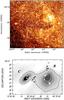 |
Fig. 1 Upper panel: DSS-R image of RCW 78. The cross marks the position of the WR star. The box encloses the two star-forming regions analyzed in this paper. Bottom panel: the two star-forming regions at 60 μm (IRAS data). The grayscale goes from 200 to 500 MJy sr-1, and the contour lines are from 240 to 300 MJy sr-1 in steps of 20 MJy sr-1, and from 350 to 500 MJy sr-1 in steps of 50 MJy sr-1. Regions B and C are indicated. The different symbols mark the location of candidate YSOs identified in Sect. 6: IRAS (star), CHII (triangle), 2MASS sources (crosses), and Spitzer sources (filled circles). |
Chu & Treffers (1981) found that the velocity of the ionized gas towards the brightest section of RCW 78 is in the range –53 km s-1 to –38 km s-1. Georgelin et al. (1988) identify Hα emission at –41.4 km s-1, compatible with Chu & Treffers’s results, and extended diffuse emission at –22 km s-1, most probably unrelated to RCW 78. Circular galactic rotation models (e.g., Brand & Blitz 1993) predict that gas having velocities between –53 km s-1 to –38 km s-1 lies at kinematical distances of 3.5–7.0 kpc. Taking into account the Ks-value for WR 55 from the 2MASS Survey (Cutri et al. 2003), an absolute magnitude MKs = −5.92 mag for WN7-9 (Crowther et al. 2006), and interstellar extinction values from Marshall et al. (2006), a distance in the range 4.5–5.0 kpc can be derived for the WR star, compatible with the kinematical distance of the ionized gas. Following CRMR09, we adopt a distance d = 5.0 ± 1.0 kpc.
A study of the molecular gas associated with the ring nebula RCW 78 was presented by CRMR09 with the aim of analyzing its distribution and investigating its energetics. The study was based on 12CO(1–0) and 12CO(2–1) observations of the brightest section of the nebula, carried out with the SEST telescope, and on complementary 12CO(1–0) data of a larger area obtained with the NANTEN telescope with an angular resolution of 27.
The authors reported the detection of molecular gas having velocities in the range –56 km s-1 to –33 km s-1 mainly associated with the western bright region of RCW 78, as well as an Hi envelope of the molecular gas, which is described in the same paper. The bulk of the molecular emission appears concentrated in two structures having velocities in the range –52.5 km s-1 to –43.5 km s-1 and from –43.5 km s-1 to –39.5 km s-1. Gas in the former velocity range is clearly linked to the western section of the nebula. According to CRMR09, material in the second velocity interval, which partially coincides with the dust lane present at RA(J2000) = –62° 22′, is also associated with RCW 78 based on the presence of Hα emission probably belonging to the nebula at these velocities (see Chu & Treffers 1981). This material may be connected to the receding part of an expanding shell linked to the nebula. Finally, material in the range –39 km s-1 to –33 km s-1 was only identified in a small region towards the brightest part of RCW 78, using SEST data.
Later on, Duronea et al. (2012; hereafter DAT12) performed a study of the molecular gas linked to the western and brightest section of the nebula. They based their analysis on NANTEN data having higher velocity resolution than CRMR09 and found molecular material linked to the western part of the nebula with velocities in the range –54 km s-1 to –46 km s-1 forming an expanding ring-like structure whose inner face is being ionized by the WR star.
A search for candidate young stellar objects (YSOs) performed by CRMR09 using the IRAS, Midcourse Space Experiment (MSX), and Spitzer point source catalogues, resulted in the detection of a number of candidates in two particular areas, suggesting the existence of two star forming regions (named regions B and C in CRMR09, and showed in the bottom panel of Fig. 1). These two areas coincide with molecular gas belonging to the neutral gas envelope detected around RCW 78, and so, the possibility that the expansion of the bubble has triggered star formation activity in the dense expanding envelope cannot be discarded.
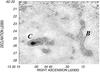 |
Fig. 2 870 μm continuum emission map obtained with LABOCA. The grayscale goes from –10 to 250 mJy beam-1. Contour levels correspond to 25, 50, 75, 100, 200, and 300 mJy beam-1. Regions B and C are indicated. |
The star forming regions are centered at RA, Dec(J2000) = (13h34m15s, –62°26′) (named region B in CRMR09) and at RA, Dec(J2000) = (13h35m05s, –62°25′30′′) (region C). Both regions are strong emitters at 60 μm, as can be seen in the bottom panel of Fig. 1. The O8Ib(f) star HD 117797 (RA, Dec(J2000) = (13h34m11.98s, –62° 25′ 1 8) (Walborn 1982), located at d ≃ 4 kpc, appears projected onto region B, which also coincides with the open cluster of A- and F-type stars C1331-622 located at 820 pc (Turner & Forbes 2005). Region C was previously catalogued as a star forming region by Avedisova (2002).
3. Observations
3.1. Continuum dust observations
3.1.1. LABOCA image
To accomplish this project we mapped the sub-millimeter emission at 870 μm (345 GHz) in an 8′ × 8′ field centered at RA, Dec(J2000) = (13h34m30s, –62°26′) with an angular resolution of 192 (HPBW), using the Large Apex BOlometer CAmera (LABOCA; Siringo et al. 2009) at 870 μm (345 GHz) operating with 295 pixels at the APEX 12-m sub-millimeter telescope.
The field was observed during 1.9 h in December 2009. The atmospheric opacity was measured every 1 h with skydips. Atmospheric conditions were very good (τzenith ≃ 0.25). The focus was optimized on Mars once during observations. The planet Mars was used as the primary calibrator, while the secondary calibrator was IRAS 13134-6264. The absolute calibration uncertainty is estimated to be 10%,
Data reduction was performed using CRUSH software3. The continuum emission map obtained with LABOCA is shown in Fig. 2. The noise level is in the range 10–15 mJy beam-1. Emission corresponding to regions B and C is indicated. Signal to noise for region B is S/N ≃= 10, with the higher value corresponding to the bright southern condensation. For region C, S/N = 40 at the peak position.
3.1.2. Herschel images
The far-IR images from Herschel Space Observatory were also used to trace cold dust emission. We used archival data at 70 and 160 μm taken with the Photodetector Array Camera and Spectrometer (PACS; Poglitsch et al. 2010) and data at 250, 350, and 500 μm obtained with the Spectral and Photometric Imaging REceiver (SPIRE; Griffin et al. 2010) observed by Herschel for the Hi-GAL key program (Hi-GAL: Herschel Infrared GALactic plane survey, Molinari et al. 2010, OBSIDs: 1342203055 and 1342203086). Both Herschel imaging cameras were used in parallel mode at 60 arsec/s satellite scanning speed with the purpose of obtaining simultaneous five-band images in a 2° × 2° field. The field we use is approximately centered at [l,b] = [–59°,0°].
Data reduction from archival data from the Level 2 stage for PACS and SPIRE maps was carried out using the Herschel interactive processing environment (HIPE v10, Ott & Herschel Science Ground Segment Consortium 2010) using the reduction scripts from standard processing. We made a non-oversampled mosaic for the PACS images and used a map merging script to merge two observations, one for each scan direction, performed in SPIRE parallel mode to produce a single map. To reconstruct the three SPIRE maps, we ran destriper gain corrections (HIPE v10, updated version by Schulz 2012) using the updated Level 1 SPIRE data.
To convert intensities from monochromatic values of point sources to monochromatic values of extended sources, assuming that an extended source has a spectral index alpha =4 (2 for the blackbody emission plus 2 for the opacity of the dust), the obtained fluxes of each source were multiplied by 0.98755, 0.98741, and 0.96787 for 250, 350, and 500 μm, respectively.
The angular resolutions at 70, 160, 250, 350, and 500 μm are 85, 135, 18′′, 25′′, and 36′′, respectively.
3.2. Molecular observations
The molecular gas distribution in the area of region B was investigated by performing 13CO(2–1) line observations (at 220.398677 GHz) of a region of 32 × 82 during December 2009, with the APEX telescope using the APEX-1 receiver, whose system temperature is Tsys = 150 K.
The half-power beamwidth of the telescope is 28 5. The data were acquired with a FFT spectrometer, consisting of 4096 channels, with a total bandwidth of 1000 km s-1 and a velocity resolution of 0.33 km s-1. The map was observed in the position switching mode. The off-source position free of CO emission is located at RA, Dec(J2000) = (13h33m10.3s, –62°2′41′′).
Calibration was performed using the planet Mars and X-TrA sources. Pointing was done twice during observations using X-TrA, o-Ceti and VY-CMa. The intensity calibration has an uncertainty of 10%.
The integration time per point was 14 s. The observed line intensities are expressed as main-beam brightness-temperatures Tmb, by dividing the antenna temperature  by the main-beam efficiency ηmb, equal to 0.75 for APEX-1.
The spectra were reduced using the Continuum and Line Analysis Single-dish Software (CLASS, of the Grenoble Image and Line Data Analysis Software working group)4. A linear baseline fitting was applied to the data. The typical rms noise temperature was 0.1 K (Tmb). The analysis was performed using the Astronomical Image Processing System (AIPS) and the CLASS software.
3.3. Complementary data
The millimeter and sub-millimeter data were complemented with infrared data retrieved from the MSX catalogue (Price et al. 2001), Spitzer images at 3.6, 4.5, 5.8, and 8.0 μm from the Galactic Legacy Infrared Mid-Plane Survey Extraordinaire (GLIMPSE; Benjamin et al. 2003), and images at 24 μm from the MIPS Inner Galactic Plane Survey (MIPSGAL; Carey et al. 2009).
Additional images of the Wide-field Infrared Survey Explorer (WISE; Wright et al. 2010) satellite at 3.4, 4.6, 12.0, and 22.0 μm with angular resolutions of 61, 64, 65, and 120 in the four bands were retrieved from IPAC5. In addition, an image at 1.4 GHz from the Southern Galactic Plane Survey (SGPS) published by DAT12 was used. The image has an angular resolution of 17 and an rms sensitivity below 1 mJy beam-1 (Haverkorn et al. 2006).
4. The distribution of the cold dust and molecular gas
4.1. Cold dust distribution
4.1.1. Region B
The upper panels of Fig. 3 display the emission at 870 μm in contours and grayscale for region B (left panel), and an overlay of the cold dust emission in contours and the IRAC emission at 8 μm (right panel). The continuum at 870 μm mainly originates in thermal emission from cold dust, while the emission at 8 μm is attributed to polycyclic aromatic hydrocarbons (PAHs) excited by UV photons.
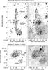 |
Fig. 3 Dust emission at 870 μm corresponding to regions B and C. Upper-left panel: dust emission for the filament and the southern clump (region B) in contours and grayscale. The image is smoothed to 25′′. The grayscale goes from 10 to 150 mJy beam-1, and the contours correspond to 20 to 100 mJy beam-1 in steps of 20 mJy beam-1. The position of candidate YSOs is indicated: 2MASS sources (crosses) and Spitzer sources (filled circles) (see Sect. 6). The position of the IRAS source is indicated by a star. Upper-right panel: overlay of the IRAC emission at 8 μm in grayscale and the 870 μm image in contours. The grayscale goes from 28 to 50 MJy sr-1. Bottom-left panel: dust emission for clumps 1 and 2 (region C) in contours and grayscale. The image is smoothed to 25′′. The grayscale goes from 10 to 500 mJy beam-1, and contours correspond to 40 to 200 mJy beam-1 in steps of 40 mJy beam-1, and 300 and 400 mJy beam-1. Bottom-right panel: overlay of the IRAC emission at 8 μm in grayscale and the 870 μm image in contours. The grayscale goes from 28 to 50 MJy sr-1. The symbols have the same meaning as in the upper panels. The position of the candidate CHII region is marked by a triangle. |
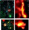 |
Fig. 4 Upper-left panel: composite image showing the IRAC emission of region B at 4.5 μm (in blue), 5.8 μm (in green), 24 μm (in red), and 870 μm (white contours). Contour levels correspond to 20, 40, 60, 80, and 120 mJy beam-1. Upper-right panel: composite image showing the Herschel emission of region B at 160 μm (in green) and 350 μm (in red), and the same contour levels as the image on the left. Bottom-left panel: composite image showing the IRAC emission of region C at 4.5 μm (in blue), 5.8 μm (in green), 24 μm (in red), and 870 μm (in white contours). Contour levels correspond to 20, 40, 80, 120, 160, 200, 300, and 400 mJy beam-1. Bottom-right panel: composite image showing the Herschel emission of region C at 160 μm (in green) and 350 μm (in blue), and the same contour levels as the image on the left. |
The emission at 870 μm consists of a filamentary structure elongated along the N-S direction (hereafter the filament), which ends to the south with a prominent bright condensation (hereafter the southern clump).
The southern clump, centered at RA, Dec(J2000) = (13h34m10.6s, –62°27′), is 25′′ in radius (0.60 pc at 5.0 kpc) and coincides with the brightest area at 8 μm. In Fig. 4 (left panel), we display the same LABOCA contours as Fig. 3 superimposed onto a composite image of the IRAC emissions at 4.5 μm (in red), 5.8 μm (in green), and 24 μm (in blue). The emission at 5.8 and 8 μm are coincident. A number of point-like sources can be identified within this clump at 4.5 μm, which are described in Sect. 6. Finally, emission linked to the clump is also detected at 24 μm, coincident with the sources at 4.5 μm. The right panel of Fig. 4 shows the emissions at 160 (in red) and 350 μm (in green). The image shows the excellent spatial correlation between the Herschel and LABOCA emissions. The clump is brighter at 160 μm than at 350 μm. The emissions at 250 and 350 μm are similar.
Candidate YSOs projected onto regions B and C.
The analysis of the IRAS point source catalogue, which has an angular resolution of 02 to 2′, allowed the identification of the source IRAS 13307-6211 (candidate to YSO/Class 0) as the counterpart at 60 and 100 μm of the southern clump. The fluxes and coordinates of this IRAS source are included in Table 1 (see below). The position of the IRAS source is indicated in Fig. 3 with a star.
The radio continuum emission distribution at 1.4 GHz shows an extended source (R ≈ 17) centered at RA, Dec(J2000) = (13h34m7.5s, –62°26′15′′) slightly to the north of the southern clump and to the west of the filament, named CF1 by DAT12. In spite of the low angular resolution of the radio continuum data (100′′) in comparison with the new IR data, the location of the source suggests that it may be related to the IR bubble described in Sect. 5, as stated by DAT12. However, the extension of the radio source towards the south suggests a contribution from the southern clump.
At 870 μm, the filament is about 45 in length (6.5 pc at 5 kpc), while its width, as meassured at 2σ level emission varies between 20′′ and 35′′ (0.5 and 0.8 pc, respectively), and is wider in the middle region. Several relatively faint maxima can be identified by eye in the filament. They are centered at RA, Dec(J2000) = (13h34m16s, –62° 26′ 40′′) (at 6σ level emission) and RA, Dec(J2000) = (13h34m16s, –62°25′15′′) (at 4σ level emission). These fainter emission regions do not have a clear counterpart at 8 μm. No emission is present at 4.5 μm, 5.8 μm, or at 24 μm (Fig. 4), suggesting that the filament lacks excitation sources. The strong emission region at 24 μm centered at RA, Dec(J2000) = (13h34m12s, –62°25′) is analyzed in Sect. 5 in connection with the small IR bubble.
The right panel of Fig. 4 shows that the emission at 160 μm detected by Herschel has a remarkable resemblance with the southern section of this filament (Dec(J2000) < –62°24′), while emission at 350 μm is detected all over the filament. At this last wavelength, the filament extends farther to the north than our LABOCA observations. There is a very good correlation with the LABOCA emission, although the Herschel emission is more extended in size.
At Dec(J2000) > –62°22′20′′, the emission at 8 μm is particularly low. Peretto & Fuller (2009) identified an infrared dark cloud (IRDC) at RA, Dec(J2000) = (13h34m16.04s, –62°22′52.2′′), less than 10′′ in size, coincident with a relatively bright section of the filament at 870 μm.
4.1.2. Region C
The emission at 870 μm corresponding to region C is displayed in the bottom panels of Fig. 3. The left panel shows this emission in contours and grayscale, while the right panel displays an overlay of the images at 870 and 8 μm. The image reveals two dust clumps. The brighter one is about 23 × 10 in size (3.3 × 1.5 pc at 5 kpc) (hereafter clump 1), while the smaller one is 10 × 07 in size (1.5 × 1.0 pc) (hereafter clump 2).
The brightest section of clump 1 coincides with strong emission at 8 μm centered at RA, Dec(J2000) = (13h35m4.1s, –62°25′45′′) (Fig. 3, right panel), with a bright source detected at 24 and 5.8 μm, and with a point-like source at 4.5 μm and 3.6 μm (Fig. 4, left panel). At 8 and 5.8 μm, the emission most probably originates in PAHs. Clearly, the emission at 24 μm suggests the presence of warm dust and an excitation source in the center of clump 1. The MSX source G307.9563+00.0163, classified as CHII (see Table 1) is projected onto the center of clump 1 (whose position is marked by a triangle).
Figure 4 (right panel) shows an overlay of the Herschel emission at 160 and 350 μm and the emission at 870 μm (in contours). The correlation between Herschel and LABOCA emissions is excellent.
Clump 1 coincides with a radio continuum source detected at 1.4 GHz, centered at RA, Dec(J2000) = (13h35m3s, –62°25′38′′) indicating the presence of ionized gas. The presence of radio continuum emission implies that a source of UV photons has created a compact HII region in the inner part of this clump.
A second and fainter source is detected at 8 μm at RA, Dec(J2000) = (13h35m0.7s, –62°25′385), close to the border of the 870 μm bright region. This source has counterparts at 3.6, 4.5, and 5.8 μm. Clump 2 is detected at both 160 and 350 μm. Instead, the emission is very faint in the mid IR at 5.8 and 8 μm. This small region displays weak radio continuum emission at 1.4 GHz.
4.2. The molecular gas
To illustrate the molecular gas components towards the filament and the southern clump, we show the 13CO(2–1) spectrum averaged in a region of 25 × 35 centered at RA, Dec(J2000) = (13h34m15s, –62°25′45′′) in Fig. 5. At least four velocity components are detected in the line of sight.
The bulk of the molecular emission peaks at ≃–53 km s-1, while fainter gas components are detected at ≃–63 and –37 km s-1. All velocities in this paper are referred to the local standard of rest (LSR). The molecular component at –37 km s-1 displays a double peak structure, while a small-scale structure is depicted by the component at –63 km s-1. Only a small amount of molecular gas at ≃–8 km s-1 can be identified. Finally, molecular emission was detected at ≃+20 km s-1. Molecular gas at –53 and –37 km s-1 was found to be linked to RCW 78 by CRMR09. As pointed out before, based on morphological arguments, molecular gas at –53 km s-1 is clearly linked to RCW 78, while the association of the component at –37 km s-1 might be uncertain according to DAT12.
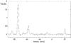 |
Fig. 5 13CO profile obtained by averaging the observed spectra in a region of 25 × 35 centered at RA, Dec(J2000) = (13h34m15s, –62°25′45′′). This region includes the filament and the southern clump. Intensity is expressed as main-beam brightness-temperature. |
To investigate the spatial distribution of the molecular gas in the line of sight to the filament and the southern clump, we analyzed the 13CO datacube. Figure 6 displays an overlay of the integrated emission ICO (= in selected velocity intervals and the LABOCA 870 μm emission for comparison. The emission in the range –64.8 km s-1 to –62.1 km s-1, which is displayed in panel a, is unconnected to the continuum emission detected at 870 μm.
Panel b shows gas with velocities in the range –55.1 km s-1 to –51.5 km s-1. An overlay of the molecular emission in contours and the dust emission obtained with LABOCA reveals the excellent correlation between the molecular gas at these velocities and the dust emission, with the brightest 13CO emission region coincident with the southern clump and its counterpart detected at 8 μm (panel d). The CO individual channel maps show that the peak 13CO emission coincident with the southern clump is detected in the range –55.1 km s-1 to –51.5 km s-1, while emission having velocities v ≥ − 52 km s-1 is detected north of –62°24′, coincident with the northern section of the filament. The 13CO spectrum (panel e) was obtained towards the center of the southern clump and shows that this velocity component is quite narrow (≃1.3 km s-1). The molecular filament, which coincides with the filament detected at 870 μm, can be identified in Fig. 5 in CRMR09 (see the panel for the velocity interval between –56.5 km s-1 to –53.5 km s-1) and in Fig. 4 in DAT12, where it is more apparent.
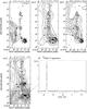 |
Fig. 6 Overlay of the integrated emission of the 13CO(2–1) line within selected velocity intervals (indicated in the upper part of each panel) in contours and the LABOCA image at 870 μm in grayscale. Panel a) contour lines are from 0.5 to 3.5 K km s-1 in steps of 0.5 K km s-1. Panel b) contours are from 1.5 to 12.0 K km s-1 in steps of 1.5 K km s-1, and 14.0 K km s-1. Panel c) contours are from 0.5 to 3.5 K km s-1 in steps of 0.5 K km s-1. Panel d) overlay of the 13CO contours of panel b) and the IRAC 8 μm emission (in grayscale). Panel e) 13CO spectrum towards the brightest region of the southern clump. |
The molecular gas showed in panel c (velocity interval from –38.9 km s-1 to –35.9 km s-1) partially coincides with the filament and may also be linked to the nebula. However, molecular gas at these velocities is absent in the profile obtained in the line of sight to the southern clump.
To sum up, our analysis confirms the presence of molecular gas in the range –55.1 km s-1 to –51.5 km s-1 clearly associated with region B, while the association of molecular gas in the interval –38.9 km s-1 to –35.9 km s-1 remains to be confirmed.
The molecular gas at v ≃ + 20 km s-1 is concentrated towards RA, Dec(J2000) = (13h34m12s, –62°25′) and will be discussed in Sect. 5.
The NANTEN data show that region C coincides with molecular gas in the range –43.5 km s-1 to –39.5 km s-1 (see CRMR09 and DAT12). The connection of this region to the nebula is an open question since it is not yet clear if material at these velocities is linked to the nebula.
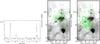 |
Fig. 7 Left panel: 13CO spectrum at the center of the molecular gas at +20 km s-1 (RA, Dec(J2000) = (13h34m17.2s, –62°25′)). Intensity is expressed as main-beam brightness temperatures. Middle panel: overlay of the integrated emission of the 13CO(2–1) line within the velocity interval from +19.5 to +21.5 km s-1 and the emission at 8 μm from IRAC. Contours are 0.5 to 4.0 K km s-1 in steps of 0.6 K km s-1. Right panel: overlay of the integrated emission in the velocity interval from –37.7 to –37.0 km s-1 and the emission at 8 μm. Contours are 0.39, 0.46, 1.3, 2.0, and 2.6 K km s-1. |
5. The small IR bubble
An inspection of the IRAC image at 8 μm reveals a striking ring of about 16′′ in radius centered at RA, Dec(J2000) = (13h34m12s, –62°25′). The structure resembles some of the IR dust bubbles identified by Churchwell et al. (2006) at 8 μm and Mizuno et al. (2010) at 24 μm. The WISE images at 12 and 22 μm show an extended source coincident with the IR bubble. A close inspection of the brightest part of this source reveals a faint ring coincident with the bubble, which is also identified at 24 μm (DAT12) and in the Herschel image at 70 μm. The image at 12 μm includes the emission from prominent PAH features. Emission at 22 μm (WISE) and 24 μm (MIPSGAL) indicate the presence of warm dust (Wright et al. 2010). The MSX point source G307.8603+00.0439, listed in Table 1 of CRMR09 as a candidate CHII region, is resolved as the IR bubble in the IRAC 8 μm image. We note that the angular resolution of the IRAC image is 9 times better than that of the MSX image.
In Fig. 7 we display a 13CO spectrum obtained slightly to the east of the IR bubble at RA, Dec(J2000) = (13h34m17.2s, –62°25′), showing three intense velocity components. The emission near –53 km s-1 corresponds to the molecular gas linked to the filament and is unconnected to the IR bubble. The emission distribution at +20 and –37 km s-1 is displayed in the center and bottom panels of the figure in contours, with the emission at 8 μm in grayscale for comparison.
The bulk of the molecular emission in the range from +19.5 km s-1 to +21.5 km s-1 appears projected onto the small IR bubble, while weak emission is also present in the line of sight to the southern clump. The circular galactic rotation model by Brand & Blitz (1993) predicts that gas at these velocities should be located outside the solar circle at distances of ≃11 kpc. An analysis of the spatial distribution of the Hi gas emission at positive velocities using the Southern Galactic Plane Survey (McClure-Griffiths et al. 2005) and that of the molecular gas based on the 12CO(1–0) line observations of the NANTEN telescope, reveals the existence of neutral atomic and molecular gas at large scale in the line of sight at v ≃ + 20 km s-1 (CRMR09).
The bottom panel exhibits the emission of the molecular gas having velocities in the interval –37.7 km s-1 to –37.0 km s-1. The image shows that the 13CO contours delineate the eastern borders of the IR bubble, suggesting that the nebula is interacting with the molecular material. The existence of molecular emission partially surrounding the IR bubble is compatible with the presence of PAHs emission, which suggests that a photodissociation region (PDR) has developed in the borders of the molecular cloud. All of which, along with the existence of warm dust, suggests that an excitation source should be powering the bubble.
The star HD 117797 (O8Ib[f], Maíz-Apellániz et al. 2004) appears projected in the center of the IR bubble. Taking into account an absolute magnitude Mv = −6.2 mag (Lang 1991) and an absorption Av = 2.4 mag derived from photometric data in the Galactic O Stars Catalog (GOS, Maíz-Apellániz et al. 2004), a distance of 4.0 kpc can be estimated. Since HD 117797 is the only massive star catalogued in this area, as a working hypothesis we propose that HD 117797 is the exciting star of the IR bubble, placing it at 4 kpc. We believe that this star has created the bubble through the action of its stellar wind and UV photons.
The IR bubble resembles the rings identified by Mizuno et al. (2010) at 24 μm, and share some characteristics with them, in particular its size and its correlation with emission at 8 μm. According to these authors, a large fraction of these rings are planetary nebulae. However, the presence of the O8Ib(f) star in the center of the IR structure puts aside a planetary nebula interpretation.
The MSX source G307.8561+00.0463, at RA, Dec(J2000) = (13h34m10.2s, –62°25′), classified as massive young stellar object (MYSO) following Lumsden et al. 2002 (see CRMR09) appears projected onto the ring detected at 8 μm. This source has a counterpart at 24 μm. Since this source probably shows emission from warm dust in the bubble, it is not included in Table 1. The MSX source G307.8620+00.0399 listed in Table 1 from CRMR09 turned out to be a false detection.
Higher sensitivity and angular resolution molecular and radio continuum data are necessary to properly investigate if molecular gas is linked to the nebula and to reveal if ionized gas is present.
6. Identification of YSOs
As pointed out in Sect. 1, a search for candidate YSOs in the environs of regions B and C was performed by CRMR09 using the IRAS, MSX, and Spitzer point source catalogues. The results of the search in the IRAS and MSX catalogues are given in Table 1.
To search for YSO candidates with better spatial resolution than IRAS and MSX, we used 2MASS sources having good photometric quality (S/N > 10), in the (H − KS, J − H) diagram in a region of 8′ × 8′ centered at RA, Dec(J2000) = (13h34m33.75s, –62°25′34′′). We found 32 candidate YSOs. Nine out of 32 candidate YSOs spatially coincide with regions emitting at 870 μm. Their coordinates, names, J,H, and KS magnitudes, and MIR-information from Spitzer appear in the middle part of Table 1. Only three sources have been detected in all IRAC bands (5, 7, and 11). The upper panel of Fig. 10 shows the 2MASS CC diagram with the candidate YSOs represented by blue squares. In spite of the small infrared excess of the sources, their location in the diagram suggests that they are low-mass young stellar objects.
We have performed a new search for candidate YSOs using the Spitzer database taking into account sources detected in the four IRAC bands following Allen et al. (2004) and Hartmann et al. (2005), which allows the IR sources to be discriminated according to a class scheme: Class I are protostars surrounded by dusty infalling envelopes; Class II are objects whose emission is dominated by accretion disks; and Class III are sources with an optically thin or no disk. An analysis of the nature of the Spitzer sources in the same region defined for the 2MASS sources revealed that 29 of the 944 IR sources can be classified as candidate YSOs.
The bottom panel of Fig. 10 shows the position of the 29 Spitzer sources in the diagram [3.6]–[4.5] vs. [5.8]–[8.0]. These 29 sources are indicated by gray crosses. We note that because of the revision and reclassification of the candidates listed in CRMR09, the candidate YSOs identified from the Spitzer point source catalog listed in Table 1 of this paper differs from the ones published in CRMR09, which were mistakenly identified.
Twelve out of these 29 sources coincide with regions emitting at 870 μm. Their IR photometry information is summarized in the bottom part of Table 1. Most of these sources have a counterpart in the 2MASS database. Four out of these 12 sources are represented by open triangles superimpossed onto the crosses in the bottom panel of Fig. 10. They correspond to candidate YSOs without a 2MASS counterpart (12, 13, 17, and 22), while filled triangles indicate sources with only KS, and H and KS magnitudes (14 and 20). All but one (22) lie in the overlapping region between low-luminosity Class I sources and Class II sources (12, 13, 17, and 20). The other six sources (indicated by asterisks) lie in the limit region between Class II and III sources in the [3.6]–[4.5] vs. [5.8]–[8.0] diagram, which is highly contaminated by evolved stars. Source 15 has the most highly reddened [5.8]–[8] color in the sample.
The 2MASS CC diagram of the upper panel of Fig. 10 indicates that Spitzer sources 16, 18, 21, and 23 (represented by red asterisks) are candidates to giant stars. The other two Spitzer sources with 2MASS counterparts (15 and 19) are situated in the main sequence star domain (represented by green filled squares in the upper panel). We note that reddened main sequence stars and highly obscured YSOs can coincide in the locus of the 2MASS diagram (Robitaille et al. 2006, see Sect. 3.4.2.1). Spitzer colors corresponding to source 15 are typical of photodissociation regions (PDR), suggesting its association with molecular gas.
Class III lie in the region occupied by foreground and background stars, as do 2MASS candidate YSOs with Spitzer colors. They are indicated by open squares in the right panel of Fig. 10. Sources without measurements at 5.8 and 8 μm are not included.
Finally, a close inspection of the the IRAC images at 3.6 and 4.5 μm reveals a cluster of IR sources coincident with the southern clump. Figure 8 shows a composite image with the emissions at 3.6 μm in red, at 4.5 μm in green, and at 5.8 μm in blue, with the sources in the cluster. These sources have counterparts in the 2MASS Survey and are listed in Table 2, which shows their positions, names, and 2MASS fluxes. The analysis of the 2MASS data allows the identification of one YSO (source 3 en Table 1, which is also source 3 in Table 2), one giant star, and some main sequence stars. On the other hand, the Spitzer catalog lists 41 sources projected onto the southern clump. Only five of them have measurements in the four bands and cannot be classified as YSOs. Measured fluxes with HIPE at 3.6 and 4.5 μm for the 2MASS sources are indicated in Cols. 8 and 9 in Table 2. Sources 3 and 8 in Table 2 coincide with point-like emission at 24 μm, with fluxes of 340 and 48 mJy, respectively. These measurements are compatible with an YSO nature of source 3.
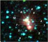 |
Fig. 8 Composite image of the cluster within the southern clump showing the IRAC emission at 3.6 (in blue), 4.5 (in green), and 5.8 μm (in red). North is up and east to the left. The size of the image is 82′′ in RA and 75′′ in Dec Data for the different sources are given in Table 2. |
6.1. Characteristics of the YSOs based on their SEDs
To complete the photometric analysis, we inspected the spectral energy distribution (SED) of the 2MASS and Spitzer sources. We used the online6 tool developed by Robitaille et al. (2007), which can help to discriminate between evolved stars and reliable candidate YSOs. This tool fits radiation transfer models to observational data according to a χ2 minimization algorithm. We chose the models that met the condition  (1)where
  is the minimum value of the χ2 among all models, and n is the number of input data fluxes.
Cluster of IR sources within the southern clump.
Main parameters of the SEDs.
To perform the fittings we used the photometric data listed in Table 1 along with visual extinction values in the range 5–12 mag (derived from the 2MASS CC diagram), and distances in the range 4.0–6.0 kpc. No observational data longwards of 10 μm are available for these sources (e.g., MSX, Herschel), except for sources 7, 19, and 22. The available optical flux for source 7 was obtained by averaging B,V, and R magnitudes from the USNO B-1.0 catalog (Zacharias et al. 2004) and the NOMAD catalog (Monet et al. 2003).
The results of the analysis applied to the candidate YSOs are summarized in Table 3. Column 1 gives the number of the source according to Table 1; Col. 2, the value of χ2 for the best fitting, χ2/n; Col. 3, the number of input data fluxes used in the fitting, n; Col. 4, the number of models that satisfies Eq. (1), N; Col. 5, the mass of the central source, M★; Col. 6, the mass of the disk, Mdisk; Col. 7, the envelope and ambient density mass, Menv; Col. 8, the infall rate, Ṁenv; Col. 9 gives the total luminosity, LTOT; Cols. 10 and 11, the classification according to Allen et al. (2004) and Robitaille et al. (2007), respectively; and Col. 12, the age of the central object.
The information in Col. 10 is an estimate of the evolutionary stage of the objects based on their physical properties. Based on ratios of these parameters, the sources can be separated into three categories, from objects with significant infalling envelopes and possible disks (Stage 0/I) to objects with optically thin disks (Stage III). The stages are defined by these cutouts: sources which have Ṁenv/M★ > 10-6 yr-1 indicate Stage 0/I, Ṁenv/M★ < 10-6 yr-1 and Mdisk/M★ > 10-6 correspond to Stage II, and, finally, Ṁenv/M★ < 10-6 yr-1 and Mdisk/M★ < 10-6 for Stage III.
Fittings of sources 14 and 16 are consistent with Stage I. They have Ṁenv > 0 and the largest mass envelopes, indicating that they could be young objects inmersed in prominent envelopes.
Candidate main sequence stars are fitted by Stage III models. For the case of source 15, the models suggest that the object is an intermediate mass star (3–5 M⊙). However, its position in the 2MASS CC diagram casts doubts on this interpretation. The SED of source 19 corresponds to a massive star (8 M⊙) with an optically thick disk and an infalling envelope with undetected accretion.
The results of the fittings should be taken with caution, since the fitting tool has some limitations. As demonstrated by Deharveng et al. (2012) and Offner et al. (2012; see also Robitaille 2008), the inferred disk and envelope properties and the evolutionary status vary with the viewing angle, the gas morphology, the dust characteristics, and the multiplicity of the sources.
Finally, the fitting of a Kurucz photospheric model gives an additional way to evaluate the nature of sources with NIR colors corresponding to giants in the (H − KS, J − H) diagram, which lie at the limit of the Class II–III region. The SED of sources 18, 21, and 23 can be fitted by a photospheric model with an effective temperature of ≈5000 K, indicating that they are evolved stars. Consequently, they can be discarded as candidate YSOs and are not included in Table 3.
The whole sample shows colors [3.6]–[4.5] < 1.1, in agreement with moderate or low values of Ṁenv. This behavior is related to the accretion rate since the redder the source in [3.6]–[4.5] color, the higher the Ṁenv (Allen et al. 2004).
We applied the SED analysis to the 2MASS candidate YSOs. We were able to discern the evolutionary stage of source 7 only, for which we used fluxes from USNO, NOMAD, 2MASS, Spitzer, and WISE databases. The fitting suggests that this would be the oldest source with an age of 7 × 10⁶ yr. The derived SED is shown in Fig. 9.
To sum up, we have not found massive objects in our sample. Source 16 is consistent with Stages I/II, while 7 and 15 seem to be objects in Stage III with ages larger than 106 yrs.
6.2. Spatial distribution
The position of the YSOs listed in Table 1 is indicated in Figs. 1 and 3. The star and triangle mark the location of the IRAS source and the compact HII region (CHII), respectively. The IRAS and MSX sources cannot be considered point-like sources. Circles and crosses correspond to Spitzer and 2MASS point sources, respectively.
The IR cluster, which includes source 3 from Table 1, coincides with the southern clump, which is clearly a star forming region.
A number of sources appear projected onto the filament. Among these sources, source 15 may show the presence of molecular gas. The spatial coincidence of this source with both gas emission at –37 km s-1 and +20 km s-1 precludes the identification of the associated gas, if any. Finally, Spitzer sources 13 and 14 and the 2MASS sources 6, 7 and 8 are projected onto the northern extreme of the filament.
Source 8 is placed near the infrared dark cloud IRDC 307.873+0.079 (Wilcock et al. 2012). This IRDC has a major axis of 9′′ in size and was detected at 250 μm. Wilcock et al. (2012) suggested that it is an HII region starting to form; however, no counterparts at wavelengths larger than 4.5 μm are detected.
The presence of a candidate CHII region and emission at 24 μm in clump 1 suggests that there was star formation activity.
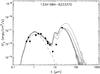 |
Fig. 9 SED of the 2MASS source 7. Input data are indicated by filled circles. The triangle indicates an upper limit at 22 μm (from WISE). The black line corresponds to the best fitting. The fittings which obey Eq. (1) appear indicated by gray lines. The dashed lines show the emission of the stellar photosphere including foreground interstellar extinction. Fittings for source 7 indicates a Stage III object, being the oldest source in the sample. |
7. Gas and dust parameters
7.1. Masses from submillimeter data
With the aim of estimating cold dust masses, it is necessary to subtract the contribution of different gas phases from the emission at 870 μm. Two processes may contribute to the emission at this wavelength in addition to the thermal emission from cold dust: molecular emission from the CO(3–2) line and free-free emission from ionized gas. The continuum emission contribution at 345 GHz due to ionized gas was estimated from the radio continuum image at 5 GHz published by CRMR09, considering that the radio emission at 5 GHz is thermal, using the expression S345 = (345/5)-0.1S5 GHz. The contribution from the CO(3–2) line was roughly estimated from our CO data taking into account a ratio C0(3–2)/CO(2–1) = 1.0–1.6 (Myers et al. 1983) and an intensity ratio I(12CO/13CO) = 4–5 for our Galaxy. The total contribution of both mechanisms is about 10% for the southern clump and the filament and less than 5% for clumps 1 and 2, and consequently, within the flux uncertainties.
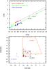 |
Fig. 10 Upper panel: [H − Ks, J − H] diagram of the 2MASS and Spitzer candidate YSOs. 2MASS candidate YSOs are indicated by blue squares. 2MASS colors of Spitzer candidates are indicated by asterisks and filled green squares. They are located in the giant and main sequence regions of the diagram. The dashed lines show the reddening vectors corresponding to M0 III and B2 V stars. The crosses are placed at intervals of five magnitudes of visual extinction. Bottom panel: location of candidate YSOs from the Spitzer database. Crosses represent the 29 sources which lie in Class I and II regions. Triangles, asterisks, and filled squares correspond to sources projected onto the filament, the southern clump and clumps 1 and 2, respectively. Open and filled triangles represent candidate YSOs that do not have a 2MASS counterpart and those that have been detected in one or two filters only, respectively. Spitzer sources with 2MASS colors are indicated by asterisks and filled rectangles. They occupy the main sequence and giant regions in the upper panel. 2MASS sources with Spitzer colors are indicated by optn squares. They lie in the Class III region where main sequence, giants, and pre-main sequence stars overlap. |
Fluxes from Herschel images.
Considering that the emission detected at 870 μm originates in thermal dust emission, an estimate of the dust mass can be derived. Assuming that the dust emission is optically thin, and following Deharveng et al. (2009), the dust mass can be obtained as  (2)In this expression, S870 is the measured flux density integrated over the area described by the 2σ level of the LABOCA map of the source, d is the distance to the source, κ870 is the dust opacity per unit mass at 870 μm, and B870(ν,Tdust) is the Planck function for a temperature Tdust. We adopt κ870 = 1.38 cm2 g-1 (Miettinen 2012).
Dust temperatures Tdust were obtained from the Herschel and LABOCA images. Fluxes for the southern clump at 70, 160, 250, 350, and 500 μm were obtained with HIPE using annular aperture sky photometry. To measure the flux, the filament was divided into five circular sections. For each area, we measured the average surface brightness. Flux uncertainty comes from uncertainties in surface brightness and flux calibration. The results are summarized in Table 4. Columns 2–6 list the derived fluxes. Total fluxes are listed in this table for the filament.
In Fig. 11 we display the SEDs and the best fitting obtained for the southern clump, the filament, and the brightest section of clump 1 after convolving the Herschel and LABOCA images to the angular resolution of the image at 500 μm and taking into account the same apertures for all the wavelengths. Background emission was subtracted from the Herschel images. The SEDs for the southern clump and clump 1 include the flux obtained at 870 μm. Derived dust temperature are listed in Col. 7 of Table 4. They are compatible with Tdust = 20–30 K, generally assumed for protostellar condensations (see Motte et al. 2003; Deharveng et al. 2009; Johnstone & Bally 2006; Fontani et al. 2004).
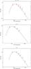 |
Fig. 11 SEDs for the southern clump (upper panel), the filament (middle panel), and clump 1 (bottom panel) obtained using data in the far IR. |
Table 5 lists the parameters derived for the southern clump, the filament, and clumps 1 and 2 separately from the molecular and LABOCA data. In the table we include the size of the source, the flux density, and dust and total masses. Fluxes included in this table correspond to the whole extension of each source. The dust mass Mdust for clump 2 was obtained using Tdust = 20–30 K, while masses for the other structures were estimated using the dust temperature obtained from the SEDs. The total mass Mtot was estimated adopting a typical gas-to-dust mass of 100.
7.2. Parameters of the molecular gas
The molecular mass associated with the southern clump and the filament can be evaluated from the 13CO line using local thermodynamic equilibrium (LTE).
Assuming LTE, the H2 column density, N(H2), can be estimated from the 13CO(2–1) line data following the equations of Rohlfs & Wilson (2004)![Mathematical equation: \begin{eqnarray} N_{\rm tot}(^{13}{\rm CO}) = 1.5 \times 10^{14}\ \frac{{\rm e}^{\left[\frac{T_0 (\nu_{10})}{T_{\rm exc}}\right] }\ \ \ T_{\rm exc} \int \tau^{13}\ \ {\rm d}v} {1 - {\rm e}^{\left[\frac{-T_0 (\nu_{21})}{T_{\rm exc}} \right]} } \quad \textrm{ (cm}^{-2}), \label{n13co} \end{eqnarray}](/articles/aa/full_html/2014/02/aa20990-12/aa20990-12-eq114.png) (3)where τ13 is the opacity of the 13CO(2–1) line, ν10 the frequency of the 13CO (1–0) line (110.201 GHz), T0(ν21) = hν21/k, and ν21 the frequency of the 13CO(2–1) line. Assuming that τ13 ≪ 1 , the integral of Eq. (3) can be aproximated by
(3)where τ13 is the opacity of the 13CO(2–1) line, ν10 the frequency of the 13CO (1–0) line (110.201 GHz), T0(ν21) = hν21/k, and ν21 the frequency of the 13CO(2–1) line. Assuming that τ13 ≪ 1 , the integral of Eq. (3) can be aproximated by  (4)Then, the molecular mass is calculated using
  (5)where msun is the solar mass (~2 × 1033 g), μ is the mean molecular weight (assumed to be equal to 2.8 after allowance of a relative helium abundance of 25% by mass; Yamaguchi et al. 1999), mH is the hydrogen atom mass (~1.67 × 10⁻²⁴ g), Ω is the solid angle subtended by the CO clump in sr, d is the assumed distance expressed in cm, and N(H2) is the H2 column density obtained using the canonical abundance N(H2)/N(13CO) = 5 × 10⁵ (Dickman 1978). Assuming that τ13 ≪ 1 and τ12 ≫ 1, the opacity of the 13CO(J = 2 → 1) line can be derived using
 ![Mathematical equation: \begin{eqnarray} \tau^{13} = -{\rm ln}\left[1-\frac{T_{\rm b}(^{13}{\rm CO})}{T_0^{13}} \left[\left({\rm e}^{\frac{T_0^{13}} {T_{\rm exc}}}-1 \right)^{-1}-f(T_{\rm bg})\right]^{-1}\right], \label{tau13co} \end{eqnarray}](/articles/aa/full_html/2014/02/aa20990-12/aa20990-12-eq135.png) (6)where
(6)where  /k,
/k, ![Mathematical equation: \hbox{$f(T) = \left[ {\rm e}^{T_0^{13} / T} -1 \right]^{-1}$}](/articles/aa/full_html/2014/02/aa20990-12/aa20990-12-eq138.png) , and Tb = 2.7 K. Since the optically thick 12CO(2–1) line was not observed, Texc could not be derived directly from our data. Hence, we have adopted Texc = 20–40 K for the southern clump in agreement with values adopted by Brand et al. (2001), Deharveng et al. (2008b), and Pomarès et al. (2009). Similar values were adopted for the filament. It is worth pointing out that uncertainties of 50% in the values of Texc yields to total M(H2)-uncertainties of up to 25%.
, and Tb = 2.7 K. Since the optically thick 12CO(2–1) line was not observed, Texc could not be derived directly from our data. Hence, we have adopted Texc = 20–40 K for the southern clump in agreement with values adopted by Brand et al. (2001), Deharveng et al. (2008b), and Pomarès et al. (2009). Similar values were adopted for the filament. It is worth pointing out that uncertainties of 50% in the values of Texc yields to total M(H2)-uncertainties of up to 25%.
The results for the southern clump and the filament are indicated in Table 5, which lists the integrated emission of 13CO within the velocity interval from –55.1 km s-1 to –51.5 km s-1, the optical depth, the solid angle and the effective radius where the molecular emission is present, the column density of 13CO and molecular hydrogen, the molecular mass, and the ambient density. Errors in masses due to distance uncertainties (20%) are about 40%. The ambient density of the southern clump was estimated by distributing the total mass in a sphere of 1.35 pc in radius, while for the filament, we distributed the molecular mass in a region of 8 pc in lengh, 2.7 pc in width, and 2.7 pc along the line of sight.
We note that in the southern clump, the molecular gas was detected in a larger area than the cold dust. The difference in the emission areas may be due to the presence of emission below the 2σ limit in the LABOCA data and/or a higher gas-to-dust ratio in the outer areas of the southern clump. To compare the masses derived from the dust continuum Mtot and from the molecular line, we need to integrate the emissions within the same area. Consequently, we evaluated the molecular mass using LTE in the same area where the dust continuum emission was detected (equal to the area of a circle of R = 0.6 pc). We obtained a total mass  .
.
Dust and molecular gas parameters.
We can obtain the virialized mass for this clump and compare it with Mtot and  . Assuming a spherically symmetric cloud with a constant density distribution, the virial mass can be determined from (MacLaren et al. 1988)
 ![Mathematical equation: \begin{eqnarray} \label{eq:mvir} M_{\rm vir} = 210~R (\Delta v_{\rm cld})^2~[M_\odot], \end{eqnarray}](/articles/aa/full_html/2014/02/aa20990-12/aa20990-12-eq162.png) (7)where R = 0.6 pc, and Δ vcld = 1.5 km s-1 is its velocity dispersion in km s-1, which is defined as the FWHM line width of the composite profile derived by using a single Gaussian fitting. The composite profile is obtained by averaging the spectra within R. The resulting virial mass is Mvir = 280 M0. The agreement between the masses derived using the LTE model and the virial theorem is within a factor of 3, while the agreement of the molecular and virial masses with the mass derived from the dust continuum emission is within a factor of 2–6.
(7)where R = 0.6 pc, and Δ vcld = 1.5 km s-1 is its velocity dispersion in km s-1, which is defined as the FWHM line width of the composite profile derived by using a single Gaussian fitting. The composite profile is obtained by averaging the spectra within R. The resulting virial mass is Mvir = 280 M0. The agreement between the masses derived using the LTE model and the virial theorem is within a factor of 3, while the agreement of the molecular and virial masses with the mass derived from the dust continuum emission is within a factor of 2–6.
The mass of the southern clump is similar to masses derived for other star forming regions (see, e.g., Mookerjea et al. 2004, Deharveng et al. 2009; Sánchez-Monge et al. 2008).
8. Conclusions
We have investigated the presence of molecular clouds and dust clumps linked to the star forming regions B and C previously identified in CRMR09, by performing APEX observations of the continuum 870 μm dust and 13CO(2–1) molecular line emissions, and by analyzing IRAC and Herschel images in the near- and far-IR.
The continuum sub-millimeter observations towards region B allowed the identification of a filament elongated in the N-S direction, ending in a bright condensation (that we have named the southern clump). This southern clump, which can be identified with IRAS 13307-6211, is 25′′ in radius (or 0.6 pc at 5 kpc), and coincides with bright patches of emission at 5.8 and 8 μm, and in the Herschel images at 70, 160, 250, 350, and 500 μm. The presence of radio continuum emission probably linked to the clump and emission at 24 μm suggests the existence of excitation sources inside. The identification of a cluster or IR sources detected in the 2MASS and IRAC images, which includes young stellar objects, showed that star formation is active in this region.
The filament can also identified in the Herschel images. Instead, it is not detected in the near IR. A number of candidate YSOs are projected onto the filament.
The distribution of the 13CO emission revealed that molecular gas with velocities in the interval –55.1 km s-1 to –51.5 km s-1 is the molecular counterpart of the dust filament and the southern clump. The velocity of the molecular gas is compatible with its location in the expanding envelope of RCW 78.
Towards region C, two cold dust clumps were identified both in the LABOCA and Herschel images. The brightest section of the larger clump coincides with emission at 5.8 μm and 8 μm. The presence of radio continuum emission at 1.4 GHz is indicative of ionized gas and a source of UV photons inside. Indeed, an MSX source classified as candidate CHII region reinforces the idea that moderate star formation has occured recently. It is not clear at this time if this region is linked to RCW 78.
We estimated total masses for the dust condensations from the emission at 870 μm and from the molecular line using LTE and the virial theorem. Masses for the filament and the southern clump obtained through different methods agree within a factor of 2–6. Dust temperatures derived from far-IR data for the dust clumps and the filament are about 30 K, compatible with those of protostellar condensations.
The 8 μm IRAC image revealed the existence of an infrared dust bubble of 16′′ in radius centered at RA, Dec(J2000) = (13h34m12s, –62°25′) with a clear counterpart at 24 μm, suggesting the existence of warm dust in the ring. The bubble is probably linked to the O-type star HD 117797 located at 4 kpc and may be interacting with the molecular gas, although molecular gas linked to it cannot be clearly identified from the present observations. The presence of the PAH emission seen at 8 μm and of warm dust is compatible with an O-type star as the excitation source powering the bubble.
APEX is a collaboration between the Max-Planck-Institut fur Radioastronomie, the European Southern Observatory, and the Onsala Space Observatory.
Herschel is an ESA space observatory with science instruments provided by European-led Principal Investigator consortia and with important participation from NASA.
Acknowledgments
C.E.C. acknowledges the kind hospitality of Dr. M. Rubio and her family during her stays in Santiago, Chile. We acknowledge the many constructive comments and suggestions of the referee, which helped to improve this paper. This project was partially financed by CONICET of Argentina under project PIP 02488 and UNLP under project 11/G120. M.R. is supported by CONICYT of Chile through grant No. 1080335. V.F. would like to thank Ivan Valtchanov for his support and valuable assistance in Herschel data processing. This research has made use of the NASA/IPAC Infrared Science Archive, which is operated by the Jet Propulsion Laboratory, California Institute of Technology, under contract with the National Aeronautics and Space Administration. This work is based [in part] on observations made with the Spitzer Space Telescope, which is operated by the Jet Propulsion Laboratory, California Institute of Technology under a contract with NASA. This publication makes use of data products from the Two Micron All Sky Survey, which is a joint project of the University of Massachusetts and the Infrared Processing and Analysis Center/California Institute of Technology, funded by the National Aeronautics and Space Administration and the National Science Foundation. The MSX mission is sponsored by the Ballistic Missile Defense Organization (BMDO).
References
- Allen, L. E., Calvet, N., D’Alessio, P., et al. 2004, ApJS, 154, 363 [NASA ADS] [CrossRef] [Google Scholar]
- Avedisova, V. S. 2002, Astron. Rep., 46, 193 [NASA ADS] [CrossRef] [Google Scholar]
- Benjamin, R. A., Churchwell, E., Babler, B. L., et al. 2003, PASP, 115, 953 [NASA ADS] [CrossRef] [Google Scholar]
- Brand, J., & Blitz, L. 1993, A&A, 275, 67 [NASA ADS] [Google Scholar]
- Brand, J., Cesaroni, R., Palla, F., & Molinari, S. 2001, A&A, 370, 230 [NASA ADS] [CrossRef] [EDP Sciences] [Google Scholar]
- Cappa, C. E., Rubio, M., Martín, M. C., & Romero, G. A. 2009, A&A, 508, 759 (CRMR09) [NASA ADS] [CrossRef] [EDP Sciences] [Google Scholar]
- Carey, S. J., Noriega-Crespo, A., Mizuno, D. R., et al. 2009, PASP, 121, 76 [NASA ADS] [CrossRef] [Google Scholar]
- Chu, Y.-H., & Treffers, R. R. 1981, ApJ, 250, 615 [NASA ADS] [CrossRef] [Google Scholar]
- Crowther, P. A., Hadfield, L. J., Clark, J. S., Negueruela, I., & Vacca, W. D. 2006, MNRAS, 372, 1407 [NASA ADS] [CrossRef] [Google Scholar]
- Cutri, R. M., Skrutskie, M. F., van Dyk, S., et al. 2003, 2MASS All Sky Catalog of point sources [Google Scholar]
- Deharveng, L., Lefloch, B., Kurtz, S., et al. 2008a, A&A, 482, 585 [NASA ADS] [CrossRef] [EDP Sciences] [Google Scholar]
- Deharveng, L., Lefloch, B., Kurtz, S., et al. 2008b, A&A, 482, 585 [NASA ADS] [CrossRef] [EDP Sciences] [Google Scholar]
- Deharveng, L., Zavagno, A., Schuller, F., et al. 2009, A&A, 496, 177 [NASA ADS] [CrossRef] [EDP Sciences] [Google Scholar]
- Deharveng, L., Schuller, F., Anderson, L. D., et al. 2010, A&A, 523, A6 [NASA ADS] [CrossRef] [EDP Sciences] [Google Scholar]
- Deharveng, L., Zavagno, A., Anderson, L. D., et al. 2012, A&A, 546, A74 [NASA ADS] [CrossRef] [EDP Sciences] [Google Scholar]
- Dickman, R. L. 1978, ApJS, 37, 407 [NASA ADS] [CrossRef] [Google Scholar]
- Duronea, N. U., Arnal, E. M., & Testori, J. C. 2012, A&A, 540, A121 (DAT12) [NASA ADS] [CrossRef] [EDP Sciences] [Google Scholar]
- Elmegreen, B. G., & Lada, C. J. 1977, ApJ, 214, 725 [NASA ADS] [CrossRef] [Google Scholar]
- Fontani, F., Cesaroni, R., Testi, L., et al. 2004, A&A, 424, 179 [NASA ADS] [CrossRef] [EDP Sciences] [Google Scholar]
- Georgelin, Y. M., Boulesteix, J., Georgelin, Y. P., Le Coarer, E., & Marcelin, M. 1988, A&A, 205, 95 [NASA ADS] [Google Scholar]
- Griffin, M. J., Abergel, A., Abreu, A., et al. 2010, A&A, 518, L3 [Google Scholar]
- Hartmann, L., Megeath, S. T., Allen, L., et al. 2005, ApJ, 629, 881 [NASA ADS] [CrossRef] [Google Scholar]
- Haverkorn, M., Gaensler, B. M., McClure-Griffiths, N. M., Dickey, J. M., & Green, A. J. 2006, ApJS, 167, 230 [CrossRef] [Google Scholar]
- Johnstone, D., & Bally, J. 2006, ApJ, 653, 383 [NASA ADS] [CrossRef] [Google Scholar]
- Lang, R. K. 1991, Astrophysical Data: Planets and Stars, Springer-Verlag [Google Scholar]
- Lefloch, B., & Lazareff, B. 1994, A&A, 289, 559 [NASA ADS] [Google Scholar]
- Lumsden, S. L., Hoare, M. G., Oudmaijer, R. D., & Richards, D. 2002, MNRAS, 336, 621 [NASA ADS] [CrossRef] [Google Scholar]
- MacLaren, I., Richardson, K. M., & Wolfendale, A. W. 1988, ApJ, 333, 821 [NASA ADS] [CrossRef] [Google Scholar]
- Maíz-Apellániz, J., Walborn, N. R., Galué, H. Á., & Wei, L. H. 2004, ApJS, 151, 103 [NASA ADS] [CrossRef] [Google Scholar]
- Marshall, D. J., Robin, A. C., Reylé, C., Schultheis, M., & Picaud, S. 2006, A&A, 453, 635 [NASA ADS] [CrossRef] [EDP Sciences] [Google Scholar]
- Massi, F., de Luca, M., Elia, D., et al. 2007, A&A, 466, 1013 [NASA ADS] [CrossRef] [EDP Sciences] [Google Scholar]
- McClure-Griffiths, N. M., Dickey, J. M., Gaensler, B. M., et al. 2005, ApJS, 158, 178 [NASA ADS] [CrossRef] [Google Scholar]
- Miettinen, O. 2012, A&A, 542, A101 [NASA ADS] [CrossRef] [EDP Sciences] [Google Scholar]
- Mizuno, D. R., Kraemer, K. E., Flagey, N., et al. 2010, AJ, 139, 1542 [NASA ADS] [CrossRef] [Google Scholar]
- Molinari, S., Swinyard, B., Bally, J., et al. 2010, A&A, 518, L100 [NASA ADS] [CrossRef] [EDP Sciences] [Google Scholar]
- Monet, D. G., Levine, S. E., Canzian, B., et al. 2003, AJ, 125, 984 [NASA ADS] [CrossRef] [Google Scholar]
- Mookerjea, B., Kramer, C., Nielbock, M., & Nyman, L.-Å. 2004, A&A, 426, 119 [NASA ADS] [CrossRef] [EDP Sciences] [Google Scholar]
- Motte, F., Schilke, P., & Lis, D. C. 2003, ApJ, 582, 277 [NASA ADS] [CrossRef] [Google Scholar]
- Myers, P. C., Linke, R. A., & Benson, P. J. 1983, ApJ, 264, 517 [NASA ADS] [CrossRef] [Google Scholar]
- Offner, S. S. R., Robitaille, T. P., Hansen, C. E., McKee, C. F., & Klein, R. I. 2012, ApJ, 753, 98 [NASA ADS] [CrossRef] [Google Scholar]
- Ott, S., & Herschel Science Ground Segment Consortium 2010, in AAS Meeting Abstracts, 216, 413.10 [Google Scholar]
- Peretto, N., & Fuller, G. A. 2009, A&A, 505, 405 [NASA ADS] [CrossRef] [EDP Sciences] [Google Scholar]
- Poglitsch, A., Waelkens, C., Geis, N., et al. 2010, A&A, 518, L2 [NASA ADS] [CrossRef] [EDP Sciences] [Google Scholar]
- Pomarès, M., Zavagno, A., Deharveng, L., et al. 2009, A&A, 494, 987 [NASA ADS] [CrossRef] [EDP Sciences] [Google Scholar]
- Price, S. D., Egan, M. P., Carey, S. J., Mizuno, D. R., & Kuchar, T. A. 2001, AJ, 121, 2819 [NASA ADS] [CrossRef] [Google Scholar]
- Robitaille, T. P. 2008, in Massive Star Formation: Observations Confront Theory, eds. H. Beuther, H. Linz, & T. Henning, ASP Conf. Ser., 387, 290 [Google Scholar]
- Robitaille, T. P., Whitney, B. A., Indebetouw, R., Wood, K., & Denzmore, P. 2006, ApJS, 167, 256 [NASA ADS] [CrossRef] [Google Scholar]
- Robitaille, T. P., Whitney, B. A., Indebetouw, R., & Wood, K. 2007, ApJS, 169, 328 [NASA ADS] [CrossRef] [Google Scholar]
- Rohlfs, K., & Wilson, T. L. 2004, Tools of Radioastronomy (Berlin-Heidelberg: Springer-Verlag) [Google Scholar]
- Sánchez-Monge, Á., Palau, A., Estalella, R., Beltrán, M. T., & Girart, J. M. 2008, A&A, 485, 497 [NASA ADS] [CrossRef] [EDP Sciences] [Google Scholar]
- Sandford, II, M. T., Whitaker, R. W., & Klein, R. I. 1982, ApJ, 260, 183 [NASA ADS] [CrossRef] [Google Scholar]
- Siringo, G., Kreysa, E., Kovács, A., et al. 2009, A&A, 497, 945 [NASA ADS] [CrossRef] [EDP Sciences] [Google Scholar]
- Turner, D. G., & Forbes, D. 2005, PASP, 117, 967 [NASA ADS] [CrossRef] [Google Scholar]
- Walborn, N. R. 1982, AJ, 87, 1300 [NASA ADS] [CrossRef] [Google Scholar]
- Wilcock, L. A., Ward-Thompson, D., Kirk, J. M., et al. 2012, MNRAS, 422, 1071 [NASA ADS] [CrossRef] [Google Scholar]
- Wright, E. L., Eisenhardt, P. R. M., Mainzer, A. K., et al. 2010, AJ, 140, 1868 [NASA ADS] [CrossRef] [Google Scholar]
- Yamaguchi, R., Akira, M., & Yasuo, F. 1999, in Star Formation 1999, ed. T. Nakamoto, 383 [Google Scholar]
- Zacharias, N., Monet, D. G., Levine, S. E., et al. 2004, BAAS, 36, 1418 [Google Scholar]
- Zavagno, A., Deharveng, L., Brand, J., et al. 2005, in Massive Star Birth: A Crossroads of Astrophysics, eds. R. Cesaroni, M. Felli, E. Churchwell, & M. Walmsley, IAU Symp., 227, 346 [Google Scholar]
- Zhang, C. P., & Wang, J. J. 2012, A&A, 544, A11 [NASA ADS] [CrossRef] [EDP Sciences] [Google Scholar]
All Tables
All Figures
|
Fig. 1 Upper panel: DSS-R image of RCW 78. The cross marks the position of the WR star. The box encloses the two star-forming regions analyzed in this paper. Bottom panel: the two star-forming regions at 60 μm (IRAS data). The grayscale goes from 200 to 500 MJy sr-1, and the contour lines are from 240 to 300 MJy sr-1 in steps of 20 MJy sr-1, and from 350 to 500 MJy sr-1 in steps of 50 MJy sr-1. Regions B and C are indicated. The different symbols mark the location of candidate YSOs identified in Sect. 6: IRAS (star), CHII (triangle), 2MASS sources (crosses), and Spitzer sources (filled circles). |
| In the text | |
|
Fig. 2 870 μm continuum emission map obtained with LABOCA. The grayscale goes from –10 to 250 mJy beam-1. Contour levels correspond to 25, 50, 75, 100, 200, and 300 mJy beam-1. Regions B and C are indicated. |
| In the text | |
|
Fig. 3 Dust emission at 870 μm corresponding to regions B and C. Upper-left panel: dust emission for the filament and the southern clump (region B) in contours and grayscale. The image is smoothed to 25′′. The grayscale goes from 10 to 150 mJy beam-1, and the contours correspond to 20 to 100 mJy beam-1 in steps of 20 mJy beam-1. The position of candidate YSOs is indicated: 2MASS sources (crosses) and Spitzer sources (filled circles) (see Sect. 6). The position of the IRAS source is indicated by a star. Upper-right panel: overlay of the IRAC emission at 8 μm in grayscale and the 870 μm image in contours. The grayscale goes from 28 to 50 MJy sr-1. Bottom-left panel: dust emission for clumps 1 and 2 (region C) in contours and grayscale. The image is smoothed to 25′′. The grayscale goes from 10 to 500 mJy beam-1, and contours correspond to 40 to 200 mJy beam-1 in steps of 40 mJy beam-1, and 300 and 400 mJy beam-1. Bottom-right panel: overlay of the IRAC emission at 8 μm in grayscale and the 870 μm image in contours. The grayscale goes from 28 to 50 MJy sr-1. The symbols have the same meaning as in the upper panels. The position of the candidate CHII region is marked by a triangle. |
| In the text | |
|
Fig. 4 Upper-left panel: composite image showing the IRAC emission of region B at 4.5 μm (in blue), 5.8 μm (in green), 24 μm (in red), and 870 μm (white contours). Contour levels correspond to 20, 40, 60, 80, and 120 mJy beam-1. Upper-right panel: composite image showing the Herschel emission of region B at 160 μm (in green) and 350 μm (in red), and the same contour levels as the image on the left. Bottom-left panel: composite image showing the IRAC emission of region C at 4.5 μm (in blue), 5.8 μm (in green), 24 μm (in red), and 870 μm (in white contours). Contour levels correspond to 20, 40, 80, 120, 160, 200, 300, and 400 mJy beam-1. Bottom-right panel: composite image showing the Herschel emission of region C at 160 μm (in green) and 350 μm (in blue), and the same contour levels as the image on the left. |
| In the text | |
|
Fig. 5 13CO profile obtained by averaging the observed spectra in a region of 25 × 35 centered at RA, Dec(J2000) = (13h34m15s, –62°25′45′′). This region includes the filament and the southern clump. Intensity is expressed as main-beam brightness-temperature. |
| In the text | |
|
Fig. 6 Overlay of the integrated emission of the 13CO(2–1) line within selected velocity intervals (indicated in the upper part of each panel) in contours and the LABOCA image at 870 μm in grayscale. Panel a) contour lines are from 0.5 to 3.5 K km s-1 in steps of 0.5 K km s-1. Panel b) contours are from 1.5 to 12.0 K km s-1 in steps of 1.5 K km s-1, and 14.0 K km s-1. Panel c) contours are from 0.5 to 3.5 K km s-1 in steps of 0.5 K km s-1. Panel d) overlay of the 13CO contours of panel b) and the IRAC 8 μm emission (in grayscale). Panel e) 13CO spectrum towards the brightest region of the southern clump. |
| In the text | |
|
Fig. 7 Left panel: 13CO spectrum at the center of the molecular gas at +20 km s-1 (RA, Dec(J2000) = (13h34m17.2s, –62°25′)). Intensity is expressed as main-beam brightness temperatures. Middle panel: overlay of the integrated emission of the 13CO(2–1) line within the velocity interval from +19.5 to +21.5 km s-1 and the emission at 8 μm from IRAC. Contours are 0.5 to 4.0 K km s-1 in steps of 0.6 K km s-1. Right panel: overlay of the integrated emission in the velocity interval from –37.7 to –37.0 km s-1 and the emission at 8 μm. Contours are 0.39, 0.46, 1.3, 2.0, and 2.6 K km s-1. |
| In the text | |
|
Fig. 8 Composite image of the cluster within the southern clump showing the IRAC emission at 3.6 (in blue), 4.5 (in green), and 5.8 μm (in red). North is up and east to the left. The size of the image is 82′′ in RA and 75′′ in Dec Data for the different sources are given in Table 2. |
| In the text | |
|
Fig. 9 SED of the 2MASS source 7. Input data are indicated by filled circles. The triangle indicates an upper limit at 22 μm (from WISE). The black line corresponds to the best fitting. The fittings which obey Eq. (1) appear indicated by gray lines. The dashed lines show the emission of the stellar photosphere including foreground interstellar extinction. Fittings for source 7 indicates a Stage III object, being the oldest source in the sample. |
| In the text | |
|
Fig. 10 Upper panel: [H − Ks, J − H] diagram of the 2MASS and Spitzer candidate YSOs. 2MASS candidate YSOs are indicated by blue squares. 2MASS colors of Spitzer candidates are indicated by asterisks and filled green squares. They are located in the giant and main sequence regions of the diagram. The dashed lines show the reddening vectors corresponding to M0 III and B2 V stars. The crosses are placed at intervals of five magnitudes of visual extinction. Bottom panel: location of candidate YSOs from the Spitzer database. Crosses represent the 29 sources which lie in Class I and II regions. Triangles, asterisks, and filled squares correspond to sources projected onto the filament, the southern clump and clumps 1 and 2, respectively. Open and filled triangles represent candidate YSOs that do not have a 2MASS counterpart and those that have been detected in one or two filters only, respectively. Spitzer sources with 2MASS colors are indicated by asterisks and filled rectangles. They occupy the main sequence and giant regions in the upper panel. 2MASS sources with Spitzer colors are indicated by optn squares. They lie in the Class III region where main sequence, giants, and pre-main sequence stars overlap. |
| In the text | |
|
Fig. 11 SEDs for the southern clump (upper panel), the filament (middle panel), and clump 1 (bottom panel) obtained using data in the far IR. |
| In the text | |
Current usage metrics show cumulative count of Article Views (full-text article views including HTML views, PDF and ePub downloads, according to the available data) and Abstracts Views on Vision4Press platform.
Data correspond to usage on the plateform after 2015. The current usage metrics is available 48-96 hours after online publication and is updated daily on week days.
Initial download of the metrics may take a while.