| Issue |
A&A
Volume 561, January 2014
|
|
|---|---|---|
| Article Number | A68 | |
| Number of page(s) | 8 | |
| Section | Cosmology (including clusters of galaxies) | |
| DOI | https://doi.org/10.1051/0004-6361/201322605 | |
| Published online | 03 January 2014 | |
How well do third-order aperture mass statistics separate E- and B-modes?
1 Max-Planck-Institut für Astrophysik, Karl-Schwarzschild-Straße 1, 85740 Garching bei München, Germany
e-mail: This email address is being protected from spambots. You need JavaScript enabled to view it.
2 Institute for Astronomy, University of Edinburgh, Royal Observatory, Blackford Hill, Edinburgh, EH9 3HJ, UK
3 Argelander-Institut für Astronomie (AIfA), Universität Bonn, Auf dem Hügel 71, 53121 Bonn, Germany
Received: 4 September 2013
Accepted: 25 November 2013
Abstract
With third-order statistics of gravitational shear it will be possible to extract valuable cosmological information from ongoing and future weak lensing surveys that is not contained in standard second-order statistics because of the non-Gaussianity of the shear field. Aperture mass statistics are an appropriate choice for third-order statistics because of their simple form and their ability to separate E- and B-modes of the shear. However, it has been demonstrated that second-order aperture mass statistics suffer from E-/B-mode mixing because it is impossible to reliably estimate the shapes of close pairs of galaxies. This finding has triggered developments of several new second-order statistical measures for cosmic shear. Whether the same developments are needed for third-order shear statistics is largely determined by how severe this E-/B-mixing is for third-order statistics. We tested third-order aperture mass statistics against E-/B-mode mixing and found that the level of contamination is well described by a function of θ / θmin, where θmin is the cutoff scale. At angular scales of θ > 10 θmin, the decrease in the E-mode signal due to E-/B-mode mixing is lower than 1 percent, and the leakage into B-modes is even less. For typical small-scale cutoffs this E-/B-mixing is negligible on scales larger than a few arcminutes. Therefore, third-order aperture mass statistics can safely be used to separate E- and B-modes and infer cosmological information, for ground-based surveys as well as forthcoming space-based surveys such as Euclid.
Key words: gravitational lensing: weak / methods: statistical / large-scale structure of Universe / cosmological parameters
© ESO, 2014
1. Introduction
Forthcoming large-field multicolor imaging surveys, such as KiDS1, DES2, HSC3, LSST4, and Euclid5, will obtain galaxy shape and photometric redshift information for a huge number of galaxies. This will boost weak lensing statistical power, especially in constraining the properties of dark matter, dark energy, and the laws of gravity.
The cosmological information obtained from cosmological weak lensing can be enhanced by going beyond the standard analysis of second-order (two-point) statistics. The most straightforward path to the exploitation of higher-order statistical information is the use of three-point functions of gravitational shear. These can probe non-Gaussian signatures in the underlying matter density field, and thus are key tools for better exploiting the wealth of information on small, nonlinear scales. Moreover, adding third-order statistics to the weak lensing analysis may substantially improve the self-calibration of systematic effects (Huterer et al. 2006).
Previous studies (e.g. Takada & Jain 2004) suggested that the strength of the constraints on cosmological parameters from third-order weak lensing statistics alone are comparable to those from two-point statistics. Recently, Kayo et al. (2013) and Kayo & Takada (2013) estimated the cosmological information from combined two- and three-point statistics taking into account non-Gaussian error covariances as well as the cross-covariance between the power spectrum and the bispectrum. They found that adding the third-order information improves the dark energy figure-of-merit of weak lensing two-point statistics alone by about 60%. This potential benefit comes without the need for additional observations, so that an efficient extraction of weak lensing three-point information is desirable.
The increasingly precise measurements of future weak lensing observations call for synchronously improving measurement accuracy. The major sources of weak lensing systematics lie in the measurement process, specifically, in the galaxy shape measurement (e.g. Kitching et al. 2012) and the determination of photometric redshifts (e.g. Abdalla et al. 2008). Additionally, there are systematics originating from astrophysical processes, the most worrisome being the intrinsic alignment of galaxy shapes (see Semboloni et al. 2008; Shi et al. 2010 for work at the three-point level). How much weak lensing three-point statistics are affected by these systematic effects is still uncertain to a large degree.
In this situation, sensitive and reliable systematics tests are of utmost importance. One such test is the decomposition of statistics of the gravitational shear into electric field-like E-mode components and magnetic field-like B-mode components (Crittenden et al. 2002; Schneider et al. 2002). The cosmological weak lensing signal only generates E-modes to first order, with the B-mode signal making less than a per-mil level contribution for two-point statistics (Hilbert et al. 2009). Hence, a significant B-mode signal serves as a smoking gun for the presence of systematics in the data, also at the three-point level.
For second-order statistics, several E-/B-mode separating statistical measures in configuration space have been developed, all of which can be obtained via a linear transformation of the two-point shear correlation functions. The aperture mass statistics (Schneider et al. 1998) are conceptually, and in practice, the easiest to apply, but require a measurement of the shear correlation function down to lag zero for perfect separation into E- and B-modes. However, the correlation functions are not measurable at small separation, for instance because of the overlap of galaxy images (Van Waerbeke et al. 2000). Note that it is impractical to extract aperture mass statistics directly from data because of gaps and masked areas in the images.
Kilbinger et al. (2006) demonstrated that the lower limit on the angular galaxy separation available for correlation function measurements leads to a significant leakage of E-modes into the B-mode aperture mass statistic on small scales. This E-/B-mode mixing reduces the effectiveness of the B-mode signal as a channel for detecting systematics and, if unaccounted for, causes biases in any cosmological analyses performed with the E-mode signal.
To eliminate this undesirable E-/B-mode mixing, more sophisticated two-point statistics have been developed, including the ring statistics and the complete orthogonal sets of EB mode integrals (Schneider & Kilbinger 2007; Eifler et al. 2010; Fu & Kilbinger 2010; Schneider et al. 2010; Asgari et al. 2012; Kilbinger et al. 2013). The corresponding weight functions for these statistics used in the transformation from correlation functions have support only on finite intervals [θmin;θmax] where θmin > 0, which implies that the shear two-point correlation functions (2PCFs) are not required for θ < θmin to calculate these statistics, for which therefore no E-/B-mode mixing results from a cutoff in the 2PCFs.
The statistics of choice at the three-point level for the direct application to data are again the shear correlation functions, since they are most straightforward to measure from the data (since they are unaffected by holes and gaps in the data field). However, matters are complicated by the existence of 23 = 8 components of the shear three-point correlation functions (3PCFs), and three arguments instead of one, as well as some freedom in the choice of reference frame for the triplet of angular positions (Schneider & Lombardi 2003). Unsurprisingly, it is much more difficult to construct three-point statistics that can be accurately decomposed into E- and B-modes (see Shi et al. 2011 for a derivation of the general conditions).
Nonetheless, third-order ring statistics have been developed that allow for a clean E-/B-mode separation (Krause et al. 2012), albeit at the price of processing data with a complicated filter function whose practicability still needs to be demonstrated. In contrast, third-order aperture statistics, which were the first E-/B-mode separating statistics generalized to the three-point level (Jarvis et al. 2004; Schneider et al. 2005), are relatively easy to compute theoretically and to derive from data. Consequently, they have been predominantly employed in observational analyses, from early detections (e.g. Pen et al. 2003) to recent results from the COSMOS6 (Semboloni et al. 2011) and CFHTLenS7 (Kilbinger et al., in prep.) surveys.
Three-point aperture statistics are susceptible to E-/B-mode mixing caused by the unavailability of shear 3PCF measurements at small angular separation, just like their two-point counterparts. To test whether they remain viable as simple and well-established cosmological probes for forthcoming weak lensing analyses, we determine analytically the amount of E-/B-mode leakage expected for typical lensing surveys.
2. Separating E- and B-modes in the cosmic shear signal
2.1. General E-/B-mode separation
Mathematically speaking, E- and B-modes are general decompositions of a spin-2 polarization field based on parity symmetry, just as curl-free and divergence-free components are those of a spin-1 vector field. Whereas the E-mode can be derived from a scalar potential, the B-mode can be derived from a pseudo-scalar potential (Stebbins 1996; Kamionkowski et al. 1997, 1998; Zaldarriaga & Seljak 1997; Hu & White 1997; Crittenden et al. 2002; Schneider et al. 2002).
We follow the notation of Schneider et al. (2002) and describe the E- and B-mode components of the cosmic shear field by defining the complex lensing potential  (1)Then the Cartesian components of the shear can be defined as
  (2)Shear components defined in this way are not invariant under coordinate rotation. One common way to amend this is to define the tangential (t) and cross (×) components of the shear relative to a reference point on the two-dimensional plane (Kamionkowski et al. 1998; Crittenden et al. 2002; Schneider et al. 2002),
  (3)where φr is the polar angle of the position vector connecting the reference point to the point where the shear is measured. For second- and third-order statistics, we choose the reference point to be the center of mass throughout this paper.
The goal of cosmic shear E-/B-mode separation is to find statistics that respond only to the E-mode shear component of the field, and B-mode statistics that are affected solely by the B-mode signal. Taking correlation functions of the shear field as the “observables”, the general method to construct E-/B-mode statistics is to weight the correlation functions, and find the conditions that these weight functions need to satisfy to separate E- and B-modes.
At the two-point level, the “observables” of the shear field are the shear 2PCFs  (4)and
  (5)for an angular separation r, where φr is the polar angle of the vector r connecting the two points. The imaginary component of ξ− is expected to vanish because of parity invariance.
The general second-order E- and B-mode statistics can be defined as (Schneider & Kilbinger 2007) 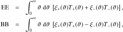 (6)Under the condition that
 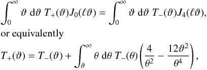 (7)EE only contains E-modes, BB only B-modes. One can also define a mixed-term EB which is derivable from a mixture of E- and B-modes ⟨ψEψB ⟩, and observable as the imaginary part of ξ−. However, this EB term violates parity. It generally vanishes since the shear field is expected to be parity symmetric.
E-/B-mode separation needs to be performed separately at each statistical order. The general approach to constructing E-/B-separating statistics remains the same for higher-order statistics, only the conditions for the weight functions that connect the shear correlation functions to the E-/B-separating statistics need to be individually derived at each order. For third-order statistics, the conditions for general E-/B-mode separation are given in Shi et al. (2011).
2.2. Aperture mass statistics
The aperture mass Map was first introduced by Kaiser (1995) and Schneider (1996) to estimate masses of galaxy clusters from gravitational lensing signals. It is a filtered version of both the shear γ and the real part of the convergence, κE ≡ ∇2ψE / 2 with axisymmetric filter functions, ![Mathematical equation: \begin{eqnarray} \label{eq:mapdef} M_{\rm ap}(\theta) &=& \int \dd^2 r \; Q_{\theta}(|\vek{r}|)\; \gamma_{\rm t}(\vek{r}) \nonumber\\[-1mm] &=&\int \dd^2 r \; U_{\theta}(|\vek{r}|)\; \kappa_E(\vek{r}) , \end{eqnarray}](/articles/aa/full_html/2014/01/aa22605-13/aa22605-13-eq27.png) (8)with tangential shear γt being specified relative to the center of the aperture. The function Uθ is an compensated filter function, and the filter functions Uθ and Qθ are inter-related by the relation
(8)with tangential shear γt being specified relative to the center of the aperture. The function Uθ is an compensated filter function, and the filter functions Uθ and Qθ are inter-related by the relation 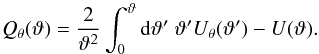 (9)The two most often used sets of filter function forms, the polynomial one proposed by Schneider et al. (1998), and the exponential one by Crittenden et al. (2002), have (nearly) finite support in both real and Fourier space. This feature makes the variance of aperture mass
  useful also in cosmic shear studies. This statistic provides a well-localized probe of the power spectrum and is easy to determine from observational data.
Tangential shear averaged over a circle is only sensitive to E-modes, whereas cross shear over a circle is only sensitive to B-modes. Therefore the aperture mass Map is a measure of the E-mode shear. A corresponding quantity, 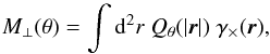 (10)accordingly is a measure of the B-mode shear.
At the three-point level, it is convenient to combine the eight correlation functions into the natural components (Schneider & Lombardi 2003) 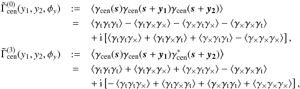 (11)where γcen is defined relative to the center of mass of the triangle characterized with two side lengths y1,y2 and the angle between them φy (see Fig. 1). Because they are measured relative to a center of the triangle formed by the three positions of shear measurements, these natural components are independent of the orientation of the triangle.
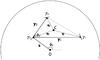 |
Fig. 1 Sketch of the halo model (1-halo term) for shear three-point functions and the notations used. In the text, the three shears in three-point shear correlator e.g. ⟨γγγ ⟩ correspond to γ1, γ2, and γ3, accordingly. Note that the polar angle of any vector k in Cartesian coordinates is denoted as φk, but φy is defined to be the angle between y1 and y2. |
Jarvis et al. (2004) and Schneider et al. (2005) have derived the relations between the natural components of the shear three-point functions (shear 3PCFs) and the aperture mass statistics using the Crittenden et al. (2002) filter functions 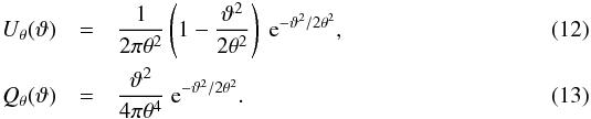 Here we present the relations in the specific case of three equal filter sizes, and refer to Eqs. (62), (68) and (73) in Schneider et al. (2005) for the general form:
 ![Mathematical equation: \begin{eqnarray} \label{eq:map_3} \ba{M_{\rm ap}^3}(\theta) &\;=\;& \frac{1}{4}\int_0^{\infty} \frac{\dd y_1 y_1}{\theta^2} \int_0^{\infty} \frac{\dd y_2 y_2}{\theta^2} \int_0^{2\pi} \frac{\dd \phi_y}{2\pi}\, \nonumber\\ & & \Re\; \Bigl[ 3 \tilde{\Gamma}_{\rm cen}^{(3)}(y_1,y_2,\phi_y) T_3(\theta,y_1,y_2,\phi_y) \nonumber\\ && + \tilde{\Gamma}_{\rm cen}^{(0)}(y_1,y_2,\phi_y) T_0(\theta,y_1,y_2,\phi_y) \Bigr] \end{eqnarray}](/articles/aa/full_html/2014/01/aa22605-13/aa22605-13-eq47.png) (14)is the pure E-mode (EEE) statistics, with
(14)is the pure E-mode (EEE) statistics, with 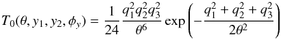 (15)and
 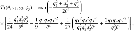 (16)where qi indicates the vectors pointing from the center of mass of the triangle (y1,y2,φy) to its vertices (see Fig. 1),
  (17)Here we used a complex notation so that a vector (a,b) corresponds to the complex number q = a + ib. The asterisk denotes the complex conjugation, so q∗ = a − ib corresponds to the vector (a, − b). For the forms of the weight functions T0,3, a Gaussian filter was assumed. Without loss of generality, we choose y1 to be parallel to the x-axis, so that φy1 = 0 and φy is the polar angle of y2.
Similarly, the B-mode three-point aperture mass statistics include the EEB term ![Mathematical equation: \begin{eqnarray} \ba{M_{\rm ap}^2 M_{\perp}}(\theta)& =& \frac{1}{4}\int_0^{\infty} \frac{\dd y_1 y_1}{\theta^2} \int_0^{\infty} \frac{\dd y_2 y_2}{\theta^2} \int_0^{2\pi} \frac{\dd \phi_y}{2\pi}\, \nonumber \\ &&\Im\; \Bigl[ \tilde{\Gamma}_{\rm cen}^{(3)}(y_1,y_2,\phi_y) T_3(\theta,y_1,y_2,\phi_y)\nonumber \\ && +\tilde{\Gamma}_{\rm cen}^{(0)}(y_1,y_2,\phi_y) T_0(\theta,y_1,y_2,\phi_y) \Bigr] , \end{eqnarray}](/articles/aa/full_html/2014/01/aa22605-13/aa22605-13-eq61.png) (18)the EBB term
(18)the EBB term ![Mathematical equation: \begin{eqnarray} \label{eq:EBB} \ba{M_{\rm ap} M_{\perp}^2}(\theta)& = & \frac{1}{4}\int_0^{\infty} \frac{\dd y_1 y_1}{\theta^2} \int_0^{\infty} \frac{\dd y_2 y_2}{\theta^2} \int_0^{2\pi} \frac{\dd \phi_y}{2\pi}\,\nonumber\\ && \Re \; \Bigl[ \tilde{\Gamma}_{\rm cen}^{(3)}(y_1,y_2,\phi_y) T_3(\theta,y_1,y_2,\phi_y)\nonumber\\ &&-\tilde{\Gamma}_{\rm cen}^{(0)}(y_1,y_2,\phi_y) T_0(\theta,y_1,y_2,\phi_y)\Bigr] , \end{eqnarray}](/articles/aa/full_html/2014/01/aa22605-13/aa22605-13-eq62.png) (19)and the BBB term
(19)and the BBB term ![Mathematical equation: \begin{eqnarray} \label{eq:BBB} \ba{M_{\perp}^3}(\theta) &=& \frac{1}{4}\int_0^{\infty} \frac{\dd y_1 y_1}{\theta^2} \int_0^{\infty} \frac{\dd y_2 y_2}{\theta^2} \int_0^{2\pi} \frac{\dd \phi_y}{2\pi} \nonumber\\ && \Im \;\Bigl[ 3 \tilde{\Gamma}_{\rm cen}^{(3)}(y_1,y_2,\phi_y) T_3(\theta,y_1,y_2,\phi_y) \nonumber\\ &&-\tilde{\Gamma}_{\rm cen}^{(0)}(y_1,y_2,\phi_y) T_0(\theta,y_1,y_2,\phi_y)\Bigr] . \end{eqnarray}](/articles/aa/full_html/2014/01/aa22605-13/aa22605-13-eq63.png) (20)Among them,
(20)Among them,  and
and  violate parity, whereas
  conserves parity symmetry and therefore is harder to distinguish from pure E-mode statistics.
3. E-/B-mode mixing with three-point aperture mass statistics
Here we investigate the degree of EB-mixing in three-point aperture mass statistics due to the aforementioned small-scale information loss. Since three-point statistics probe more into the nonlinear, small-scale regime than their two-point counterparts, one might naively expect three-point statistics to be more severely affected by the small-scale information loss.
We follow these steps: (i) we model the “observable” shear 3PCFs which contain only E-mode signal; (ii) we derive the aperture statistics from the shear 3PCFs; (iii) we introduce a cutoff in the 3PCFs at a small angular scale, mimicking the effect of information loss due to unreliable shear estimates caused by overlapping galaxy images (this generates a B-mode signal that results in a nonzero B-mode aperture statistic that conserves parity), and we repeat step (ii) using only correlation functions above the cutoff scale; (iv) finally, we compare the aperture mass statistics resulted from steps (ii) and (iii).
3.1. Modeling
We use the real-space halo model (Zaldarriaga & Scoccimarro 2003; Takada & Jain 2003b) to model shear three-point correlation functions. Since our study focuses on small scales, the halo model is a natural choice because it is expected to provide the most precise predictions on small scales. For the same reason, slightly imprecise modeling on large scales will not affect our main results. We take advantage of this and neglect the two- and three-halo terms, which significantly reduces the computational load. In fact, as shown by Takada & Jain (2003b), the one-halo term already captures most of the features of the shear 3PCFs measured from ray-tracing simulations.
In the real-space halo model the convergence profile for a halo of mass M can be expressed as  (21)where s is the angular distance from the center of the halo, fK indicates the comoving angular diameter distance, a is the scale factor, and χ and χs are the comoving distance to the halo and the source, respectively. The surface mass density Σ contributed by the halo is computed from an NFW profile ρNFW (Navarro et al. 1996) with cutoff at the virial radius rvir
 (22)where r∥ is the proper distance along the line of sight. Σ can be expressed analytically,
  (23)with ch being the halo concentration parameter, and θvir(M,χ) = rvir(M,χ) / fK(χ) / a(χ). The explicit form of the function F(x) is given by Eq. (27) in Takada & Jain (2003a).
The halo model tangential shear profile can then be expressed using the relation  (24)with
  being the mean surface mass density inside a circle of radius s. The tangential shear profile can also be expressed analytically as
 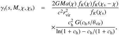 (25)see Eq. (17) in Takada & Jain (2003b) for the explicit form of the function G(x). Note that comoving coordinates have been used to express the surface mass density and the distances in Takada & Jain (2003a,b).
The natural components of shear 3PCFs can then be derived by averaging shear triplets over the triangle angular position s, and summing contributions from all halos with a comoving distance χ smaller than that of the source χs (see also Takada & Jain 2003a),
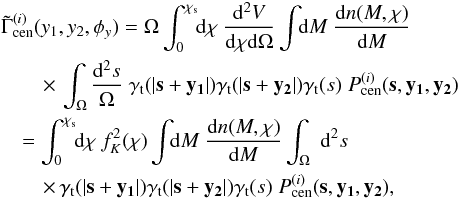 (26)
(26)
where Ω is the angular coverage of the full sky, V is the comoving volume element, and n is the comoving halo mass function. We have taken the form of the comoving differential volume  , which is true for a flat universe. Again we chose y1 to be parallel to the x-axis. This does not affect generality since the last integral does not depend on φy1 because of the spherical symmetry of a halo. The mass and distance dependencies of γt are not shown to keep the notation concise. We define
  to be the projection operator for
  , which projects the three shears (or their complex conjugates) measured relative to the center of the halo to those measured relative to the center of mass of the triangle formed by y1 and y2 (see Fig. 1). To derive its form, we first consider the projection of one of the shears, for example, γ3. The shear value γ(s) can be seen as γ3 measured relative to the center of the halo. Using Eq. (3), one can express γ3 in Cartesian coordinates and then project it relative to the center of mass of the triangle
 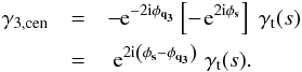 (27)Taking the definition of the natural components (11) into account, the explicit form of
  reads
reads 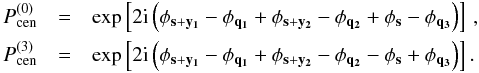 (28)The different polar angles can be expressed as functions of s, y1 and y2.
We adopt a flat ΛCDM cosmology with dark matter content Ωm0 = 0.28, dark energy content ΩΛ = 0.72, Hubble parameter h0 = 0.7, slope of the initial power spectrum ns = 0.96, and the normalization of the matter power spectrum σ8 = 0.8. We use the Tinker et al. (2008) formula to model the halo mass function, and the Duffy et al. (2008) fitting formula for the concentration parameter of NFW halos. To reduce the computational load even more, we assume a single plane of source galaxies at redshift zs = 1 (see the discussion section for a generalization from this case).
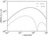 |
Fig. 2 Dependence of the modeled shear 3PCFs on angular separation. The two parity-invariant components ttt (stands for ⟨γtγtγt ⟩) and × ×t (stands for ⟨γ×γ×γt ⟩) are shown for equilateral triangles, see Eq. (11). The × ×t signal becomes negative beyond r ≈ 2 arcmin, and its absolute value is plotted for larger angles. |
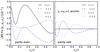 |
Fig. 3 Dependence of the modeled shear 3PCFs on triangle configuration. A subset of triangle configurations with two equal side-lengths y1 = y2 = 1 arcminute is shown, and plotted are the dependencies of the shear 3PCFs on the angle between them. The left panel “parity even” shows shear 3PCFs that involve zero or two tangential shears and are thus invariant under a parity transformation, while the right panel shows shear 3PCFs that contain an odd number of tangential shears and therefore change sign under parity transformation. The notation in the labels is analogous to Fig. 2. |
Figures 2 and 3 present the modeled shear three-point correlation functions. Shown are the three-point correlators of shear components that can be seen as parts of the natural components, see (11). As can be seen from Fig. 2, the pure tangential component ⟨γtγtγt ⟩ peaks at about 30 arcsec for equilateral triangle configurations. In comparison, the virial radius for a 1014 M⊙ halo at z = 0.5 corresponds to an angular size of approximately 100 arcsec. In contrast to shear 2PCFs, all shear 3PCFs vanish when r → 0. This is expected since a statistically isotropic spin-2 field has vanishing skewness. For equilateral triangles, ⟨γ×γ×γt⟩ = ⟨γ×γtγ×⟩ = ⟨γtγ×γ× ⟩, and all the components involving 1 or 3 γ× vanish, owing to the additional symmetry of three equal side-lengths. Therefore only two components are plotted in Fig. 2.
Figure 3 shows a strong dependence of shear 3PCFs on the triangle shape. After taking account of the different ordering of the three shears and the different definitions of φ, the shapes are consistent with Fig. 6 in Zaldarriaga & Scoccimarro (2003). The detailed shapes of the curves are difficult to understand in detail, but several features do appear as expected. First, for equilateral triangles (φy = π / 3) one sees the additional symmetry ⟨γ×γ×γt⟩ = ⟨γ×γtγ×⟩ = ⟨γtγ×γ× ⟩ and ⟨γ×γtγt⟩ = ⟨γtγ×γt⟩ = ⟨γtγtγ× ⟩. Second, because we plotted isosceles triangles, for all opening angles ⟨γ×γtγ×⟩ = ⟨γtγ×γ× ⟩, ⟨γ×γtγt⟩ = − ⟨γtγ×γt ⟩, and ⟨γtγtγ×⟩ = ⟨γ×γ×γ×⟩ = 0. Third, for collapsed triangles (θ = 0), the ⟨γtγtγt ⟩ and ⟨γ×γ×γt ⟩ components have the same sign. This is expected since for collapsed triangles two of the three shear components have the same value and thus their product is always positive. The sign of the shear 3PCF then depends on the third shear component, which is shared by ⟨γtγtγt ⟩ and ⟨γ×γ×γt ⟩. Judging from this feature, some of the shear 3PCFs in Fig. 10 in Takada & Jain (2003b) have incorrect signs. Apart from that figure shows the same dependencies of the shear 3PCFs. Finally, the triangle configuration with opening angle φy = ψ and that with φy = −ψ can be considered as mirror images of each other, so are the triangle configuration with opening angle φy = π − ψ and that with φy = π + ψ. This implies that γ3PCF(y1,y2,ψ) = γ3PCF(y1,y2, − ψ) = γ3PCF(y1,y2,2π − ψ) when γ3PCF is a parity-even shear 3PCF, and therefore the slopes of the parity-even shear 3PCFs at φy = 0 and φy = π are zero; on the other hand, γ3PCF(y1,y2,ψ) = −γ3PCF(y1,y2, − ψ) = −γ3PCF(y1,y2,2π − ψ) when γ3PCF is a parity-odd shear 3PCF, and the shear 3PCF values at φ = 0 and φ = π for parity-odd shear 3PCFs are zero, as shown in the figure.
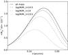 |
Fig. 4 Three-point aperture mass statistic |
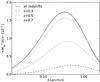 |
Fig. 5 Same as Fig. 4, but showing contributions from halos below different redshift limits. The line with “all redshifts” contains contributions from all halos below the source redshift zs = 1. |
The modeled third-order aperture mass statistic  under different mass and redshift cuts are presented in Figs.4 and 5. Since only the one-halo term is considered in the model, the contributions from different halos to the signal are additive. The dominant contribution to the signal on and above arcminute scales comes from z = 0.3 to z = 0.7, and from massive halos corresponding to galaxy groups and clusters. In particular, when the filter scale is larger than 80 arcsec, more than half of the signal is contributed by halos with masses larger than 1014 M⊙. The peak of the signal is located at θ ≈ 20 arcsec. The signal at larger aperture radii is dominated by larger halos at lower redshifts. Therefore the signal shifts to lower θ as an upper mass cutoff is introduced, and to higher θ as an upper redshift cutoff is introduced.
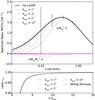 |
Fig. 6 E-/B-mode mixing with three-point aperture mass statistics due to small-scale cutoff at θmin = 1, 2 and 5 arcsec. In the upper panel, the black lines represent the E-mode aperture mass statistic |

3.2. Effect of small-scale cutoff
As described in Kilbinger et al. (2006), the small-scale information loss is attributed to the fact that the shapes of close galaxy pairs cannot be estimated reliably (see also the detailed discussion in Miller et al. 2013). The angular scale below which this information loss occurs depends on the true angular sizes of galaxies, on the point spread function of the observation, and the ability of the shear measurement algorithm to separate overlapping isophotes. The typical size of this cutoff used in current shear measurement methods is a few arcseconds for space-based observations (e.g. 3 arcsec in the COSMOS analysis of Schrabback et al. 2010), and slightly larger scales for ground-based observations (e.g. 9 arcsec in CFHTLenS as discussed in Kilbinger et al. 2013).
We introduce a small angular scale cutoff in the three-point correlation function at 1, 2, 5, and 10 arcsec, and show the E-/B-mode mixing introduced into the aperture mass statistics  and
and  in Fig. 6.
As expected, small-scale information loss leads to a decrease in the E-mode aperture mass signal , and introduces a spurious parity-conserving B-mode signal . The parity-violating B-mode signals are consistent with zero over all angular scales, both with and without cutoff. This is expected since aperture mass statistics are computed over shear correlation functions with triangle configurations of both parities.
Somewhat surprisingly, the decrease in the E-mode aperture mass signal due to a small-scale cutoff is less significant for third-order statistics than at second order (see Fig. 1 of Kilbinger et al. 2006). The angular scales that are significantly affected are below 10θmin. This means that even for a conservative small-scale cutoff at 10 arcsec, the effect is limited to ≲arcmin scales. Since these scales are strongly influenced by complicated baryonic physics which prevents precise theoretical predictions, signals on these small scales are usually not used to infer cosmology. At second-order, however, the decrease at 1 arcmin angular separation can be as high as 10% for θmin = 5 arcsec, compared to <0.5% at the third-order with the same cutoff scale. This difference can be understood by comparing the relations between aperture mass statistics and shear correlations function for the second- and third-order case. In the former case, one of the two correlation functions ξ+ and its corresponding weight function T+ both peak at zero angular separation. In contrast, none of the shear 3PCFs peak at small scales, and both weight functions T0 and T3 vanish when θ approaches 0. Accordingly, a small-scale cutoff in the three-point shear correlation functions causes a weaker effect on the aperture mass statistics.
Leakage to B-modes is even weaker than the decrease in E-mode signal. This is also very different from the two-point case, where the growth in the B-mode signal on small scales due to a cutoff approximately equals the decrease in E-mode signal in size. This small leakage enables the parity conserving B-mode to remain a good test for systematics in third-order statistics even in the presence of a small-scale cutoff in the 3PCFs.
At the small angular scales where the E-/B-mode mixing occurs, shot or shape noise (the noise due to randomness of the intrinsic shapes of the galaxies) is the major source of uncertainty in the measurement of the aperture mass signals. We plot in Fig. 6 the shape noise contribution (see appendix) to the uncertainty of for the Euclid survey. The decrease in the E-mode aperture mass signal caused by a small-scale cutoff is subdominant to the uncertainty of measurement for θmin < 5 arcsec, even for a large and relatively deep survey like Euclid. For surveys with smaller sky coverage and/or shallower depth, the shot noise contribution is expected to be even higher. Therefore, the E-/B-mode mixing effect on the third-order statistics is generally not observable.
4. Discussion
As mentioned above, a single source-plane at z = 1 was used for this study. This source redshift was chosen to represent deep surveys like Euclid (which has an expected median source redshift of z ≈ 0.9). The results we obtained, however, can be generalized to shallower surveys as well. According to the halo model, if the comoving distance to the source χs is changed, the shear 3PCF contributed by a certain halo at χ changes its amplitude as [fK(χs − χ) / fK(χs)]3, whereas the angular dependence is retained (25, 26). A shallower survey will give more relative weight to low-redshift halos, which will shift the signals to larger angular scales (see e.g. Fig. 5), making slightly less affected by small-scale cutoff.
We have tested EB-mixing in third-order aperture statistics with three equal-sized filters. For the more general case with three different filter sizes, that is  , we argued that the degree of EB-mixing is bounded from above by that for
  , with θ1 being the smallest of the three filter sizes. To see this, it is helpful to consider the aperture mass as obtained by placing apertures on the image. In this case, the estimator of involves summation over all galaxy triplets in the field, with the three galaxies in a triplet being weighted by three different filters. A small-scale cutoff will eliminate close triplets from this sum and cause the E-mode signal to be underestimated. This underestimation is most severe when all three galaxies in the triplet are given high weights from their corresponding filters. Because the filter Qθ is more extended for a larger filter size θ, the eliminated close triplets are on average given a lower weight relative to the retained ones when some of the filter sizes are larger in size. Therefore, if EB-mixing is negligible in at θ1, it is also negligible in a general aperture mass statistic with θ2 ≥ θ1 and θ3 ≥ θ1.
The test we performed shows how much E-mode signal will leak to the B-mode under a small-scale cutoff for third-order aperture statistics. The opposite question needs to be addressed in a quantitative way as well: if there exists a B-mode signal, for instance, from noise and bias coming from shape measurements or intrinsic alignments of galaxy shapes, how much will the E-mode signal be affected? The answer to this question depends on the actual angular and shape dependencies of the particular B-mode contamination and is therefore hard to give in general. For future lensing surveys, once the amplitude of the B-mode signal and its statistical uncertainty is known, one can study the maximum bias a small-scale cutoff could contribute to the E-mode signal. Ultimately, each contribution to both E- and B-mode signals needs to be understood to derive precise cosmological information from cosmic shear measurements.
5. Conclusion
We tested the degree of EB-mixing in third-order aperture statistics due to the inevitable absence of small-scale correlation measurements. Both the decrease in E-mode signal and the introduction of a spurious B-mode signal were found to be smaller for the third-order aperture mass statistics than for the second-order ones. Quantitatively, the change in the E-mode signal is lower than 1% at an angular separation of ten times the cutoff scale and above, and therefore is negligible on angular scales of interest to ongoing and future weak lensing surveys. Some parity-preserving B-mode signal is created on small angular scales (<1 arcmin) because of the small-scale cutoff, but with an amplitude that is even smaller than the decrease in the E-mode signal. The parity-violating B-modes remain zero in the presence of a small-scale cutoff.
These findings suggest that the aperture statistics introduce only negligible E-/B-mode mixing for third-order shear statistics on the angular scales that will be probed by ongoing and future weak lensing surveys. Therefore, third-order aperture statistics can safely be used as E-/B-mode separating statistics to infer cosmological information from those surveys.
Acknowledgments
We thank Martin Kilbinger for helpful discussions, and Masahiro Takada for his quick email response regarding their halo model paper (Takada & Jain 2003b). This work was supported by the Deutsche Forschungsgemeinschaft under the project B5 in the TRR33 “The Dark Universe”. B.J. acknowledges support by an STFC Ernest Rutherford Fellowship, grant reference ST/J004421/1.
References
- Abdalla, F. B.,Amara, A.,Capak, P., et al. 2008, MNRAS, 387, 969 [NASA ADS] [CrossRef] [Google Scholar]
- Asgari, M.,Schneider, P., &Simon, P. 2012, A&A, 542, A122 [NASA ADS] [CrossRef] [EDP Sciences] [Google Scholar]
- Crittenden, R. G.,Natarajan, P.,Pen, U., &Theuns, T. 2002, ApJ, 568, 20 [NASA ADS] [CrossRef] [Google Scholar]
- Duffy, A. R., Schaye, J., Kay, S. T., & Dalla Vecchia, C. 2008, MNRAS, 390, L64 [NASA ADS] [CrossRef] [Google Scholar]
- Eifler, T.,Schneider, P., &Krause, E. 2010, A&A, 510, A7 [NASA ADS] [CrossRef] [EDP Sciences] [Google Scholar]
- Fu, L., &Kilbinger, M. 2010, MNRAS, 401, 1264 [NASA ADS] [CrossRef] [Google Scholar]
- Hilbert, S.,Hartlap, J.,White, S. D. M., &Schneider, P. 2009, A&A, 499, 31 [NASA ADS] [CrossRef] [EDP Sciences] [Google Scholar]
- Hu, W., &White, M. 1997, Phys. Rev. D, 56, 596 [NASA ADS] [CrossRef] [Google Scholar]
- Huterer, D.,Takada, M.,Bernstein, G., &Jain, B. 2006, MNRAS, 366, 101 [NASA ADS] [CrossRef] [Google Scholar]
- Jarvis, M.,Bernstein, G., &Jain, B. 2004, MNRAS, 352, 338 [NASA ADS] [CrossRef] [Google Scholar]
- Joachimi, B.,Shi, X., &Schneider, P. 2009, A&A, 508, 1193 [NASA ADS] [CrossRef] [EDP Sciences] [Google Scholar]
- Kaiser, N. 1995, ApJ, 439, L1 [NASA ADS] [CrossRef] [Google Scholar]
- Kamionkowski, M.,Kosowsky, A., &Stebbins, A. 1997, Phys. Rev. D, 55, 7368 [NASA ADS] [CrossRef] [Google Scholar]
- Kamionkowski, M.,Babul, A.,Cress, C. M., &Refregier, A. 1998, MNRAS, 301, 1064 [NASA ADS] [CrossRef] [Google Scholar]
- Kayo, I., & Takada, M. 2013 [arXiv:1306.4684] [Google Scholar]
- Kayo, I.,Takada, M., &Jain, B. 2013, MNRAS, 429, 344 [NASA ADS] [CrossRef] [Google Scholar]
- Kilbinger, M.,Schneider, P., &Eifler, T. 2006, A&A, 457, 15 [Google Scholar]
- Kilbinger, M.,Fu, L.,Heymans, C., et al. 2013, MNRAS, 430, 2200 [NASA ADS] [CrossRef] [Google Scholar]
- Kitching, T. D.,Balan, S. T.,Bridle, S., et al. 2012, MNRAS, 423, 3163 [NASA ADS] [CrossRef] [Google Scholar]
- Krause, E.,Schneider, P., &Eifler, T. 2012, MNRAS, 423, 3011 [NASA ADS] [CrossRef] [Google Scholar]
- Laureijs, R., Amiaux, J., Arduini, S., et al. 2011 [arXiv:astro-ph/1110.3193] [Google Scholar]
- Miller, L.,Heymans, C.,Kitching, T. D., et al. 2013, MNRAS, 429, 2858 [Google Scholar]
- Navarro, J. F.,Frenk, C. S., &White, S. D. M. 1996, ApJ, 462, 563 [NASA ADS] [CrossRef] [Google Scholar]
- Pen, U.-L.,Zhang, T., van Waerbeke, L., et al. 2003, ApJ, 592, 664 [NASA ADS] [CrossRef] [Google Scholar]
- Schneider, P. 1996, MNRAS, 283, 837 [NASA ADS] [CrossRef] [Google Scholar]
- Schneider, P., &Kilbinger, M. 2007, A&A, 462, 841 [NASA ADS] [CrossRef] [EDP Sciences] [Google Scholar]
- Schneider, P., &Lombardi, M. 2003, A&A, 397, 809 [NASA ADS] [CrossRef] [EDP Sciences] [Google Scholar]
- Schneider, P., van Waerbeke, L.,Jain, B., &Kruse, G. 1998, MNRAS, 296, 873 [NASA ADS] [CrossRef] [Google Scholar]
- Schneider, P., van Waerbeke, L., &Mellier, Y. 2002, A&A, 389, 729 [NASA ADS] [CrossRef] [EDP Sciences] [Google Scholar]
- Schneider, P.,Kilbinger, M., &Lombardi, M. 2005, A&A, 431, 9 [NASA ADS] [CrossRef] [EDP Sciences] [Google Scholar]
- Schneider, P.,Eifler, T., &Krause, E. 2010, A&A, 520, A116 [NASA ADS] [CrossRef] [EDP Sciences] [Google Scholar]
- Schrabback, T.,Hartlap, J.,Joachimi, B., et al. 2010, A&A, 516, A63 [NASA ADS] [CrossRef] [EDP Sciences] [Google Scholar]
- Semboloni, E.,Heymans, C., van Waerbeke, L., &Schneider, P. 2008, MNRAS, 388, 991 [NASA ADS] [CrossRef] [Google Scholar]
- Semboloni, E.,Schrabback, T., van Waerbeke, L., et al. 2011, MNRAS, 410, 143 [NASA ADS] [CrossRef] [Google Scholar]
- Shi, X.,Joachimi, B., &Schneider, P. 2010, A&A, 523, A60 [NASA ADS] [CrossRef] [EDP Sciences] [Google Scholar]
- Shi, X.,Schneider, P., &Joachimi, B. 2011, A&A, 533, A48 [Google Scholar]
- Stebbins, A. 1996, unpublished [arXiv:astro-ph/9609149] [Google Scholar]
- Takada, M., &Jain, B. 2003a, MNRAS, 340, 580 [NASA ADS] [CrossRef] [Google Scholar]
- Takada, M., &Jain, B. 2003b, MNRAS, 344, 857 [NASA ADS] [CrossRef] [Google Scholar]
- Takada, M., &Jain, B. 2004, MNRAS, 348, 897 [NASA ADS] [CrossRef] [Google Scholar]
- Tinker, J.,Kravtsov, A. V.,Klypin, A., et al. 2008, ApJ, 688, 709 [NASA ADS] [CrossRef] [Google Scholar]
- Van Waerbeke, L.,Mellier, Y.,Erben, T., et al. 2000, A&A, 358, 30 [NASA ADS] [Google Scholar]
- Zaldarriaga, M., &Scoccimarro, R. 2003, ApJ, 584, 559 [NASA ADS] [CrossRef] [Google Scholar]
- Zaldarriaga, M., &Seljak, U. 1997, Phys. Rev. D, 55, 1830 [Google Scholar]
Appendix A: Shape noise contribution to the uncertainty of the  measurement
Here we derive a simple formula that yields an approximate estimate of  , the uncertainty of
  measurement contributed by the shape noise.
We consider first the measurement of within a single aperture of angular radius θ. A convenient estimator is 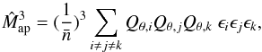 (A.1)where
  is the mean number density of galaxy images, and the sum runs over all triples of galaxy shapes in the aperture. This estimator resembles Eg. (5.24) of Schneider et al. (1998), but excludes the cases with two or three equal indices, for example, i = j. It is unbiased when the number of galaxies inside the aperture is very large.
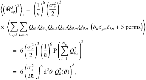
The shape noise contribution to the dispersion of measurements in this aperture is, by definition,  . Neglecting high-order correlations, the shape noise contribution to
  is
is
 (A.2)
(A.2)
where  is the average number of galaxies inside the aperture. In the second equation we substituted the ensemble average ⟨ ⟩ with an average over all possible galaxy positions (see Eq. (5.3) of Schneider et al. 1998),
  (A.3)With Crittenden et al. (2002) filter function Qθ (13), the integral in the last line of (A.2) has a value of 1 / (πθ2). This leads to
  (A.4)For a galaxy survey of size A, a number Nf of nearly independent apertures can be put on the field. This approximately reduces the uncertainty of measurement by a factor of
  . Using a rough estimation of Nf = A / (4θ2), we obtain
 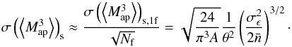 (A.5)We note again that this estimation of is aimed to be simple and approximate. Practically, is estimated not with (A.1) but is derived from the shear 3PCFs (14), or similarly, from the bispectrum of shear. This would lead to a slightly different prefactor in the expression of . For a more precise estimation of this prefactor, one can use Eq. (26) in Joachimi et al. (2009) as an estimate of the bispectrum covariance, and derive the covariance of with the help of Eq. (46) in Schneider et al. (2005).
All Figures
|
Fig. 1 Sketch of the halo model (1-halo term) for shear three-point functions and the notations used. In the text, the three shears in three-point shear correlator e.g. ⟨γγγ ⟩ correspond to γ1, γ2, and γ3, accordingly. Note that the polar angle of any vector k in Cartesian coordinates is denoted as φk, but φy is defined to be the angle between y1 and y2. |
| In the text | |
|
Fig. 2 Dependence of the modeled shear 3PCFs on angular separation. The two parity-invariant components ttt (stands for ⟨γtγtγt ⟩) and × ×t (stands for ⟨γ×γ×γt ⟩) are shown for equilateral triangles, see Eq. (11). The × ×t signal becomes negative beyond r ≈ 2 arcmin, and its absolute value is plotted for larger angles. |
| In the text | |
|
Fig. 3 Dependence of the modeled shear 3PCFs on triangle configuration. A subset of triangle configurations with two equal side-lengths y1 = y2 = 1 arcminute is shown, and plotted are the dependencies of the shear 3PCFs on the angle between them. The left panel “parity even” shows shear 3PCFs that involve zero or two tangential shears and are thus invariant under a parity transformation, while the right panel shows shear 3PCFs that contain an odd number of tangential shears and therefore change sign under parity transformation. The notation in the labels is analogous to Fig. 2. |
| In the text | |
|
Fig. 4 Three-point aperture mass statistic |
| In the text | |
|
Fig. 5 Same as Fig. 4, but showing contributions from halos below different redshift limits. The line with “all redshifts” contains contributions from all halos below the source redshift zs = 1. |
| In the text | |
|
Fig. 6 E-/B-mode mixing with three-point aperture mass statistics due to small-scale cutoff at θmin = 1, 2 and 5 arcsec. In the upper panel, the black lines represent the E-mode aperture mass statistic |
| In the text | |
Current usage metrics show cumulative count of Article Views (full-text article views including HTML views, PDF and ePub downloads, according to the available data) and Abstracts Views on Vision4Press platform.
Data correspond to usage on the plateform after 2015. The current usage metrics is available 48-96 hours after online publication and is updated daily on week days.
Initial download of the metrics may take a while.