| Issue |
A&A
Volume 561, January 2014
|
|
|---|---|---|
| Article Number | A140 | |
| Number of page(s) | 26 | |
| Section | Extragalactic astronomy | |
| DOI | https://doi.org/10.1051/0004-6361/201322486 | |
| Published online | 27 January 2014 | |
A low-luminosity type-1 QSO sample⋆
I. Overluminous host spheroidals or undermassive black holes?⋆⋆,⋆⋆⋆
1 I. Physikalisches Institut, Universität zu Köln, Zülpicher Str. 77, 50937 Köln, Germany
e-mail: This email address is being protected from spambots. You need JavaScript enabled to view it.
2 Deutsches Zentrum für Luft- und Raumfahrt (DLR), Königswinterer Str. 522-524, 53227 Bonn, Germany
3 Max-Planck-Institut für Radioastronomie, auf dem Hügel 69, 53121 Bonn, Germany
4 Observatoire de Paris, LERMA, 61 Av. de l’Observatoire, 75014 Paris, France
5 European Southern Observatory (ESO), Casilla 19001, Santiago 19, Chile
6 Leibniz-Institut für Astrophysik Potsdam (AIP), an der Sternwarte 16, 14482 Potsdam, Germany
Received: 14 August 2013
Accepted: 29 October 2013
Abstract
Recognizing the properties of the host galaxies of quasi-stellar objects (QSOs) is essential for understanding the suspected coevolution of central supermassive black holes (BHs) and their host galaxies. Low-luminosity type-1 QSOs (LLQSOs) are ideal targets because of their small cosmological distance, which allows for a detailed structural analysis. We selected a subsample of the Hamburg/ESO survey for bright UV-excess QSOs that contains only the 99 nearest QSOs with redshift z ≤ 0.06. From this LLQSO sample, we observed 20 galaxies and performed aperture photometry and bulge-disk-decomposition with BUDDA on near-infrared J-, H-, and K-band images to separate disk, bulge, bar, and nuclear component. From the photometric decomposition of these 20 objects and visual inspection of images of another 26, we find that ~50% of the hosts are disk galaxies and most of them (86%) are barred. Stellar masses, calculated from parametric models based on inactive galaxy colors, range from 2 × 10⁹ M⊙ to 2 × 10¹¹ M⊙ with an average mass of 7 × 10¹⁰ M⊙. Black hole masses measured from single-epoch spectroscopy range from 1 × 10⁶ M⊙ to 5 × 10⁸ M⊙ with a median mass of 3 × 10⁷ M⊙. In comparison with higher-luminosity QSO samples, LLQSOs tend to have lower stellar and BH masses. Moreover, in the effective radius vs. mean surface-brightness projection of the fundamental plane, they lie in the transition area between luminous QSOs and normal galaxies. This can be seen as additional evidence that they populate a region intermediate between the local Seyfert population and luminous QSOs at higher redshift. This region has not been well studied so far. Eleven LLQSOs, for which we have reliable morphological decompositions and BH mass estimations, lie below the published BH mass vs. bulge luminosity relations for inactive galaxies. This can partially be explained if one assumes that the bulges of active galaxies contain much younger stellar populations than the bulges of inactive galaxies. Another possibility would be that their BHs are undermassive. This might indicate that the growth of the host spheroid precedes that of the BH.
Key words: galaxies: active / quasars: general / galaxies: Seyfert
ASCII tables of the fit results are only available at the CDS via anonymous ftp to cdsarc.u-strasbg.fr (130.79.128.5) or via http://cdsarc.u-strasbg.fr/viz-bin/qcat?J/A+A/561/A140
Figure 15 is available in electronic form at http://www.aanda.org
Based on observations with ESO-NTT, proposal no. 083.B-0739.
© ESO, 2014
1. Introduction
There is wide agreement that every galaxy, or at least those with a considerable bulge component, hosts a central supermassive black hole (SMBH; e.g. Kormendy & Richstone 1995; Richstone 1998; Ho 1999). Over the past decades, masses of SMBHs have been measured by dynamical modeling and spatially resolved kinematics as well as by reverberation mapping and single-epoch spectroscopy. A tight correlation between black hole mass MBH and the velocity dispersion σ of the bulge component of the host galaxy has been established (Ferrarese & Merritt 2000; Gebhardt et al. 2000). Similar correlations with bulge luminosity and mass have been found (e.g. Magorrian et al. 1998; Marconi & Hunt 2003; Häring & Rix 2004). Others, with the bulge Sérsic index (definition in Sect. 3.1) for instance, are still under discussion (Graham & Driver 2007; Vika et al. 2012).
Tight correlations between central SMBH and the host galaxy (resp. their bulges) have been interpreted as manifestations of an SMBH-host galaxy coevolution. Sanders et al. (1988) established a merger-driven scenario from ultraluminous infrared galaxies (ULIRGs) to quasi-stellar objects (QSOs) and quiescent dead ellipticals. However, in the past years, the detection of SMBHs in bulgeless galaxies and the finding that a considerable amount of local spiral galaxies host a disk-like pseudobulge instead of a classical bulge (e.g. Kormendy & Kennicutt 2004; Gadotti 2009), shows that the picture of galaxy evolution is not yet complete.
In the local Universe (z ≲ 0.2), studies of thousands of objects have shown that in sources with active galactic nuclei (AGN), the star formation and SMBH accretion rates are related to each other and also to the age of the stellar population. The history of SMBH growth (corresponding to the quasar activity) and star formation in the Universe is similar (e.g., Madau et al. 1998; Heckman et al. 2004; Hopkins & Beacom 2006; Silverman et al. 2009; Aird et al. 2010, and references therein). Several other findings (see review of Kormendy & Ho 2013) support the assumption that AGN feedback is crucial for the evolution of galaxies, at least at past epochs. However, in this context, the role of AGN is still unclear. Thus, a key question is whether hosts of AGN are different from those of inactive galaxies. Furthermore, it is unclear whether they follow the same black hole−bulge relations, or if any deviations from these correlations are indicative of an early evolutionary stage or of an entirely different evolution process driven by secular evolution or major mergers (e.g., Graham & Li 2009; Kormendy et al. 2011; Graham 2012; Scott et al. 2013; Kormendy & Ho 2013).
Many studies have focused on nearby Seyfert galaxies with very moderate nuclear emission on the one hand, and on the analysis of global properties of large samples of powerful QSOs at higher redshift on the other hand. To fill the gap between these two approaches, we analyzed a sample of low-luminosity type-1 QSOs (LLQSOs) at low redshift. This sample contains the closest known bright AGN that are still close enough for spatially resolved observations and a detailed structural analysis of the host galaxies. These galaxies constitute the important link between the local, but less luminous AGN and the powerful QSOs at higher redshifts (z ≥ 0.5). The detailed study of the hosts of type-1 QSOs is challenging because of the high contrast between the bright nuclear point source and the faint host.
The Hamburg/ESO Survey (HES, Wisotzki et al. 2000) is a wide-angle survey for optically bright QSOs and other rare objects in the southern hemisphere, covering a formal area of ≈9500 deg2 on the sky. A multitude of selection criteria are applied to select type-11 AGN up to z ≈ 3.2. The limiting magnitude is BJ < 17.3 with a dispersion of 0.5 mag between individual fields. The HES provides a methodologically complete sample of the local AGN population, that is, all AGN selected by the given criteria are included.
To select only the nearest AGN, we set a redshift limit of z = 0.06. This particular value was chosen to ensure the presence of the CO(2−0) band head in near-infrared (NIR) K-band spectra. This stellar absorption feature can be used to derive the stellar kinematics of the host galaxy or to analyze stellar populations (Gaffney et al. 1995; Fischer et al. 2006). These selection criteria result in a sample of 99 galaxies that we call the LLQSO sample throughout the text (for more information see Bertram et al. 2007). A redshift-magnitude diagram is shown in Fig. 1. The redshifts are taken from the HES. The magnitudes are nuclear BJ magnitudes (corresponding to the seeing disk) taken from the HES. The absolute magnitude range is −22.3 < MBJ < −16.8 with a median value of − 19.8. The median redshift is z = 0.043. The redshift-magnitude diagram shows that the selected galaxies lie below the commonly used division line of MB = −21.5 + 5log h0 between QSOs and Seyfert galaxies. Several galaxies from the LLQSO sample have been observed in molecular gas (CO, Bertram et al. 2007), atomic hydrogen (H i, König et al. 2009), and H2O-maser-emission (König et al. 2012). Fischer et al. (2006) studied nine galaxies in the NIR, focusing on spectroscopy.
In this work, we focus on structural and morphological properties of 20 galaxies (marked with squares in Fig. 1, object information in Table 1) that were randomly selected from the LLQSO sample. Our aim is to compare the properties of the hosts of these AGN with those of brighter QSOs and those of inactive galaxies. We analyze images in the NIR J-, H-, and K-band because these are less affected by dust extinction (AH/AV ≈ 0.175, Rieke & Lebofsky 1985). Furthermore, they are less affected by recent star formation and mainly trace intermediate-to-old (age ≳108 yr) red stars that dominate the stellar mass. Additionally, the contrast between the nuclear point source and the host galaxy has a minimum in the NIR (McLeod 1997). In Sect. 2, we report on the details of the observations as well as on the data reduction and calibration.
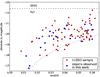 |
Fig. 1 Redshift-magnitude diagram of the 99 LLQSOs. The galaxies that have been observed and analyzed in this work are marked with squares. The limiting magnitude (BJ ≤ 17.3) of the HES is marked by the dashed-dotted line. |
We performed a detailed structural analysis with bulge-disk-bar-AGN decomposition using Budda and a photometric analysis of high-quality NIR images. The methods used for decomposition and photometry are described in Sect. 3. We estimated host stellar masses and bulge luminosities and compare them with other samples in the literature. In agreement with previous studies of type-1 AGN in the optical (e.g., Nelson et al. 2004; Kim et al. 2008; Bennert et al. 2011), the LLQSOs examined here do not follow the published black hole mass (MBH) vs. bulge luminosity (Lbulge) relations of inactive galaxies. In Sect. 4, we discuss possible reasons for the observed discrepancy. Summary and conclusions are presented in Sect. 5. Throughout this paper, we use a standard cosmological model with H0 = 70 km s-1 Mpc-1, Ωm = 0.3 and ΩΛ = 0.7.
Object information for the observed galaxies.
2. Observation, reduction, and calibration
In this study we used a set of thirteen galaxies drawn from the LLQSO sample that has been observed in the J-, H-, and Ks-band with the Son of ISAAC (SofI) infrared spectrograph and imaging camera on the New Technology Telescope (NTT, La Silla, Chile) during September 2009. The 1024 × 1024 Hawaii HgCdTe array provides a pixel scale of 0.288″/pixel with a field of view of 4.9 × 4.9 arcmin2.
Seven additional galaxies have been observed in the J-, H-, and Ks-band with the LBT NIR Spectrograph Utility with Camera and Integral-Field Unit for Extragalactic Research (LUCI) at the Large Binocular Telescope (LBT, Mt. Graham, USA) during May 2011 in seeing-limited mode. The 2048 × 2048 Rockwell Hawaii-2 HdCdTe array provides a pixel scale of 0.12″/pixel with a field of view of 4 × 4 arcmin2.
All images were obtained in jitter mode. Initially, flat-fielding (twilight-flat) and bad-pixel-correction were applied. The sky background was then removed by subtracting consecutive frames from each other. After aligning the resulting frames, a median frame was created. The images were flux calibrated using data from the 2 Micron All Sky Survey (2MASS) for foreground stars. Comparing the results of different stars, we can estimate that the calibration error is not higher than 10%.
We determined the seeing by fitting Gaussians to unresolved objects (stars) in the images. We present the average full width at half maximum (FWHM) of the fitted stars as measure of the seeing in Table 1. The seeing was around 1″ in most cases. To determine the depth of the observations, we measured the standard deviation σsky of the sky-subtracted background. We then calculated the mean 1σ sky deviation surface brightness ![Mathematical equation: \begin{equation} \sigma_\mathrm{sky} = -2.5 \log(\sigma[\mathrm{counts}]) + \mathrm{ZP} + 5 \log(\mathrm{pixel~scale}). \end{equation}](/articles/aa/full_html/2014/01/aa22486-13/aa22486-13-eq91.png) (1)The calculated values are presented in Table 1 as well and indicate a high sensitivity.
(1)The calculated values are presented in Table 1 as well and indicate a high sensitivity.
Parameters of the galaxies in the J-band.
Parameters of the galaxies in the H-band.
Parameters of the galaxies in the K-band.
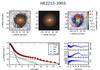 |
Fig. 2 Example of decomposition with Budda. We show (from left to right) the original H-band image, the model and the residuum (galaxy/model). Blue indicates regions where the model is fainter than the galaxy, red indicates regions where the model is brighter than the galaxy. In the lower row, we show an elliptically averaged radial profile of the galaxy, the single components, and the whole model. In the ellipse fits of the model, ellipticity and position angle are fixed as those of the original image. Furthermore, we show the difference between galaxy and model, ellipticity and position angle. |
3. Results
We describe the methods used for the surface-brightness decomposition, the tests we developed to establish the accuracy of such procedure and the derived results. Some relevant information about the studied sources is also summarized.
3.1. Decomposition
We used Budda2 (Bulge/Disk Decomposition Analysis) to perform the two-dimensional decomposition of the near-infrared galaxy images. Budda was developed by de Souza, Gadotti and dos Anjos and has been made publicly available (de Souza et al. 2004; Gadotti 2008).
We assumed the disk component to be fitted best by an exponential function (Freeman 1970) 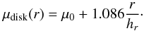 (2)Here, μ0 denotes the central surface brightness of the disk component and hr the characteristic scale length.
Furthermore, we used the Sérsic-function (Sérsic 1968) ![Mathematical equation: \begin{equation} \mu (r) = \mu_{\rm e} + c_n \left[ \left( \frac{r}{r_{\rm e} }\right)^{1/n} -1 \right] \end{equation}](/articles/aa/full_html/2014/01/aa22486-13/aa22486-13-eq99.png) (3)to fit bulges and bars. In the past, the bulge component has often been modeled with a Sérsic-profile with an index fixed to n = 4 (the so-called de Vaucouleurs-profile, see de Vaucouleurs (1948)). However, it has been shown that letting the Sérsic index of the bulge vary leads to better results (e.g. Gadotti 2009). For n = 1, the profile reduces to an exponential function. Even bars can be modeled with a Sérsic-index between ≈0.5 and ≈1.0 (Gadotti 2008). In the formula, re denotes the effective radius, that is, the radius that contains half of the fitted components’ flux, μe is the effective surface brightness, that is, the surface brightness at the effective radius. n is the Sérsic index and cn a parameter that depends on n: cn = 2.5(0.868n − 0.142) (Caon et al. 1993).
(3)to fit bulges and bars. In the past, the bulge component has often been modeled with a Sérsic-profile with an index fixed to n = 4 (the so-called de Vaucouleurs-profile, see de Vaucouleurs (1948)). However, it has been shown that letting the Sérsic index of the bulge vary leads to better results (e.g. Gadotti 2009). For n = 1, the profile reduces to an exponential function. Even bars can be modeled with a Sérsic-index between ≈0.5 and ≈1.0 (Gadotti 2008). In the formula, re denotes the effective radius, that is, the radius that contains half of the fitted components’ flux, μe is the effective surface brightness, that is, the surface brightness at the effective radius. n is the Sérsic index and cn a parameter that depends on n: cn = 2.5(0.868n − 0.142) (Caon et al. 1993).
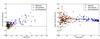 |
Fig. 3 Quality of the AGN subtraction with Budda: difference between host galaxy in synthetic image and Budda fit in magnitudes (left), same for the bulge component (right), as a function of the fitted AGN (left) or bulge (right) luminosity fraction. Positive errors indicate that there is more flux in the model than in the original component, e.g. that the host galaxy or bulge resp. is overestimated; squares indicate disk-dominated galaxies; circles bulge-dominated galaxies, and diamonds barred galaxies. In the right panel, we mark trends by the mean and standard deviation of the data points in bins of 0.2 of the AGN/bulge fraction. |
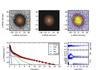 |
Fig. 4 BUDDA test: synthetic galaxy produced with Budda Bmod (see Sect. 3.2) and its Budda model in analogy to Fig. 2. |
The components were fitted with generalized ellipses 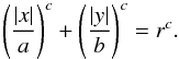 (4)A fixed parameter c = 2 corresponds to simple ellipses. This setup was used for the bulges and disks for which the code only fitted the ellipticity and the position angle. For a bar, the parameter was let free, mostly resulting in c > 2, that is, boxy ellipses.
The AGN was modeled using a circular Moffat distribution with FWHM fixed as the same as the PSF. The latter was measured in the image and kept fixed. Only the peak intensity of the AGN was fitted as a free parameter.
The results of the decomposition in the J-, H-, and K-band are presented in Tables 2−4. They give the structural parameters of bulge and disk as well as the luminosity fractions of the components. Figures with images of all decomposed galaxies and radial profiles are provided in the online version of this work (Fig. 15). Figure 2 shows an example of the surface-brightness fit for galaxy HE 2211–3903: the original image, the Budda model image and a residual image, obtained by dividing the galaxy image by the the model. Additionally, Fig. 2 shows the radial profile of the surface brightness of the galaxy, together with profiles of the individual components and the total model, as well as radial plots of the difference between the surface brightness of the galaxy and the model, ellipticity and position angle. All radial plots are based on ellipse fits with the Ellipse task of Iraf.
The residual images and radial profiles were used to check the quality of the models obtained with Budda. Furthermore, they can be used to identify otherwise hidden substructures and irregularities such as spiral arms (e.g. HE1310–1051), inner rings (e.g. HE2211–3903) or dust lanes (HE2204–3249). McLeod & Rieke (1995) considered a galaxy to have a bar if the ellipticity has a bump while the position angle stays constant and there is a shoulder in the intensity profile at the same position. We identify this behavior for instance in HE2211–3903. However, these authors reported that there are also galaxies that clearly show a bar in images but do not show these features in the radial profiles.
3.2. Reliability of Budda fits
We used Budda to fit the described brightness profiles (see Sect. 3.1) to the galaxy images. As results we obtained the structural parameters and images of the model components. From these data, we calculated the luminosities of the components. We are mainly interested in two parameters:
-
the flux of the host galaxy to estimate NIR colors(Sect. 3.3) and the stellar mass(Sect. 4.2);
-
the flux of the bulge component (equal to the host galaxy flux in case of elliptical galaxies) to estimate the black hole mass and/or study the black hole/bulge relationship.
To do this, we need to assess how well Budda reproduces these parameters. Therefore, we created artificial galaxy images with the Bmod (build model)-function of Budda. In particular, we produced 99 galaxies with bulge and AGN (displayed with circles in Fig. 3), 99 galaxies with bulge, disk, and AGN component (displayed with squares), and 99 galaxies with bulge, disk, bar, and AGN (displayed with diamonds). To produce the artificial galaxies, we assumed the profiles described in Sect. 3.1. Although the bar structure seems to be much more complex (e.g. Graham et al. 2011), in a first approach, we simulated bars by using a Sérsic profile with n ≈ 0.5...1. In all images, we added Gaussian noise. Then, we fitted the synthetic images with Budda, analogously to the science data. Figure 4 shows an example of an artificial barred galaxy and the Budda fit results.
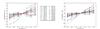 |
Fig. 5 Influence of the sky-background subtraction on the Budda fit in the K-band: we added a sky offset of (−3, −2, −1,1,2,3) × σsky to the sky subtracted images and repeated the fit. A positive sky offset means that the sky background was underestimated and therefore not completely subtracted. The plots show the hereby introduced deviation of the bulge (left) and host (right) magnitude. Positive magnitudes indicate an overestimation of the bulge/host, while negative magnitudes indicate an underestimation. |
Figure 3 (left) shows the deviation between host galaxy magnitude in the artificial image and the Budda fit as a function of the (fitted) AGN fraction. The quality of the fit is better for low AGN fractions. For AGN fractions below 30%, which is a good assumption in most cases, the difference is below 0.2 mag, which is acceptable. In cases of higher AGN fractions, the residuum should be analyzed carefully. We note that even in these cases the error in the measured properties of the AGN can be as low as 5%, and this feature arises because of the extraordinary brightness of the AGN. In inactive galaxies, this feature is absent, as previous tests have shown (de Souza et al. 2004; Gadotti 2009). We also investigated the quality of the bulge fits. Figure 3 (right) shows the deviation between bulge magnitude in the artificial image and the Budda fit as a function of the (fitted) bulge fraction. The difference in the bulge magnitude becomes lower with increasing bulge fraction. It is below 0.2 mag in most cases. Often, the fit is even better. In general, Budda tends to slightly overestimate (≈0.1 mag) the bulge component.
Since an accurate sky-background subtraction can be crucial for the reliability of the decomposition, especially in the NIR, we measured the sky background very thoroughly: following the practice of Vika et al. (2012), we measured the sky background by manually placing some fifty 10 × 10 pixel boxes around the galaxy and calculating the median value in each of these boxes. We then took the mean of these values as sky background and the standard deviation as measure of the spatial variability of the sky σsky. In general the sky background is close to zero, that is, it has been subtracted very well in the reduction process. However, if the measured sky background was not zero, as was the case in some images, we subtracted it subsequently. A background gradient was not observed in either case.
To estimate the influence of the background subtraction on the decomposition, we added sky offsets to the images ((−3, −2, −1,1,2,3) × σsky) and fitted them again. Figure 5 shows the difference in the bulge (left) and host (right) mangnitude compared with the fit without sky offset, exemplarily in K-band. In general, an underestimation of the sky background (resulting in a positive offset in the background-subtracted image) leads to an overestimation of the bulge and host flux and vice versa. However, in most cases the error is below the assumed errors introduced by calibration and decomposition. But in cases with low S/N (e.g., gal 70), the introduced errors can be large and an accurate sky subtraction is important.
3.3. Photometry
Near-infrared colors provide information on extinction and can help to distinguish whether the nuclear or the stellar component dominates the luminosity of the galaxy. Several components contribute to the NIR flux of an active galaxy and determine the colors: a stellar component, a non-stellar continuum source, an extinction component, and a component corresponding to the hot dust emission of the obscuring torus. Hyland & Allen (1982) calculated the colors of a zero-redshift quasar (i.e. an object entirely dominated by the nonstellar continuum emission instead of stellar emission) to be J − H = 0.95, H − K = 1.15. The colors of ordinary galaxies are J − H = 0.78, H − K = 0.22 (Glass 1984).
We measured the flux of the galaxies in three apertures after smoothing the images in the J-, H-, and K-band to a common seeing. We began with an aperture whose radius corresponded to the seeing FWHM and therefore mainly contained the nucleus. The second aperture has a radius of 4”. The third given value corresponds to the magnitude of the Budda model and was supposed to contain the complete object. All apertures were centered on the nucleus.
We also measured the NIR colors of the host galaxy. We used the Budda model of the stellar components. Spiral arms and other residual structures that are not modeled with Budda do not significantly affect our measurements. Gadotti (2008) pointed out that averaged over the complete annuli the deviation is almost zero. Therefore, we cannot deliver spatially resolved color information with our models. However, as we showed in Sect. 3.2, total fluxes are reliable. Therefore, the colors for the whole galaxy are expected to be reliable as well.
As expected from former studies (e.g. Fischer et al. 2006), the measured colors lie well between the positions of inactive galaxies and zero redshift quasars that can be seen in the color−color diagram in Fig. 6. Small apertures centered on the nucleus are redder than large apertures that contain the whole galaxy, including blue light from the host galaxy. However, some galaxies show an unexpected behavior, that is, the color of the nucleus is bluer than the color of the complete galaxy. These peculiarities coincide with irregularities in the decomposition (e.g. galaxy 82 or 89). The mean colors of the AGN-subtracted galaxies are J − H = 0.68 and H − K = 0.40. If we neglect galaxies with the above-mentioned irregularities and poor S/N, we obtain J − H = 0.73 and H − K = 0.35.
Until now, K-corrections have not been applied because they are strongly dependent on the shape of the SEDs, which are not known in our case. If we assume a typical stellar population of quiescent galaxies and use the corrections given by Fioc & Rocca-Volmerange (1999), KJ − H = −0.2z and KH − K = 2.7z, we obtain mean host galaxy colors of J − H = 0.74 and H − K = 0.25. The standard deviations of the sample are below σ = 0.15 in all cases. However, the measurement uncertainties are much higher. Taking into account decomposition (see Sect. 3.2) and calibration (see Sect. 2) errors, the uncertainties are around 0.2 mag. Taking into account these uncertainties, the colors are consistent with host galaxy colors in the literature, supporting the assumption that quasar host galaxies are not much different from “normal”, inactive galaxies.
We also measured the colors of only the AGN component model. The median colors are J − H = 0.92 and H − K = 0.80, which overlaps with the colors of the zero-redshift quasar. However, in this case, the standard deviations (σJ − H = 0.30 and σH − K = 0.66) as well as the measurement uncertainties are much higher.
NIR colors of the observed galaxies.
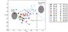 |
Fig. 6 NIR two-color diagram of the 20 observed galaxies. The sizes of data points symbols indicate the different apertures (small: 14″, medium: 8″, and large: 1.6″ diameter). The error bars in the lower right corner indicate the typical error for individual measurements. The expected locations of normal (i.e. inactive) galaxies and zero-redshift quasars are indicated by ellipses. |
3.4. Notes on individual objects
05 HE0036-5133
The galaxy is an elongated elliptical (ϵ = 0.4). The position in the color−color-diagram is consistent with a high AGN fraction. Only fits with AGN and one Sérsic-component are successful. However, the low resulting Sérsic-index of about 2, the bump in the ellipticity and the residuum can be seen as indicators for a hidden substructure. Fischer (2008) reported indications for a nuclear bar and spiral arms. These features cannot be seen with our resolution, but could be consistent with our results. A more detailed study is needed.
08 HE0045-2145
Almost face-on spiral galaxy with a bar and a disk scale-length of 3.3 kpc. There is possibly an inner ring that can only be seen in the residuum. The nuclear colors are bluer than the colors of the complete galaxy. Additionally, the fitted AGN fraction is very low. Optical spectra of this source (in preparation) suggest that the classification as Seyfert 1 is incorrect.
11 HE0103-5842
At first sight a barred galaxy. More precise inspection reveals a spiral structure inside the bar-like feature. This could be interpreted as a highly inclined spiral structure. In the residuum, a smaller-scaled elongated structure can be seen (possibly a bar?). Furthermore, additional large-scale structure − first interpreted as spiral arms − is seen. Its nature is unclear. Therefore, we classified the galaxy as irregular. A detailed study of the dynamics could be interesting.
16 HE0119-0118
The galaxy has a redshift of almost 0.06 and thus a small angular diameter. A very prominent bar and spiral arms make a good disk-fit impossible. In the residuum, indications for an inner ring can be seen. A bulge component could not be fitted. Therefore, we excluded this galaxy when estimating BH masses from the bulge luminosity.
24 HE0224-2834
This galaxy − the object with the highest redshift in our sample − is currently merging and highly perturbed. Because of the strong perturbations we only fit a general Sérsic-profile, resulting in a Sérsic index of n ≈ 4.5 and an effective radius of re = 4.4 kpc.
29 HE0253-1641
A face-on barred spiral galaxy. The bulge component is very compact with an effective radius of re = 0.8 kpc.
69 HE1248-1356
A highly inclined (i ≈ 69°) spiral galaxy at low redshift of z = 0.0145. The disk has a scale length of hr = 2.5 kpc and very prominent spiral arms. We see no indication for a substructure. However, because of the high inclination, the detection of a bar would be difficult. The AGN fraction is very low.
70 HE1256-1805
A circular elliptical. The galaxy is quite dim and a bright foreground star was in the field of view, resulting in a poor S/N. The nuclear colors indicate a low AGN fraction. This is consistent with the decomposition result (AGN fraction below 20%). The colors in larger apertures have large errors and thus are less reliable. The decomposition does not reveal any irregularities. We fit a Sérsic profile, resulting in an effective radius of re = 1.7 kpc and a Sérsic index of n ≈ 2 − 3.
71 HE1310-1051
The galaxy has no prominent features that deviate from the spherical symmetry in our NIR images. We fit an AGN component and a bulge component with effective radius re = 2.6 kpc and Sérsic index varying between n = 2.5 in the J-band and n = 4.3 in the K-band. The subtraction of the model reveals an arm-like structure that could be identified as spiral arms or tidal tails. In HST images (Malkan et al. 1998, as PG 1310-108), the arm is more prominent.
74 HE1330-1013
The galaxy has a disk scale length of hr = 8 kpc and shows a prominent elongated bar-like structure surrounded by a ring. On one side, a tail can be seen. Its origin cannot be explained with imaging data. A more detailed study to reveal the dynamical properties would be interesting. The bulge component has a low Sérsic-index value and lies slightly offset from the Kormendy-relation (Fig. 9). This could be seen as indication of a pseudo-bulge (Gadotti 2009).
75 HE1338-1423
The galaxy consists of a disk with an inclination i ≈ 54° and a scale length of hr = 9.6 kpc. Additionally, we found a spheroidal component with ellipticity ϵ ≈ 0.2 and effective radius 3.1 kpc, that is, we found a slightly smaller bulge and disk than in the fit of Jahnke et al. (2004). This could be an effect of including a bar in our fit. However, we found deviations from a purely elliptical shape, which might be indicative of a more complex structure, for instance, a warped disk.
77 HE1348-1758
A very circular elliptical. There are no signs for irregularities or perturbations. No candidates for companion galaxies are found in the field of view.
79 HE1417-0909
In the K-band image, we were unable to avoid residua originating from the data reduction. Therefore, the colors and fits are not reliable. We found an elliptical with ϵ = 0.4 and no other irregularities. There are several neighboring galaxies at the same redshift in the region (distance ≈0.5−1′, redshift from NED), which could be interacting with HE1417–0909. Another cluster of galaxies at the same redshift can be found at ≈6′ distance.
80 HE2112-5926
A very circular elliptical with no sign for perturbations. The center as well as the AGN-subtracted host galaxy are very red. However, the decomposition reveals a low AGN fraction. The reddening is more likely to come from dust extinction. There is a nearby companion (spiral galaxy), which forms the interacting galaxy pair ESO 144-IG 021 with HE2112–5926.
81 HE2128-0221
A very elongated elliptical with ϵ = 0.5 at a redshift of z = 0.0528. We fit a Sérsic profile with re = 2 kpc and n ≈ 3. The residuum implies a substructure. However, we were unable to find indications of other structures, neither in optical, nor in SDSS images.
82 HE2129-3356
We found an elongated elliptical. The color analysis shows that the host is redder than the nucleus. Decomposition indicates that the AGN fraction is very low and even drops in the K-band. We found the galaxy to be surrounded by several objects, some of them extended. However, we have no additional information about these objects and cannot confirm interaction.
83 HE2204-3249
The AGN fraction in the H-band is lower than expected compared with that of the J- and K-band. Additionally, the host galaxy is redder than the nucleus. We suspect that a dust lane follows the semi-major axis of the galaxy. This is supported by the residual image of our decomposition analysis, which clearly indicates a residual structure that follows the symmetry axis of the galaxy.
84 HE2211-3903
A spiral galaxy with a disk scale-length of hr = 5 kpc and a small bulge (re = 1.4 kpc). The 2D decomposition of this barred spiral galaxy reveals an inner ring and a third spiral arm (see also Scharwächter et al. 2011).
85 HE2221-0221
Very symmetric, almost circular elliptical with re = 2.4 kpc. The nuclear colors are very red. This is consistent with the high AGN fraction of 65% obtained from our fits in K-band.
89 HE2236-3621
The decomposition of this quite dim elliptical galaxy reveals a tail-like irregularity. The residuum also shows an irregularity in the center (which cannot be explained by a PSF-mismatch, etc.). The origin of the perturbation is unclear.
4. Discussion
We discuss the results of photometry and decomposition by commenting on the morphology, estimating stellar and black hole masses, and bringing them into context with the overall AGN population.
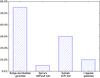 |
Fig. 7 Distribution of Hubble types of the 20 observed galaxies. |
4.1. Morphology
Of the 20 observed objects, we classified eleven as bulge dominated. In one case, we fitted only disk and bar. Eight galaxies have disk and bulge components. Seven galaxies show a prominent bar. Figure 7 shows a histogram of the Hubble classification of the 20 galaxies that are examined in this study.
In this paper, we present a detailed study of the structural parameters based on decomposition. In a previous study (Busch et al. 2013), however, we presented a morphological classification that was only based on visual inspection. We used images of an additional 26 galaxies from the SDSS (optical) and the ESO archive (NIR, obtained with NACO and ISAAC) to augment our morphological statistics. This resulted in 46 galaxies, almost 50% of the LLQSO sample. The statistics show consistently that the fraction of barred galaxies within spiral galaxies is very high (6 out of 7, resp. 19 out of 22 (86%) spiral galaxies are barred). Observations of the remaining 53 galaxies of the LLQSO sample might be useful to ensure the statistical significance.
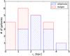 |
Fig. 8 Histograms of the effective radius of the bulge component (red) of spiral galaxies or the whole host galaxy for elliptical galaxies (blue). To calculate the physical scales, we assumed the standard cosmology described in Sect. 1. |
Lee et al. (2012b) analyzed a volume-limited sample of SDSS galaxies with 0.01 < z < 0.05, Mr < − 20.3 and M∗ > 1010 M⊙, similar to our sample. They found a bar-fraction of 41.4% at optical wavelengths. Other studies (e.g. Hao et al. 2009; Lee et al. 2012a) likewise suggested that one third of the spiral galaxies is barred at optical wavelengths. However, in the NIR, the bar detection rate tends to be higher, about two thirds (Kormendy & Kennicutt 2004). The bar fraction in the sample presented here is higher. This is an interesting fact since bars are commonly seen as a possible way to fuel central SMBHs (e.g. Combes 2003). On the other hand, it is discussed that bars are not the only way to feed the central engine. Some groups have observed a higher bar fraction in AGN galaxies than in non-AGN galaxies (e.g. Laine et al. 2002). However, Lee et al. (2012b) found that no significant difference in bar fraction between active and inactive galaxies can be observed if one compares samples of galaxies that are matched in mass, color, etc.
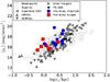 |
Fig. 9 Comparison of the observed LLQSOs with data from other studies in a plot of mean surface brightness within the effective radius ⟨ μe ⟩ vs. effective radius re(in kpc), as presented in Dasyra et al. (2007). This plot is a projection of the fundamental plane of early-type galaxies, often called Kormendy relation. |
The distribution of the linear extent of the central spheroidal components is shown in Fig. 8. Disk scale-lengths range from 2.5 to 9.6 kpc, with an average of 5 kpc. The effective radii of the spheroidal component of the spiral galaxies range from 0.5 to 3.0 kpc, with an average of 1.3 kpc. The effective radii of the elliptical hosts range from 1.2 to 4.5 kpc, with an average of 2.7 kpc. Dasyra et al. (2007) observed 12 local (mainly Palomar-Green) QSOs and found a mean effective radius of 3.9 kpc for QSOs and 2.2 kpc for ULIRGs, analyzed in previous studies (Dasyra et al. 2006a,b). Jahnke et al. (2004) observed nearby quasars compiled from the Hamburg/ESO survey and found a mean effective radius of 5.4 kpc for the elliptical hosts. In this sample with even closer galaxies (z < 0.06), we found a mean effective radius of 2.7 kpc for elliptical galaxies of the sample. We conclude that the LLQSOs are less extended than the more powerful PG quasars and HES quasars.
To investigate the dynamical properties of the spheroids of the host galaxies in more detail, we investigated the positions of the objects in the fundamental plane (Djorgovski & Davis 1987; Dressler et al. 1987). Kinematics and light distribution are both consequences of the overall dynamical state of the system. Furthermore, the light distribution depends on the mass-to-light ratio M∗/L and thus on the star formation history. Massive elliptical galaxies and classical bulges follow a well-defined relation in the Reff − μeff projection of the fundamental plane using the effective radius reff and the mean K-band surface brightness within the effective radius ⟨ μeff ⟩ from the Budda fits. This relation is also known as the Kormendy-relation (first published by Kormendy 1977). Pseudo-bulges that are built by secular evolution and therefore show different dynamics, are supposed to be found as outliers of this relation (Gadotti 2009).
In Fig. 9, we show our data points (blue circles for elliptical galaxies, red squares for bulges of spiral galaxies) together with data points for cluster-, moderate-, and giant ellipticals, luminous infrared galaxies (LIRGs), ultraluminous infrared galaxies (ULIRGs), other merger remnants, giant host QSOs and PG QSOs, collected by Dasyra et al. (2007). In this diagram, the data points of the observed galaxies lie in the region of classically built (i.e. by mergers) bulges and ellipticals and therefore do not show clear evidence for the dominance of secular processes.
4.2. Stellar masses
When photometric measurements of the host galaxies are available, estimates of the
stellar mass can be made using the mass-to-light ratio
M∗/L. Our 2D decompositions result in
models for the different components. We considered all components, except the AGN
component, to calculate the luminosity of the host galaxy. Zibetti et al. (2009) expressed the
M∗/L ratio in the H-band
as a function of the two colors (g − i) and
(i − H) with a typical accuracy of 30 per cent. Bell et al. (2003) also used SDSS and 2MASS to calculate
galaxy luminosity and stellar mass functions in the local Universe. They found a relation
between M/L ratio in the NIR and optical
(B − V) colors with the general form 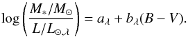 (5)The constants are
aJ = −0.261,aH = −0.209,aK = −0.206,bJ = 0.433,bH = 0.210,
and bK = 0.135. The authors adopted a “diet”
Salpeter initial mass function (IMF). In case of a Kroupa IMF, for example, the zero
points aλ have to be modified by subtracting
0.15 dex.
(5)The constants are
aJ = −0.261,aH = −0.209,aK = −0.206,bJ = 0.433,bH = 0.210,
and bK = 0.135. The authors adopted a “diet”
Salpeter initial mass function (IMF). In case of a Kroupa IMF, for example, the zero
points aλ have to be modified by subtracting
0.15 dex.
Host luminosities and stellar masses.
Because of the absence of measured optical colors, we decided to apply Eq. (5) and used average colors of (B − V) = 0.9 and (B − V) = 0.7 for inactive elliptical/S0 galaxies and spiral galaxies resp. (Fukugita et al. 1995). As we discuss in the following subsection, the M∗/L ratio of type-1 AGN hosts is unknown (Schawinski et al. (2010) found that hosts of narrow-line AGNs lie in the “green valley”, while Trump et al. (2013) reported that more luminous broad-line AGN have bluer host galaxies.). Assuming that typical galaxy colors range between (B − V) = 0.5−1.0, we found that the M∗/L-ratio ranges between 0.90−1.49 for the J-band, 0.79−1.00 for the H-band, and 0.73−0.85 for the K-band. The color-dependence of the M∗/L ratio in the K-band is the weakest. However, as the AGN fraction grows in the K-band, the uncertainty introduced by the AGN subtraction typically becomes larger.
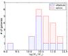 |
Fig. 10 Histogram of the stellar masses of the galaxies. The different colors indicate the morphology of the host galaxy. |
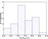 |
Fig. 11 Histogram of the SMBH masses in the low-luminosity type-1 QSO sample. BH masses of 74 galaxies have been measured. |
Table 6 shows the results of our calculations. The mass estimates calculated from the three different bands are consistent despite the uncertainties mentioned. In Fig. 10, we show a histogram of the stellar masses (averages of the mass estimates from the three bands) with different colors indicating the host galaxy’s morphology. We found the average mass to be 6.7 × 10¹⁰ M⊙. Baldry et al. (2008) found a stellar mass function in the local Universe with M∗ = 4.6 × 10¹⁰ M⊙. However, they assumed a Chabrier IMF (Chabrier 2003). Converting this to the IMF assumed in our calculations, we obtained M∗ ≈ 6 − 8 × 10¹⁰ M⊙, that is, the observed LLQSOs have stellar masses on the order of ~ M∗.
Dasyra et al. (2007) found the stellar masses of the spheroids to be 2.1 × 10¹¹ M⊙ on average, which corresponds to ~ 3 M∗ (or ~ 1.5 M∗ in their choice of M∗). We conclude that the hosts of our LLQSOs are on average less massive than PG quasars and therefore have stellar masses between local galaxies and PG quasars.
Bulge magnitudes and black hole masses.
4.3. Black hole masses
For 74 galaxies from the LLQSO sample, eleven of which are analyzed in this paper, black hole masses are available from Schulze et al. (2009), Schulze & Wisotzki (2010), and Schulze (priv. comm.). In several observation campaigns, they took optical spectra of most of the type-1 AGN in the HES and computed BH masses using the scaling relation between broad line region (BLR) size and continuum luminosity by Bentz et al. (2009) and the scale factor f = 3.85 from Collin et al. (2006), 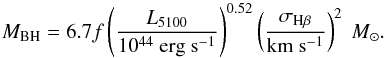 (6)Depending on the choice of slope and scale factor f, virial BH-mass estimators can differ by about 0.38 dex (McGill et al. 2008). Particularly, using a more recent scale factor for active galaxies f = 5.9 (Woo et al. 2013) shifts the BH masses up by ΔMBH = 0.19 dex. In Fig. 11, we show a histogram of the measured BH masses. In the LLQSO sample, they range from 6.0 < log (MBH/M⊙) < 8.7 with a median of log (MBH/M⊙) = 7.4. Dasyra et al. (2007) found the BH masses to be typically around 108 M⊙. We conclude that the observed LLQSOs have less massive central black holes than PG quasars. Greene & Ho (2006) compiled a sample of 88 spectroscopically identified AGN with z ≤ 0.05. The BH masses typically range from 5.0 < log (MBH/M⊙) < 8.5 with log (MBH/M⊙) = 7.0. This is consistent with our findings. Bennert et al. (2011) observed type-1 AGN in a similar redshift range but selected only galaxies with MBH > 107 M⊙. However, also in this study, only a few (2/25) galaxies with MBH > 108 M⊙ were found. Panessa et al. (2006) analyzed 60 Seyfert galaxies from the Palomar optical spectroscpic survey of nearby galaxies (39 type-2, 13 type-1, 8 at boundary between Seyferts and LINERs or H ii-region classification). Their BH masses range from 4.9 < log (MBH/M⊙) < 8.8 with a median of log (MBH/M⊙) = 7.6 (median mass log (MBH/M⊙) = 7.3 for type-1 only) which is similar to our slightly more distant objects.
In the past decade, tight connections between black hole masses and properties of the central spheroidal component have been found. With high-quality near-infrared imaging data at hand, we used the MBH − Lbulge relation that connects black hole mass and NIR luminosity of the bulge component. Marconi & Hunt (2003) first found a correlation ![Mathematical equation: \begin{equation} \log \left( \frac{M_\mathrm{BH}}{M_\odot} \right) = a_\lambda + b_\lambda \cdot \left[ \log \left( \frac{L_{\mathrm{bul},\lambda}}{L_{\odot,\lambda}} \right) - c_\lambda \right] , \end{equation}](/articles/aa/full_html/2014/01/aa22486-13/aa22486-13-eq222.png) (7)which, for the BH mass range of their sample, has a scatter similar to that of the MBH − σ relation. The constants for the three bands used in this study are aJ = 8.10,aH = 8.04,aK = 8.08, bJ = 1.24,bH = 1.25,bK = 1.21,cJ = 10.7,cH = 10.8, and cK = 10.9.
(7)which, for the BH mass range of their sample, has a scatter similar to that of the MBH − σ relation. The constants for the three bands used in this study are aJ = 8.10,aH = 8.04,aK = 8.08, bJ = 1.24,bH = 1.25,bK = 1.21,cJ = 10.7,cH = 10.8, and cK = 10.9.
The BH masses and bulge magnitudes derived for the LLQSOs in this paper are listed in Table 7. We have corrected the magnitudes for the systematic effect seen in Sect. 3.2. To do this, we determined the mean deviation of the fitted bulge magnitude in bins of 20% in the bulge fraction and subtracted this value from the measured value. The corrections are lower than 0.15 mag. In Fig. 12, we plot our data points together with a simple regression line and published MBH − Lbulge relations by Marconi & Hunt (2003), Vika et al. (2012), and Graham & Scott (2013). As error of the bulge magnitudes, we adopted the scatter we measured in the corresponding bulge-fraction bin in Sect. 3.2 (Fig. 3 right). The errors of the black hole masses are assumed to be 0.3 dex. Our data points follow none of these relations. In Fig. 14 we plot the black hole masses of the galaxies of this study as function of the absolute K-band magnitude together with data points collected in previous studies. We clearly see that the LLQSOs observed in this study lie below the location of the inactive classical bulges and ellipticals.
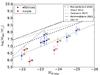 |
Fig. 12 Correlation between black hole mass MBH and absolute K-band magnitude MK of the bulge or the elliptical galaxy. Our data (red squares indicate disk-dominated galaxies, blue circles bulge-dominated galaxies) plotted together with the MBH − Lbulge relations of Marconi & Hunt (2003), Vika et al. (2012), Graham & Scott (2013), and Kormendy & Ho (2013). Our best fit is shown as the solid green line for comparison. |
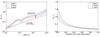 |
Fig. 13 Left: M∗/Lλ ratio in J-, H-, and K-bands of the young stellar population as a function of age. Different colors indicate the three bands. The solid line shows an instantaneous star burst, the dashed line plots continuous star formation (1 M⊙ yr-1). Right: M∗/Lλ ratio as function of the mass fraction of a 0.1 Gyr population added to an old (10 Gyr) population. |
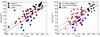 |
Fig. 14 Correlation between black hole mass MBH and absolute K-band magnitude MK of the bulge or the elliptical galaxy. Left: LLQSOs (blue squares) together with data collected by Kormendy & Ho (2013). Right: LLQSOs together with data collected by Graham & Scott (2013). The lines indicate the same relations as in Fig. 12. |
Basically, we can consider two explanations of this discrepancy: (a) the bulges are overluminous and/or (b) the black holes are undermassive. In Sect. 3.2, we show that the decomposition with Budda causes errors. However, the results of our tests indicate that the bulge-brightness fit uncertainties (a few tenths of dex in luminosity) are not large enough to explain our finding. Schulze et al. (2009) reported that they did not correct their continuum luminosities L5100 for the host galaxy contribution. However, this effect is expected to be weak and more importantly shift the black hole masses to even lower masses. Thus, the deviation of the observed LLQSOs from the MBH − Lbulge relations of inactive galaxies is too high to be explained by the expected measurement uncertainties.
An offset of type-1 AGN from the (optical) MBH − Lbulge relation has been reported by Nelson et al. (2004) and Kim et al. (2008). In a pilot study, Bennert et al. (2011) connected SDSS images and high-quality Keck/LIRS long-slit spectra of nearby type-1 AGNs to study the relations between central black holes and host galaxies. While they found that the MBH − M∗ and MBH − σ relation of active galaxies agrees with those of inactive ones, they also found an offset in the MBH − Lbulge relation (in V-band) and reported the host galaxies to be overluminous by 0.4 mag on average. Nelson et al. (2004) suggested that brighter bulges can be explained by lower M/L ratios. They used Guy Worthey’s Dial-a-Galaxy Website (Worthey 1994) to show that the mixing of 15% 1 Gyr and 85% 12 Gyr population results in a ≈0.5 mag brighter bulge than a bulge with old populations only.
The so-called narrow-line Seyfert-1s (NLS1s) are galaxies with relatively small black holes and high Eddington ratios, indicating a strong black hole growth (e.g., Boroson 2011). The observed objects have a mean Eddington ratio3 of ηav = 0.18 (median ηmedian = 0.082), indicating efficient accretion but not conspicuously heavily growing black holes as seen in some NLS1s. It has been found that NLS1s also lie below the MBH − Lbulge relation of inactive galaxies (Wandel 2002; Ryan et al. 2007), while they seem to follow the MBH − σ∗ relation (Komossa & Xu 2007). Since NLS1s might be the low-MBH tail (see discussion in Valencia-S. et al. 2013) of the type-1 AGN population, we expect them to show the same trend as our sample of type-1 sources.
Model calculations show that the ratio of stellar mass and K-band luminosity, M∗/LK, is a good estimator for the age of stellar populations because it increases monotonically with time. In practice, old and young stellar populations cannot easily be separated. However, the overall M∗/LK ratio can be used as an upper limit of the age of the young stellar population (see discussion in Davies et al. 2007). We used starburst99 (Leitherer et al. 1999; Vázquez & Leitherer 2005) to estimate the M∗/Lλ ratio for the J, H and K band as a function of the age of the stellar population (Fig. 13 left). In Fig. 13 (right), we show the M∗/Lλ ratio that results when one mixes a 0.1 Gyr population with an old 10 Gyr population. The M∗/Lλ ratio decreases monotonically with increasing fraction of the intermediate-age population.
Given that former studies (Bennert et al. 2011) indicated that active galaxies follow the same MBH − M∗ relation as inactive ellipticals, we calculated the M∗/Lλ ratios that would be necessary to shift the observed galaxies on the MBH − M∗ relation  (8)of inactive galaxies (Häring & Rix 2004). With the M∗/Lλ ratios presented in Table 7, we can now estimate the amount of intermediate-age stellar populations that have to be added to an old population to reproduce the observed M∗/Lλ ratio. With the exception of galaxy 82, none of the galaxies would only contain old stellar populations. Instead, the galaxies should contain a considerable amount of intermediate-age stellar populations (e.g. Jahnke et al. 2004). Under the assumption that these galaxies follow the MBH − M∗ relation of inactive galaxies, at least four or five galaxies (08, 11, 75, 77, and probably 24) would be dominated by a young 0.1 Gyr population, in contrast to the traditional view of bulge composition.
Discarding the assumption that active galaxies follow the same MBH − M∗ relation as inactive galaxies, an alternative interpretation is that undermassive black holes are hosted in normal bulges. At the current accretion rate, the systems would require one typical AGN duty cycle (without additional star formation) to reach the MBH − Lbulge relation of inactive galaxies.
Recently, a bent MBH − Lbulge relation has been suggested (Graham 2012; Graham & Scott 2013). This relation has different slopes for core-Sérsic galaxies (Graham et al. 2003) and Sérsic galaxies that are thought to originate from different building mechanisms (dry merging vs. gaseous formation processes). The scatter of the relation for Sérsic galaxies that show a trend for lower MBH is higher than that of the single power-law relations. In our study, we cannot distinguish between core-Sérsic and Sérsic galaxies because of the AGN subtraction and the lower resolution (owing to the higher distances of the observed LLQSOs). We note that several galaxies that are classified as Sérsic galaxies by Graham & Scott (2013) are classified as hosts of pseudo-bulges by Kormendy & Ho (2013) and have therefore been excluded from the MBH − Lbulge relation fit of the latter.
When comparing the observed LLQSOs with the bent relation by Graham & Scott (2013), more than half of the observed galaxies would lie within the scatter of the relation (see Fig. 14). However, the trend that they are significantly below the predicted relation remains and has to be investigated in more detail.
We are carrying out further studies with multiwavelength spectroscopic techniques to gain deeper insights into the circumnuclear star-forming properties of the observed galaxies and specify the amount of star formation in LLQSOs.
5. Summary and conclusions
The low-luminosity type-1 QSO sample is suitable for detailed spatially resolved studies of nearby QSOs. We investigated 20 galaxies with high-quality NIR imaging data. The results of our analysis can be summarized as follows:
-
1.
We presented the morphological classification and supportedthe statistics with additional data that we inspected by eye only.We found that 86% of the spiral galaxies are barred and many ofthem have other peculiarities such as inner rings.
-
2.
We measured NIR colors in different apertures and found that the galaxies are broadly distributed across the whole range between inactive galaxies and zero-redshift quasars. The colors of the AGN-subtracted galaxies are consistent with previous studies.
-
3.
We found Budda to be suitable and reliable for decompositions of nearby active galaxies. The limits of this method have been probed in Sect. 3.2. We used Budda to extract single components or subtract the AGN component to investigate host galaxy properties.
-
4.
From the models obtained by decomposition with Budda we estimated stellar masses that range from 2 × 10⁹ M⊙ to 2 × 10¹¹ M⊙ with an average mass of 7 × 10¹⁰ M⊙ by applying a typical mass-to-light ratio.
-
5.
In comparison with other samples that contain more luminous QSOs, we found our galaxies to have lower stellar and black hole masses. They are less luminous, considering both nuclear and host galaxy luminosity. In the fundamental plane, the observed LLQSOs lie between luminous QSOs and inactive local galaxies. Along with the findings of Bertram et al. (2007) and Moser et al. (2013), this implies that LLQSOs populate an intermediate region between nearby Seyfert galaxies, (ultra-)luminous infrared galaxies and luminous QSOs in terms of many parameters such as z, MBH, Lbol, Lhost, SFR.
-
6.
We found that the LLQSOs observed in this study do not follow the MBH − Lbulge relations for inactive galaxies. Previous studies at optical wavelengths have often explained this by star formation in the spheroids of active galaxies. An in-depth investigation of the amount of star formation in the observed sources in order to constrain the account of star formation in shifting active galaxies off the MBH − Lbulge relations is needed.
Online material
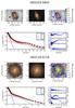 |
Fig. 15 continued. |
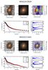 |
Fig. 15 continued. |
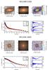 |
Fig. 15 continued. |
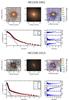 |
Fig. 15 continued. |
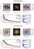 |
Fig. 15 continued. |
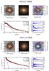 |
Fig. 15 continued. |
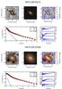 |
Fig. 15 continued. |
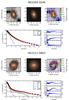 |
Fig. 15 continued. |
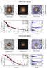 |
Fig. 15 continued. |
AGN with broad permitted lines in the optical spectra are referred to as “type-1”.
The Eddington ratio is a measure of the accretion efficiency and is defined as  (Elvis et al. 1994).
Acknowledgments
The authors kindly thank Andreas Schulze for providing black-hole mass estimates and emission-line characteristics of the LLQSOs. Furthermore, the authors thank the anonymous referee, Alister Graham, Dongchan Kim, and Davide Lena for comments that helped to improve the manuscript. G.B. is a member of the Bonn-Cologne Graduate School of Physics and Astronomy and acknowledges support from the Konrad-Adenauer-Stiftung. J.Z. acknowledges support from the European project EuroVO DCA under the Research e-Infrastructures area (RI031675). J.S., S.F. and J.Z. acknowledge support by the German Academic Exchange Service (DAAD) under project number 50753527. J.S. acknowledges the European Research Council’s Advanced Grant Program Num 267399-Momentum. M.V.-S. acknowledges funding from the European Union Seventh Framework Programme (FP7/2007-2013) under grant agreement No. 312789. We acknowledge fruitful discussions with members of the European Union funded COST Action MP0905: Black Holes in a violent Universe, and of the COST Action MP1104: Polarization as a tool to study the Solar System and beyond. Part of this work was supported by the German Deutsche Forschungsgemeinschaft, DFG project numbers SFB 494 and SFB 956. This work is supported in part by the German Federal Department for Education and Research (BMBF) under grants Verbundforschung 05AL5PKA/0 and 05A08PKA. Parts of the observations were conducted at the LBT Observatory, a joint facility of the Smithsonian Institution and the University of Arizona. LBT observations were obtained as part of the Rat Deutscher Sternwarten guaranteed time on Steward Observatory facilities through the LBTB coorperation. This research has made use of the NASA/IPAC Extragalactic Database (NED) which is operated by the Jet Propulsion Laboratory, California Institute of Technology, under contract with the National Aeronautics and Space Administration.
References
- Aird, J., Nandra, K., Laird, E. S., et al. 2010, MNRAS, 401, 2531 [NASA ADS] [CrossRef] [Google Scholar]
- Baldry, I. K., Glazebrook, K., & Driver, S. P. 2008, MNRAS, 388, 945 [NASA ADS] [Google Scholar]
- Bell, E. F., McIntosh, D. H., Katz, N., & Weinberg, M. D. 2003, ApJS, 149, 289 [NASA ADS] [CrossRef] [Google Scholar]
- Bennert, V. N., Auger, M. W., Treu, T., Woo, J.-H., & Malkan, M. A. 2011, ApJ, 726, 59 [NASA ADS] [CrossRef] [Google Scholar]
- Bentz, M. C., Peterson, B. M., Netzer, H., Pogge, R. W., & Vestergaard, M. 2009, ApJ, 697, 160 [Google Scholar]
- Bertram, T., Eckart, A., Fischer, S., et al. 2007, A&A, 470, 571 [NASA ADS] [CrossRef] [EDP Sciences] [Google Scholar]
- Boroson, T. A. 2011, in Narrow-Line Seyfert 1 Galaxies and their Place in the Universe, PoS, NLS1, 3 [Google Scholar]
- Busch, G., Zuther, J., Valencia-S., M., Moser, L., & Eckart, A. 2013, in Proc. Conf. Nuclei of Seyfert galaxies and QSOs − Central engine & conditions of star formation, PoS, in press [arXiv:1307.1049] [Google Scholar]
- Caon, N., Capaccioli, M., & D’Onofrio, M. 1993, MNRAS, 265, 1013 [NASA ADS] [CrossRef] [Google Scholar]
- Chabrier, G. 2003, PASP, 115, 763 [NASA ADS] [CrossRef] [Google Scholar]
- Collin, S., Kawaguchi, T., Peterson, B. M., & Vestergaard, M. 2006, A&A, 456, 75 [NASA ADS] [CrossRef] [EDP Sciences] [Google Scholar]
- Combes, F. 2003, in Active Galactic Nuclei: From Central Engine to Host Galaxy, eds. S. Collin, F. Combes, & I. Shlosman, ASP Conf. Ser., 290, 411 [Google Scholar]
- Dasyra, K. M., Tacconi, L. J., Davies, R. I., et al. 2006a, ApJ, 638, 745 [NASA ADS] [CrossRef] [Google Scholar]
- Dasyra, K. M., Tacconi, L. J., Davies, R. I., et al. 2006b, ApJ, 651, 835 [NASA ADS] [CrossRef] [Google Scholar]
- Dasyra, K. M., Tacconi, L. J., Davies, R. I., et al. 2007, ApJ, 657, 102 [NASA ADS] [CrossRef] [Google Scholar]
- Davies, R. I., Müller Sánchez, F., Genzel, R., et al. 2007, ApJ, 671, 1388 [NASA ADS] [CrossRef] [Google Scholar]
- de Souza, R. E., Gadotti, D. A., & dos Anjos, S. 2004, ApJS, 153, 411 [NASA ADS] [CrossRef] [Google Scholar]
- de Vaucouleurs, G. 1948, Ann. Astrophys., 11, 247 [Google Scholar]
- Djorgovski, S., & Davis, M. 1987, ApJ, 313, 59 [NASA ADS] [CrossRef] [Google Scholar]
- Dressler, A., Lynden-Bell, D., Burstein, D., et al. 1987, ApJ, 313, 42 [NASA ADS] [CrossRef] [Google Scholar]
- Elvis, M., Wilkes, B. J., McDowell, J. C., et al. 1994, ApJS, 95, 1 [NASA ADS] [CrossRef] [Google Scholar]
- Ferrarese, L., & Merritt, D. 2000, ApJ, 539, L9 [NASA ADS] [CrossRef] [Google Scholar]
- Fioc, M., & Rocca-Volmerange, B. 1999, A&A, 351, 869 [NASA ADS] [Google Scholar]
- Fischer, S. 2008, Ph.D. Thesis, University of Cologne, Germany [Google Scholar]
- Fischer, S., Iserlohe, C., Zuther, J., et al. 2006, A&A, 452, 827 [NASA ADS] [CrossRef] [EDP Sciences] [Google Scholar]
- Freeman, K. C. 1970, ApJ, 160, 811 [NASA ADS] [CrossRef] [Google Scholar]
- Fukugita, M., Shimasaku, K., & Ichikawa, T. 1995, PASP, 107, 945 [NASA ADS] [CrossRef] [Google Scholar]
- Gadotti, D. A. 2008, MNRAS, 384, 420 [NASA ADS] [CrossRef] [Google Scholar]
- Gadotti, D. A. 2009, MNRAS, 393, 1531 [NASA ADS] [CrossRef] [Google Scholar]
- Gaffney, N. I., Lester, D. F., & Doppmann, G. 1995, PASP, 107, 68 [NASA ADS] [CrossRef] [Google Scholar]
- Gebhardt, K., Bender, R., Bower, G., et al. 2000, ApJ, 539, L13 [NASA ADS] [CrossRef] [Google Scholar]
- Glass, I. S. 1984, MNRAS, 211, 461 [NASA ADS] [Google Scholar]
- Graham, A. W. 2012, ApJ, 746, 113 [NASA ADS] [CrossRef] [Google Scholar]
- Graham, A. W., & Driver, S. P. 2007, ApJ, 655, 77 [NASA ADS] [CrossRef] [Google Scholar]
- Graham, A. W., & Li, I.-H. 2009, ApJ, 698, 812 [NASA ADS] [CrossRef] [Google Scholar]
- Graham, A. W., & Scott, N. 2013, ApJ, 764, 151 [NASA ADS] [CrossRef] [Google Scholar]
- Graham, A. W., Erwin, P., Trujillo, I., & Asensio Ramos, A. 2003, AJ, 125, 2951 [NASA ADS] [CrossRef] [Google Scholar]
- Graham, A. W., Onken, C. A., Athanassoula, E., & Combes, F. 2011, MNRAS, 412, 2211 [NASA ADS] [CrossRef] [Google Scholar]
- Greene, J. E., & Ho, L. C. 2006, ApJ, 641, L21 [NASA ADS] [CrossRef] [Google Scholar]
- Hao, L., Jogee, S., Barazza, F. D., Marinova, I., & Shen, J. 2009, in Galaxy Evolution: Emerging Insights and Future Challenges, eds. S. Jogee, I. Marinova, L. Hao, & G. A. Blanc, ASP Conf. Ser., 419, 402 [Google Scholar]
- Häring, N., & Rix, H.-W. 2004, ApJ, 604, L89 [NASA ADS] [CrossRef] [Google Scholar]
- Heckman, T. M., Kauffmann, G., Brinchmann, J., et al. 2004, ApJ, 613, 109 [NASA ADS] [CrossRef] [Google Scholar]
- Ho, L. 1999, in Observational Evidence for the Black Holes in the Universe, ed. S. K. Chakrabarti, Astrophys. Space Sci. Lib., 234, 157 [Google Scholar]
- Hopkins, A. M., & Beacom, J. F. 2006, ApJ, 651, 142 [NASA ADS] [CrossRef] [MathSciNet] [Google Scholar]
- Hyland, A. R., & Allen, D. A. 1982, MNRAS, 199, 943 [NASA ADS] [CrossRef] [Google Scholar]
- Jahnke, K., Kuhlbrodt, B., & Wisotzki, L. 2004, MNRAS, 352, 399 [NASA ADS] [CrossRef] [Google Scholar]
- Kim, M., Ho, L. C., Peng, C. Y., et al. 2008, ApJ, 687, 767 [NASA ADS] [CrossRef] [Google Scholar]
- Komossa, S., & Xu, D. 2007, ApJ, 667, L33 [NASA ADS] [CrossRef] [Google Scholar]
- König, S., Eckart, A., García-Marín, M., & Huchtmeier, W. K. 2009, A&A, 507, 757 [NASA ADS] [CrossRef] [EDP Sciences] [Google Scholar]
- König, S., Eckart, A., Henkel, C., & García-Marín, M. 2012, MNRAS, 420, 2263 [NASA ADS] [CrossRef] [Google Scholar]
- Kormendy, J. 1977, ApJ, 218, 333 [NASA ADS] [CrossRef] [Google Scholar]
- Kormendy, J., & Ho, L. C. 2013, ARA&A, 51, 511 [Google Scholar]
- Kormendy, J., & Kennicutt, Jr., R. C. 2004, ARA&A, 42, 603 [NASA ADS] [CrossRef] [Google Scholar]
- Kormendy, J., & Richstone, D. 1995, ARA&A, 33, 581 [NASA ADS] [CrossRef] [Google Scholar]
- Kormendy, J., Bender, R., & Cornell, M. E. 2011, Nature, 469, 374 [NASA ADS] [CrossRef] [Google Scholar]
- Laine, S., Shlosman, I., Knapen, J. H., & Peletier, R. F. 2002, ApJ, 567, 97 [NASA ADS] [CrossRef] [Google Scholar]
- Lee, G.-H., Park, C., Lee, M. G., & Choi, Y.-Y. 2012a, ApJ, 745, 125 [NASA ADS] [CrossRef] [Google Scholar]
- Lee, G.-H., Woo, J.-H., Lee, M. G., et al. 2012b, ApJ, 750, 141 [NASA ADS] [CrossRef] [Google Scholar]
- Leitherer, C., Schaerer, D., Goldader, J. D., et al. 1999, ApJS, 123, 3 [NASA ADS] [CrossRef] [Google Scholar]
- Madau, P., Pozzetti, L., & Dickinson, M. 1998, ApJ, 498, 106 [NASA ADS] [CrossRef] [Google Scholar]
- Magorrian, J., Tremaine, S., Richstone, D., et al. 1998, AJ, 115, 2285 [NASA ADS] [CrossRef] [Google Scholar]
- Malkan, M. A., Gorjian, V., & Tam, R. 1998, ApJS, 117, 25 [NASA ADS] [CrossRef] [Google Scholar]
- Marconi, A., & Hunt, L. K. 2003, ApJ, 589, L21 [NASA ADS] [CrossRef] [Google Scholar]
- McGill, K. L., Woo, J.-H., Treu, T., & Malkan, M. A. 2008, ApJ, 673, 703 [NASA ADS] [CrossRef] [Google Scholar]
- McLeod, K. K. 1997, in Quasar Hosts, Proc. ESO-IAC Conf., eds. D. L. Clements, & I. Perez-Fournon (Berlin: Springer-Verlag), 45 [Google Scholar]
- McLeod, K. K., & Rieke, G. H. 1995, ApJ, 441, 96 [NASA ADS] [CrossRef] [Google Scholar]
- Moser, L., Zuther, J., Fischer, S., et al. 2013, in press [arXiv:1309.6921] [Google Scholar]
- Nelson, C. H., Green, R. F., Bower, G., Gebhardt, K., & Weistrop, D. 2004, ApJ, 615, 652 [NASA ADS] [CrossRef] [Google Scholar]
- Panessa, F., Bassani, L., Cappi, M., et al. 2006, A&A, 455, 173 [NASA ADS] [CrossRef] [EDP Sciences] [Google Scholar]
- Richstone, D. 1998, in The Central Regions of the Galaxy and Galaxies, ed. Y. Sofue, IAU Symp., 184, 451 [Google Scholar]
- Rieke, G. H., & Lebofsky, M. J. 1985, ApJ, 288, 618 [NASA ADS] [CrossRef] [Google Scholar]
- Ryan, C. J., De Robertis, M. M., Virani, S., Laor, A., & Dawson, P. C. 2007, ApJ, 654, 799 [NASA ADS] [CrossRef] [Google Scholar]
- Sanders, D. B., Soifer, B. T., Elias, J. H., et al. 1988, ApJ, 325, 74 [NASA ADS] [CrossRef] [Google Scholar]
- Scharwächter, J., Dopita, M. A., Zuther, J., et al. 2011, AJ, 142, 43 [NASA ADS] [CrossRef] [Google Scholar]
- Schawinski, K., Urry, C. M., Virani, S., et al. 2010, ApJ, 711, 284 [NASA ADS] [CrossRef] [Google Scholar]
- Schulze, A., & Wisotzki, L. 2010, A&A, 516, A87 [NASA ADS] [CrossRef] [EDP Sciences] [Google Scholar]
- Schulze, A., Wisotzki, L., & Husemann, B. 2009, A&A, 507, 781 [NASA ADS] [CrossRef] [EDP Sciences] [Google Scholar]
- Scott, N., Graham, A. W., & Schombert, J. 2013, ApJ, 768, 76 [NASA ADS] [CrossRef] [Google Scholar]
- Sérsic, J. L. 1968, Atlas de galaxias australes (Córdoba, Argentina: Observatorio Astronomica) [Google Scholar]
- Silverman, J. D., Lamareille, F., Maier, C., et al. 2009, ApJ, 696, 396 [NASA ADS] [CrossRef] [Google Scholar]
- Trump, J. R., Hsu, A. D., Fang, J. J., et al. 2013, ApJ, 763, 133 [NASA ADS] [CrossRef] [Google Scholar]
- Valencia-S., M., Zuther, J., Eckart, A., et al. 2013, in press [arXiv:1305.3273] [Google Scholar]
- Vázquez, G. A., & Leitherer, C. 2005, ApJ, 621, 695 [NASA ADS] [CrossRef] [Google Scholar]
- Vika, M., Driver, S. P., Cameron, E., Kelvin, L., & Robotham, A. 2012, MNRAS, 419, 2264 [NASA ADS] [CrossRef] [Google Scholar]
- Wandel, A. 2002, ApJ, 565, 762 [NASA ADS] [CrossRef] [Google Scholar]
- Wisotzki, L., Christlieb, N., Bade, N., et al. 2000, A&A, 358, 77 [NASA ADS] [Google Scholar]
- Woo, J.-H., Schulze, A., Park, D., et al. 2013, ApJ, 772, 49 [NASA ADS] [CrossRef] [Google Scholar]
- Worthey, G. 1994, ApJS, 95, 107 [NASA ADS] [CrossRef] [Google Scholar]
- Zibetti, S., Charlot, S., & Rix, H.-W. 2009, MNRAS, 400, 1181 [NASA ADS] [CrossRef] [Google Scholar]
All Tables
All Figures
|
Fig. 1 Redshift-magnitude diagram of the 99 LLQSOs. The galaxies that have been observed and analyzed in this work are marked with squares. The limiting magnitude (BJ ≤ 17.3) of the HES is marked by the dashed-dotted line. |
| In the text | |
|
Fig. 2 Example of decomposition with Budda. We show (from left to right) the original H-band image, the model and the residuum (galaxy/model). Blue indicates regions where the model is fainter than the galaxy, red indicates regions where the model is brighter than the galaxy. In the lower row, we show an elliptically averaged radial profile of the galaxy, the single components, and the whole model. In the ellipse fits of the model, ellipticity and position angle are fixed as those of the original image. Furthermore, we show the difference between galaxy and model, ellipticity and position angle. |
| In the text | |
|
Fig. 3 Quality of the AGN subtraction with Budda: difference between host galaxy in synthetic image and Budda fit in magnitudes (left), same for the bulge component (right), as a function of the fitted AGN (left) or bulge (right) luminosity fraction. Positive errors indicate that there is more flux in the model than in the original component, e.g. that the host galaxy or bulge resp. is overestimated; squares indicate disk-dominated galaxies; circles bulge-dominated galaxies, and diamonds barred galaxies. In the right panel, we mark trends by the mean and standard deviation of the data points in bins of 0.2 of the AGN/bulge fraction. |
| In the text | |
|
Fig. 4 BUDDA test: synthetic galaxy produced with Budda Bmod (see Sect. 3.2) and its Budda model in analogy to Fig. 2. |
| In the text | |
|
Fig. 5 Influence of the sky-background subtraction on the Budda fit in the K-band: we added a sky offset of (−3, −2, −1,1,2,3) × σsky to the sky subtracted images and repeated the fit. A positive sky offset means that the sky background was underestimated and therefore not completely subtracted. The plots show the hereby introduced deviation of the bulge (left) and host (right) magnitude. Positive magnitudes indicate an overestimation of the bulge/host, while negative magnitudes indicate an underestimation. |
| In the text | |
|
Fig. 6 NIR two-color diagram of the 20 observed galaxies. The sizes of data points symbols indicate the different apertures (small: 14″, medium: 8″, and large: 1.6″ diameter). The error bars in the lower right corner indicate the typical error for individual measurements. The expected locations of normal (i.e. inactive) galaxies and zero-redshift quasars are indicated by ellipses. |
| In the text | |
|
Fig. 7 Distribution of Hubble types of the 20 observed galaxies. |
| In the text | |
|
Fig. 8 Histograms of the effective radius of the bulge component (red) of spiral galaxies or the whole host galaxy for elliptical galaxies (blue). To calculate the physical scales, we assumed the standard cosmology described in Sect. 1. |
| In the text | |
|
Fig. 9 Comparison of the observed LLQSOs with data from other studies in a plot of mean surface brightness within the effective radius ⟨ μe ⟩ vs. effective radius re(in kpc), as presented in Dasyra et al. (2007). This plot is a projection of the fundamental plane of early-type galaxies, often called Kormendy relation. |
| In the text | |
|
Fig. 10 Histogram of the stellar masses of the galaxies. The different colors indicate the morphology of the host galaxy. |
| In the text | |
|
Fig. 11 Histogram of the SMBH masses in the low-luminosity type-1 QSO sample. BH masses of 74 galaxies have been measured. |
| In the text | |
|
Fig. 12 Correlation between black hole mass MBH and absolute K-band magnitude MK of the bulge or the elliptical galaxy. Our data (red squares indicate disk-dominated galaxies, blue circles bulge-dominated galaxies) plotted together with the MBH − Lbulge relations of Marconi & Hunt (2003), Vika et al. (2012), Graham & Scott (2013), and Kormendy & Ho (2013). Our best fit is shown as the solid green line for comparison. |
| In the text | |
|
Fig. 13 Left: M∗/Lλ ratio in J-, H-, and K-bands of the young stellar population as a function of age. Different colors indicate the three bands. The solid line shows an instantaneous star burst, the dashed line plots continuous star formation (1 M⊙ yr-1). Right: M∗/Lλ ratio as function of the mass fraction of a 0.1 Gyr population added to an old (10 Gyr) population. |
| In the text | |
|
Fig. 14 Correlation between black hole mass MBH and absolute K-band magnitude MK of the bulge or the elliptical galaxy. Left: LLQSOs (blue squares) together with data collected by Kormendy & Ho (2013). Right: LLQSOs together with data collected by Graham & Scott (2013). The lines indicate the same relations as in Fig. 12. |
| In the text | |
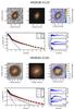 |
Fig. 15 Same as Fig. 2 for the remaining galaxies. |
| In the text | |
|
Fig. 15 continued. |
| In the text | |
|
Fig. 15 continued. |
| In the text | |
|
Fig. 15 continued. |
| In the text | |
|
Fig. 15 continued. |
| In the text | |
|
Fig. 15 continued. |
| In the text | |
|
Fig. 15 continued. |
| In the text | |
|
Fig. 15 continued. |
| In the text | |
|
Fig. 15 continued. |
| In the text | |
|
Fig. 15 continued. |
| In the text | |
Current usage metrics show cumulative count of Article Views (full-text article views including HTML views, PDF and ePub downloads, according to the available data) and Abstracts Views on Vision4Press platform.
Data correspond to usage on the plateform after 2015. The current usage metrics is available 48-96 hours after online publication and is updated daily on week days.
Initial download of the metrics may take a while.