| Issue |
A&A
Volume 561, January 2014
|
|
|---|---|---|
| Article Number | A48 | |
| Number of page(s) | 20 | |
| Section | Planets and planetary systems | |
| DOI | https://doi.org/10.1051/0004-6361/201322453 | |
| Published online | 23 December 2013 | |
Pulsation analysis and its impact on primary transit modeling in WASP-33⋆,⋆⋆
1
Hamburger Sternwarte, University of Hamburg,
Gojenbergsweg 112,
21029
Hamburg,
Germany
e-mail:
This email address is being protected from spambots. You need JavaScript enabled to view it.
2
Department of Astronomy, University of Texas,
Austin, TX
78712,
USA
3
Institut de Ciències de l’Espai (CSIC-IEEC), Campus UAB, Facultat
de Ciències, Torre C5 parell, 2a
pl, 08193
Bellaterra,
Spain
4
Leibniz-Institut für Astrophysik Potsdam,
An der Sternwarte
16, 14482
Potsdam,
Germany
5
Dept. d’Astronomia i Meteorologia, Institut de Ciències del Cosmos
(ICC), Universitat de Barcelona (IEEC-UB), Martí Franquès 1, 08028
Barcelona,
Spain
6
Institut für Astrophysik der Universität Wien,
Türkenschanzstr. 17,
1180, Wien,
Austria
Received:
6
August
2013
Accepted:
19
October
2013
Abstract
Aims. To date, WASP-33 is the only δ Scuti star known to be orbited by a hot Jupiter. The pronounced stellar pulsations, showing periods comparable to the primary transit duration, interfere with the transit modeling. Therefore our main goal is to study the pulsation spectrum of the host star to redetermine the orbital parameters of the system by means of pulsation-cleaned primary transit light curves.
Methods. Between August 2010 and October 2012 we obtained 457 h of photometry of WASP-33 using small and middle-class telescopes located mostly in Spain and in Germany. Our observations comprise the wavelength range between the blue and the red, and provide full phase coverage of the planetary orbit. After a careful detrend, we focus our pulsation studies in the high frequency regime, where the pulsations that mostly deform the primary transit exist.
Results. The data allow us to identify, for the first time in the system, eight significant pulsation frequencies. The pulsations are likely associated with low-order p-modes. Furthermore, we find that pulsation phases evolve in time. We use our knowledge of the pulsations to clean the primary transit light curves and carry out an improved transit modeling. Surprisingly, taking into account the pulsations in the modeling has little influence on the derived orbital parameters. However, the uncertainties in the best-fit parameters decrease. Additionally, we find indications for a possible dependence between wavelength and transit depth, but only with marginal significance. A clear pulsation solution, in combination with an accurate orbital period, allows us to extend our studies and search for star-planet interactions (SPI). Although we find no conclusive evidence of SPI, we believe that the pulsation nature of the host star and the proximity between members make WASP-33 a promising system for further SPI studies.
Key words: asteroseismology / instrumentation: photometers / planet-star interactions / methods: observational / techniques: photometric / stars: variables:δScuti
Tables 1 and 10 and Fig. 8 are available in electronic form at http://www.aanda.org
Photometry is only available at the CDS via anonymous ftp to cdsarc.u-strasbg.fr (130.79.128.5) or via http://cdsarc.u-strasbg.fr/viz-bin/qcat?J/A+A/561/A48
© ESO, 2013
1. Introduction
The first mention of δ Scuti variability was made more than one hundred years ago (Campbell & Wright 1900). Fifty years later, Eggen (1956) pointed out the need to place these variable stars under an independent stellar classification. The δ Scutis have been among us for a long time. Nevertheless, because of the intrinsically small variability near the limit of detectability major studies of them did not begin until the 1970s (Baglin et al. 1973; Breger 1979; Breger & Stockenhuber 1983). Nowadays, the Kepler telescope alone provides precise light curves of several hundred δ Scuti stars (e.g., Uytterhoeven et al. 2011).
In the Hertzsprung-Russell diagram, the δ Scuti stars are located in an instability strip covering spectral types between A and F (Baglin et al. 1973; Breger & Stockenhuber 1983). Most δ Scuti stars belong to Population I (Breger 1979), with typical masses of 2 M⊙ (Milligan & Carson 1992). Due to both radial and nonradial pulsations, δ Scuti stars show brightness variations from milli-magnitudes up to almost one magnitude in blue bands. In δ Scuti stars, pulsations are driven by opacity variations. There are two distinct types of pulsation modes that might occur (e.g., Breger et al. 2012): short-period p-modes (pressure modes, for which pressure serves as the restoring force) and long-period g-modes (gravity modes, with buoyancy as the restoring force). A typical δ Scuti pulsation spectrum shows dozens of periods (Breger et al. 1999a,b), with cycle durations ranging from a couple of hours to the minute regime.
WASP-33 (HD 15082) is a bright (V ~ 8.3), rapidly rotating (vsin(i) ~ 90 km s-1)1δ Scuti star; in fact, it is both the hottest and only δ Scuti star known to date to host a hot Jupiter (Christian et al. 2006). The planet, WASP-33b, was detected through its transits in the frame of the WASP campaign (Pollacco et al. 2006). It circles its host star every 1.22 d in a retrograde orbit. With a brightness temperature of 3620 K, WASP-33b is the hottest exoplanet known to date (Smith et al. 2011). Showing an unusually large radius, WASP-33b belongs to the class of anomalously inflated exoplanets (Collier Cameron et al. 2010). For its mass and hence density, only an upper limit of Msin(i) < 4.59 MJ2 has been determined.
The host star, WASP-33A, shows pronounced pulsations with periods on the order of one hour. Collier Cameron et al. (2010) note that the presence of these pulsations offers “the intriguing possibility that tides raised by the close-in planet may excite or amplify the pulsations in such stars”. The discovery of WASP-33’s pulsations within photometric data were first reported by Herrero et al. (2011), who suggest a possible commensurability between a pulsation period and the planetary orbital period with a factor of 26, indicative of SPI.
We study the pulsations and primary transits using a total of 56 light curves of WASP-33, observed during two years and providing complete orbital phase coverage.
2. Observations and data reduction
Between Aug. 2010 and Oct. 2012, we obtained 457 h of photometry of WASP-33 distributed across 56 nights using six telescopes: one in Germany and five in Spain. Figure 1 shows the temporal coverage provided by the individual telescopes; the details of the observations are given in Tables 1 and 2 and the technical characteristics of the telescopes are summarized in Table 3.
Throughout the analysis, the barycentric dynamical time system is used (BJDTDB). Conversions between different time reference systems have been carried out using the web-tool made available by Eastman et al. (2010)3.
WASP-33 is located in a sparse stellar field. Therefore the defocusing technique did not produce any undesired effect, such as overlapping of the stellar point spread functions. However, after either defocusing or considering the natural seeing of the sites, the optical companion identified by Moya et al. (2011) is contained, in most of the cases, inside the selected aperture radius. A discussion on third-light contribution is addressed in Sect. 4.
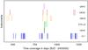 |
Fig. 1 Sampling of our observations. |
Overview of observation nights for CAHA, OADM, OMNP, and OMCB.
Technical telescope data: primary mirror diameter, field of view (FOV), plate scale, and observatory location.
2.1. Hamburger Sternwarte
The Oscar Lühning Telescope4 (OLT) is located at the Hamburger Sternwarte, Germany. It is equipped with an Apogee Alta U9000 charge-coupled device (CCD) camera with guiding system.
Between Nov. 2010 and Oct. 2012, we observed WASP-33 for 29 nights using the Johnson-Cousins B and R filters (see Table 1 for details). The exposure time was between 10 and 40 s, mainly depending on the night quality. The airmass ranged from principally 1 to 3 only when photometric nights allowed such observations. The typical seeing at the Hamburger Sternwarte is 2.5−3 arcsec. Therefore saturation was not an issue. During a total time of ~150 h, we obtained 18 090 photometric data points providing both in- and out-of-transit coverage. Additionally, calibration frames were obtained for each individual night.
For bias subtraction and flat fielding, we used the ccdproc package in IRAF; aperture photometry was carried out using IRAF’s apphot. To obtain differential photometry, we measured unweighted fluxes in WASP-33 and two reference stars using various aperture radii. The final light curve was produced using the aperture that minimizes the scatter of the differential light curve. It is based on the brighter of the two reference stars, BD+36 488, which is, however, still one magnitude fainter than WASP-33. The remaining reference star was used to obtain control light curves to ensure that the photometry is based on a proper reference.
2.1.1. Calar Alto observatory
The German-Spanish Astronomical Center at Calar Alto (CAHA) is located close to Almería, Spain. It is a collaboration between the Max-Planck-Institut für Astronomie (MPIA) in Heidelberg, Germany, and the Instituto de Astrofísica de Andalucía (CSIC) in Granada, Spain.
We used the Bonn University Simultaneous CAmera (BUSCA)5 instrument, which is mounted at the 2.2 m telescope. The instrument allows simultaneous measurements in four different spectral bands. To reduce read-out time, we exposed only the half-central part of the CCD. We observed WASP-33 using the Strömgren v, b, and y filters, along with a filter labeled d, which is centered at 753 nm with a FWHM of 30 nm. As BUSCA requires simultaneous read-out of all CCDs, we used an exposure time of 4 s, which provides adequate signal-to-noise ratios in the Strömgren bands and avoids saturation of the source. The photometry obtained by means of the d filter was discarded due to low signal-to-noise. During our observations, the seeing ranged between 1 and 1.5 arcsec. In the visible, the extinction was between 0.15 and 0.2 mag/airmass. Observing for ~23 h, we obtained 927 photometric data points per filter. The data reduction was carried out as described in Sect. 2.1.
2.2. Observatorio del Teide
STELLar Activity (STELLA)6 consists of two fully robotic 1.2 m telescopes, one dedicated to photometry and the other to spectroscopy (Strassmeier et al. 2010). The photometer is a wide-field imager called WiFSIP. It is equipped with a 40922 15-μm pixel back-illuminated CCD.
We observed WASP-33 using STELLA for one month starting at the end of Oct. 2011. STELLA’s optical setup offers a field of view of 22′ × 22′. However, for the purposes of these observations and with the main goal of reducing readout times, we used only a 15′ × 15′ subframe. To obtain quasi-simultaneous multiband photometry, we alternated between the Strömgren v and b filters. In this way, we obtained 2483 photometric measurements with the v filter and 2234 with the b filter, which equates to ~75 h per spectral range. Accounting for read-out time, the typical temporal cadence was of ~90 s. The optics had to be defocused to avoid saturation of the target.
We carried out the data reduction using ESO-MIDAS. Bias frames were obtained every night, evening, and morning and combined into a master bias on a daily basis. Twilight flat-field frames for both the Strömgren b and v filters were obtained approximately every 10 d. Bias subtraction and flat-fielding were performed as usual. We carried out aperture photometry using SExtractor’s MAG AUTO option. Here, SExtractor computes an elliptical aperture for every detected object in the field, following its light distribution in x and y, and scales the aperture width with the SExtractor parameter k, which we set to 2.6. As a flux calibrator, we used the summed, unweighted flux of three reference stars, viz., BD+36 493, BD+36 487, and BD+36 488. The background, estimated locally for each object, was generally low.
2.3. Primary transit observations
To increase our sample of primary transit light curves, we used three telescopes with apertures between 0.3 and 0.8 m. To carry out the observations we defocused the telescopes. In the particular case of bright sources such as WASP-33, long exposures after defocusing can reduce scintillation noise and flat-fielding errors (e.g., Southworth et al. 2009; Gillon et al. 2009). In this way, we reached milli-magnitude precision in all of the primary transit light curves obtained using small-aperture telescopes.
The Telescopi Joan Oró is a fully robotic telescope located at the Observatori Astronòmic del Montsec7 (OADM). It is equipped with an FLI Proline 4240 CCD and standard Johnson-Cousins filters. Observing for five nights distributed over two years, we collected 19.4 h of data at a temporal cadence of ~45 s.
The Observatori Montcabrer8 (OMCB) is located in Cabrils, Spain. We used its remotely operated 0.3 m telescope, which is equipped with an SBIG ST-8 CCD and standard Johnson-Cousins filters for seven nights distributed over 1.5 yr. In total, we collected ~40 h of data with typical exposure times of ~120 s. Although the observatory is located in a light-polluted area, a photometric precision of about 1 mmag could be reached.
The Observatori Món Natura Pirineus9 (OMNP) contributed a 0.4 m telescope equipped with an SBIG STL-1001E CCD. With this telescope we observed one primary transit using the Johnson-Cousins V filter.
The data of all the telescopes were corrected for bias and dark current and were flat-fielded using MaximDL and new calibration images for every night. The light curves were produced using Fotodif10. In all cases, the aperture radius was selected such that the scatter in the out-of-transit sections of each light curve is minimized.
3. WASP-33 as a δ Scuti star
The primary transit light curves of WASP-33 are deformed by the host star’s pulsations. This interferes with transit modeling and therefore with the determination of the orbital and physical parameters of the system. As the removal of an inappropriate primary transit model could introduce a spurious signal in the pulsation spectrum of the star, associated with the planetary orbital period rather than intrinsic stellar variability, we use only off-transit data points to determine WASP-33A’s pulsation spectrum.
The pulsation frequency analysis is performed using PERIOD04, a package intended for the statistical analysis of large astronomical data sets containing gaps, with single-frequency and multiple-frequency techniques (Lenz & Breger 2005). The package utilizes both Fourier and multiple-least-squares algorithms, which do not rely on sequential prewhitening or assumptions of white noise.
3.1. Light curve normalization
To avoid variations apart from the periodicity that we want to characterize, the light curves need to be first detrended. Thus, to study the pulsation spectrum in the high-frequency regime, we normalize each individual light curve. In this way, we eliminate the low-frequency signals that might be associated with systematic effects, such as residual fluctuations due to atmospheric extinction, that are unrelated to intrinsic stellar variability.
Our procedure is the following: first, we bin the light curves using time-bins with a duration of ~1.3 h to “hide” the high-frequency pulsations inside them. Second, we calculate the mean value of time and flux in the bins and fit a low-order polynomial to the binned light curves. The degree of the polynomial depends on the number of available data points and therefore on the duration of the observing night. Finally, we subtract the fitted polynomial from the unbinned light curve and convert magnitudes into flux. To ensure a proper normalization, we visually inspected the results of our procedure. Figure 2 shows a representative example.
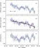 |
Fig. 2 Our normalization procedure: a) Differential light curve in magnitudes, obtained using the STELLA telescope and the Strömgren v filter. The length of the arrow indicates the width of the time-bins. b) Thick red points: the binned time, flux, and photometric error. Continuous black line: third-degree polynomial fitted to the binned data points. c) Normalized light curve in flux units. |
3.2. Light curve normalization and its relevance for periodogram analysis
To study the impact of the normalization on the high-frequency domain, we applied an alternative normalization and subtracted only the mean value of the light curves. We then compared the periodograms obtained for each data set based on the two normalizations. Figure 3 shows the resulting power spectra for our STELLA data obtained with the Strömgren b filter as an example. The vertical dashed line in the figure indicates the frequency corresponding to the average length of our observing nights. The difference between the periodograms shows how the normalization process affects the power spectrum. The discrepancy is strongest for frequencies corresponding to periods longer than the average night length. Beyond that limit, the effect of the normalization becomes weak. Figure 3 shows close-ups of the periodograms around ν ~ 20 c/d and ν ~ 10 c/d. While the amplitudes of individual peaks change, the structure of the periodogram and the position of the peaks remain stable.
To verify the stability of the peak positions, we searched both periodograms for strong peaks and compared their frequency. To determine the peak positions, we used a Gaussian fit. Based on 66 peak pairs in the >10 c/d regime, we derive a shift of −0.003 ± 0.0025 c/d. At lower frequencies the uncertainty becomes larger, which is in agreement with the behavior observed in Fig. 3. Thus, we conclude that the normalization does not seriously impede the analysis in the high-frequency regime.
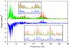 |
Fig. 3 Periodogram for STELLA b data for the polynomial normalization in red, the alternative normalization with a constant in green, and their difference in blue (arbitrarily shifted). The vertical dashed line indicates the mean duration of the observing nights. |
3.3. Determination of WASP-33’s frequency spectrum
Our frequency analysis is based on the STELLA, CAHA, and OLT data. The latter provide a total temporal coverage of approximately two years, essentially concentrated, however, in three observing seasons. Each OLT season was considered separately in our frequency search. We were left with five data sets obtained in four different spectral filters. Although the photometric amplitudes of δ Scuti stars depend on wavelength, it is possible to combine multifilter data to determine the frequencies via Fourier methods. Consequently, we combine the data obtained with the v, B, and b filters, for which we found the difference in amplitude values to be statistically insignificant.
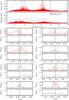 |
Fig. 4 Top panels: periodogram of the combined data set and the final residuals in part per thousand (ppt). The solid line indicates the significance curve. Bottom panels: a closer look at the periodogram around the detected frequencies and the spectral window (SW). Dashed vertical lines around the peaks indicate our error estimates as listed in Table 4. |
We identified the frequencies of the dominating pulsations by analyzing the combined data set, which provides the cleanest spectral window and the highest precision in the determined frequencies.
To estimate the signal-to-noise level of a given pulsation with amplitude Ao, we computed the average amplitude, σres, over a frequency interval with a width of 2 c/d from a periodogram obtained from the final residuals (see Fig. 4) and estimated the amplitude signal-to-noise ratio (ASNR) of each pulsation as Ao/σres. Following Breger et al. (1993), we consider a pulsation to be significant when the estimated ASNR of the periodogram peak is larger than four.
The residual power spectrum indicates strong departures from white noise arising from a potentially highly complex pulsation spectrum and/or aliasing problems. Nonetheless, all remaining peaks remain below our significance curve.
Because we have made annual solutions, the phase and amplitude shifts from year to year have been taken care of. However, if small and systematic changes occur from year to year, there will exist smaller changes within each observing season. Such changes are not taken care of by PERIOD04 and will lead to close side lobes in the periodogram. However, since the solution presented in this work does not contain very close frequencies, these side lobes will not affect it.
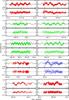 |
Fig. 5 Exemplary off-transit light curves color-coded in red for OLT, green for STELLA, and blue for CAHA, overplotted with the pulsation model in black continuous line. Top panels: normalized flux. Bottom panels: residuals after the pulsation model has been subtracted. |
Strong aliasing represents an unavoidable difficulty, leading to 1 c/d ambiguities and a large number of strong peaks at the 30% level (relative to the main peak). This aliasing, combined with a large number of frequencies, sets the limits of our multifrequency analysis. To minimize the effect of aliasing and the window function on our frequency selection, we checked that the significant peaks are present in all subsamples, where we, however, tolerated lower ASNR levels. As the subsamples comprise only a fraction of the data, the frequencies cannot be determined with the same accuracy as in the combined sample. We obtained estimates of the frequency and the uncertainty (see Sect. 3.4) from the subsamples and verified that the results are consistent with the values obtained using the combined data set. Only if this was the case did we accept a frequency. One frequency near 7.3 c/d, detected in the combined data set, could not be found in all individual data sets and is consequently not included in our analysis.
Altogether, eight frequencies were extracted from the data. Table 4 shows the frequencies, amplitudes, phases, and associated ASNRs. Additionally, we provide the mean frequency and error obtained from the subsamples. Figure 5 shows our pulsation model, plotted over some of the available off-transit light curves. The displayed pulsation model is obtained after fitting the phases to each individual night only. The reasons for this procedure will be given in Sect. 3.5.
3.3.1. Analysis of fit quality
To quantify the improvement in the description provided by our pulsation model, we
calculate the resulting χ2 values for the pulsation model
and a constant,  and
and
 and carry out an
F-test. In particular, we calculate the F-statistics using
and carry out an
F-test. In particular, we calculate the F-statistics using
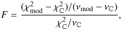 (1)where
ν corresponds to the degrees of freedom,
νmod = 14 701, and
νC = 14 725. Formally, we obtain a
p-value of 1 × 10-16, indicating that the pulsation model
accounts for a substantial fraction of the light curve variations.
(1)where
ν corresponds to the degrees of freedom,
νmod = 14 701, and
νC = 14 725. Formally, we obtain a
p-value of 1 × 10-16, indicating that the pulsation model
accounts for a substantial fraction of the light curve variations.
Although our model reproduces the overall stellar pulsation pattern, the bottom panels of Fig. 5 show flux residuals that do not behave as random, uncorrelated noise. Such residuals may be produced by nonsinusoidal pulsations, low-amplitude pulsations not accounted for in the model or by local changes in the atmospheric conditions not entirely removed by the differential photometry. At any rate, the remaining scatter in the data defines the limiting accuracy achievable in cleaning the primary transits.
3.4. Error treatment
Preliminary error estimates for the frequencies listed in the second column of Table 4 were obtained in two ways. First, we followed the analytical expressions of Breger et al. (1999a). Second, we fitted a Gaussian function to the peaks and used the standard deviation as our error estimate. To be conservative, we used the larger of these as frequency-error estimate. As the residuals show correlated noise, the true uncertainties in our frequencies could be considerably larger. A deeper discussion of errors is given below.
3.4.1. Correlated noise and unevenly spaced data for periodogram analysis
Montgomery & O’Donoghue (1999) present
analytical results of the effect that random, uncorrelated noise has on a least-squares
fit of a sinusoidal, evenly sampled signal. They provide the following expressions for
the uncertainties: 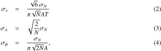 where
σν,
σA, and
σφ are the standard deviations for a
sinusoidal signal with frequency ν, amplitude A, and
phase φ. The remaining parameters are N for the total
number of data points, T for the total duration of the observing
campaign, and σN for the average
measurement error of the data points. If the time series are unevenly sampled and show
correlated noise (e.g., due to atmospheric extinction), Montgomery & O’Donoghue (1999) suggest to estimate errors according to
where
σν,
σA, and
σφ are the standard deviations for a
sinusoidal signal with frequency ν, amplitude A, and
phase φ. The remaining parameters are N for the total
number of data points, T for the total duration of the observing
campaign, and σN for the average
measurement error of the data points. If the time series are unevenly sampled and show
correlated noise (e.g., due to atmospheric extinction), Montgomery & O’Donoghue (1999) suggest to estimate errors according to
 where
where
 is the
variance of the parameter for uncorrelated data sets, given by Eqs. (2)−(4). Further, Δt is the mean exposure time of the data set,
D is an estimate of the number of consecutive correlated data points,
and ω = 2πν is the angular frequency of the pulsation.
is the
variance of the parameter for uncorrelated data sets, given by Eqs. (2)−(4). Further, Δt is the mean exposure time of the data set,
D is an estimate of the number of consecutive correlated data points,
and ω = 2πν is the angular frequency of the pulsation.
An upper limit for the error can be obtained by maximizing Eq. (6). This occurs when the correlation time is on the order of the signal period. In this case, we obtain A = Amax ~ 0.24P/Δt. Table 5 shows the upper-limit uncertainty estimates for our pulsation model parameters, obtained by means of Eq. (5). Here, we used the last column of Table 4 as an estimate for the “uncorrelated” errors. The estimated upper error limits remain satisfactory to characterize the pulsations photometrically.
3.4.2. Photometric errors
The photometric reduction tasks used in this work neglect systematic effects and provide statistical measurement errors, which are rather lower limits to the true uncertainties. We study the impact of the measurement errors on our frequencies analysis, based on the OLT, STELLA, and CAHA data (Johnson-Cousins B filter for OLT and Strömgren v for STELLA and CAHA).
In particular, we randomly increase the photometric errors by a factor of up to two and recalculate the position of the leading peaks and their respective ASNR. After repeating this procedure 104 times, we analyzed the resulting statistics of peak positions and ASNR. We find that the observed change in frequency is contained within the previously derived error. The ASNR decreases but remains higher than ~4 in all cases. Therefore we conclude that our frequency analysis is robust against a moderate increase of up to 100% in the photometric error.
Upper limits for the errors of the pulsation-associated parameters.
3.5. Phase-shift analysis
Photometry provided by the Kepler satellite has widely been used to study the pulsation spectrum and its evolution in δ Scuti stars (e.g., Balona et al. 2012b,a; Southworth et al. 2011; Murphy et al. 2012). Most of the analyzed δ Scuti stars pulsate in several modes. For example, Breger et al. (2012) identify 349 frequencies in the rapidly rotating Sct/Dor star KIC 8054146, for which the authors even find variations in amplitude and phase.
Following the method of Breger (2005) to identify amplitude variations and phase shifts, we divided our off-transit data sets into four subsets: from BJD ~ 2 455 596 to BJD ~ 2 455 641 (~1.5 months), from BJD ~ 2 455 805 to BJD ~ 2 455 837 (~1 month), from BJD ~ 2 455 858 to BJD ~ 2 455 896 (~1 month), and from BJD ~ 2 456 162 to BJD ~ 2 456 217 (~2 months). This particular choice avoids including data gaps due to seasonal effects in the subsamples and therefore limits the impact of aliasing. As the amplitude of WASP-33’s pulsations is too low to identify amplitude variations by means of our photometric data, we focus on phase shifts. In particular, we fit the phases in each subsample, fixing the amplitudes and frequencies to the values listed in Table 4. Figure 6 shows our results. Error bars are on the order of ~0.005 and therefore rather negligible in the plot.
For all eight detected pulsations, we find a change in phase. There are striking similarities between the O−C diagrams of ν2, ν3, ν5, ν7, and ν8, as well as between ν4 and ν6. The largest observed gradient is about 2 × 10⁻³ d-1, assuming a linear evolution. Clearly, such shifts must be taken into account in the construction of a pulsation model to clean the transits.
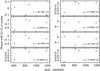 |
Fig. 6 Temporal phase evolution of the pulsation frequencies. |
3.6. Mode identification
A particularly interesting question related to the observed frequencies is their
association with specific pulsation modes, i.e., the radial order, n,
degree, ℓ, and azimuthal number, m, of the underlying
spherical harmonic,  . While the
most reliable method for pulsation mode identification is to analyze the line-profile
variation using high-resolution spectroscopy (Mathias et
al. 1997), our analysis remains limited to photometric data. Nonetheless, we
apply three methods of mode identification based on photometry.
. While the
most reliable method for pulsation mode identification is to analyze the line-profile
variation using high-resolution spectroscopy (Mathias et
al. 1997), our analysis remains limited to photometric data. Nonetheless, we
apply three methods of mode identification based on photometry.
3.6.1. Mode identification based on the pulsation constant Q
The pulsation constant, Q, takes the unique value for any given
pulsation frequency and can be used for mode identification (Breger & Bregman 1975). It is defined by
 ,
with P being the pulsation period and
,
with P being the pulsation period and
 and
and  the mean densities of the star and the Sun. Two important Q-values are
0.033 d and 0.026 d; they correspond to the fundamental and first radial overtone
expected in δ Scuti stars. Expressing the densities as a function of
the radius and eliminating the radius via the luminosity, the expression for
Q can be recast (Breger 1990):
the mean densities of the star and the Sun. Two important Q-values are
0.033 d and 0.026 d; they correspond to the fundamental and first radial overtone
expected in δ Scuti stars. Expressing the densities as a function of
the radius and eliminating the radius via the luminosity, the expression for
Q can be recast (Breger 1990):
 (7)Taking
into account the uncertainties in the stellar parameters, Breger (1990) estimate the uncertainty in the Q-value to be
18%. For WASP-33A, we adopted log (g) = 4.3 ± 0.2,
d = 116 ± 16 pc, and Teff = 7430 ± 100 K
(Collier Cameron et al. 2010). We derived the
absolute bolometric brightness Mbol = 2.85 ± 0.07 using the
expression
Mbol = 42.36−5log (R/R⊙) − 10log (Teff)
(Allen 1973). For the eight pulsation
frequencies in our pulsation model, we derive the Q-values listed in
Table 6; errors have been estimated by error
propagation.
(7)Taking
into account the uncertainties in the stellar parameters, Breger (1990) estimate the uncertainty in the Q-value to be
18%. For WASP-33A, we adopted log (g) = 4.3 ± 0.2,
d = 116 ± 16 pc, and Teff = 7430 ± 100 K
(Collier Cameron et al. 2010). We derived the
absolute bolometric brightness Mbol = 2.85 ± 0.07 using the
expression
Mbol = 42.36−5log (R/R⊙) − 10log (Teff)
(Allen 1973). For the eight pulsation
frequencies in our pulsation model, we derive the Q-values listed in
Table 6; errors have been estimated by error
propagation.
Q values and errors for the eight frequencies found in our data.
Comparing the Q-values to the ones expected in δ Scuti stars (Breger 1998, and references therein), we find that ν1, ν2, ν4, ν5, and ν6 are within the range of radial oscillations. Any further mode identification is not possible via Q-values.
To illustrate the difficulty of assigning modes accurately only by means of the pulsation constant, Q, we compare our most accurate Q6-value with the ones theoretically predicted by Fitch (1981). The model that best matches the WASP-33A parameters is labeled “1.5M21”. Within errors, the following modes correspond to Q6: first, second, and third harmonic (Table 2A, radial modes); p2 and p3 (Table 2B, ℓ = 1 modes); p1, p2, and p3 (Table 2C, ℓ = 2 modes); and p1, p2, and p3 (Table 2D, ℓ = 3 modes). Therefore the only conclusive result is that Q6 corresponds to a p-mode, which is expected for a high-frequency pulsation.
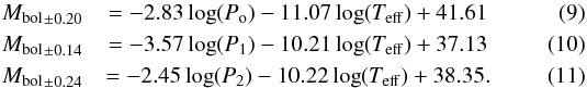
3.6.2. The empirical period-luminosity-color relation
Empirical period-luminosity-color (P-L-C) relations have been studied, e.g., by Petersen & Hog (1998), López de Coca et al. (1990), and King (1991), among many others.
Stellingwerf (1979) derive a theoretical P-L-C
relation  (8)where
P is the period in days and C is a constant equal to 11.96, 11.85,
and 11.76 for the fundamental and first and second harmonics. Substituting our values
for Mbol and Teff, yields
ν0,S = 23.43 c/d,
ν1,S = 30.18 c/d, and
ν2,S = 37.13 c/d, i.e., periods that have
not been identified within our data.
(8)where
P is the period in days and C is a constant equal to 11.96, 11.85,
and 11.76 for the fundamental and first and second harmonics. Substituting our values
for Mbol and Teff, yields
ν0,S = 23.43 c/d,
ν1,S = 30.18 c/d, and
ν2,S = 37.13 c/d, i.e., periods that have
not been identified within our data.
In an observational study, Gupta (1978) finds
that a separate P-L-C relation for each pulsation mode provides a better agreement with
the observations than a general one. The author derived the following empirical P-L-C
relations for the fundamental mode, F (Eq. (9)), and the first, H1 (Eq.
(10)), and second harmonic,
H2 (Eq. (11)):
 These
relations predicts ν0,G = 27.91 c/d,
ν1,G = 29.41 c/d, and
ν2,G = 45.47 c/d, again not observed
within our data. At least for WASP-33A’s stellar parameters, the theoretical and
observational relation seem to be mutually inconsistent.
These
relations predicts ν0,G = 27.91 c/d,
ν1,G = 29.41 c/d, and
ν2,G = 45.47 c/d, again not observed
within our data. At least for WASP-33A’s stellar parameters, the theoretical and
observational relation seem to be mutually inconsistent.
3.6.3. Multicolor photometry
In δ Scuti stars, the photometric amplitude and phase of pulsations depend on the spectral band. The amplitude and phase of a given pulsation are determined by the local effective temperature and cross-section changes, which are defined by the pulsation mode. Therefore different modes lead to distinguishable modulations in flux. This allows mode identification to be carried out by means of multicolor photometry (Balona & Evers 1999; Daszyńska-Daszkiewicz et al. 2003; Dupret et al. 2003).
Frequency Analysis and Mode Identification for Astero Seismology (FAMIAS) is a collection of software tools for the analysis of photometric and spectroscopic time series data (Zima 2008). The photometry module uses the method of amplitude ratios and phase differences in different photometric passbands to identify the modes (Balona & Stobie 1979; Watson 1988). The determination of the ℓ-degrees is based on static plane-parallel models of stellar atmospheres and on linear non-adiabatic computations of stellar pulsations. To compute the theoretical photometric amplitudes and phases, FAMIAS applies the approach proposed by Daszyńska-Daszkiewicz et al. (2002).
FAMIAS requires the stellar parameters’ effective temperature, Teff, surface gravity, log g, and metallicity, [Fe/H], which we obtained from Collier Cameron et al. (2010). As additional input to FAMIAS, we obtained the pulsation frequency, the amplitude, and the phase for the Strömgren v and b bands using our STELLA and CAHA data; amplitude ratios and phase differences were obtained using PERIOD04. Figure 7 shows our results for the case of ν2, ν4, and ν5. The pulsations seem to correspond to lower-order modes: ℓ = 0, 1 for ν5 and ν4, and ℓ = 2, 3 for ν2. A more detailed characterization of these modes results impossible in our analysis. For the remaining five frequencies in our model, no reliable information on the associated modes could be derived.
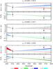 |
Fig. 7 Amplitude ratios and phase differences in degrees relative to the Strömgren v filter for WASP-33, resulting from the three available nights obtained at Calar Alto. The filled curves indicate the uncertainty of the theoretical prediction due to observational errors in Teff and log g. |
3.6.4. The effect of rotation
Any asteroseismological study of main-sequence δ Scuti stars is not completely fulfilled until stellar rotation is considered (Goupil et al. 2000, and references therein). The effects of rotation over the pulsation spectrum has been theoretically studied (e.g., Deupree 2011; Deupree et al. 2012), as well as observed (e.g., Breger et al. 1999b, 2005, 2012). The main effect of rotation is the splitting of the nonradial mode frequencies. If such splitting is observed, then the rotation rate of a star can be determined (Christensen-Dalsgaard & Berthomieu 1991).
From a purely geometrical argument, stellar rotation affects the observed frequencies.
In an inertial frame, an observer finds that a frequency is split uniformly according to
the azimuthal order m:
 (12)where Ω is the
angular velocity of the star, νo is the frequency of the
pulsation in the frame rotating with the star, and m the azimuthal
mode. Using this simplified version of mode splitting (see, e.g., Cowling & Newing 1949, for the contribution of Coriolis
forces to the frequency splitting), we produced the following analysis: from the eight
frequencies that conform to our pulsation model, we assume that one of them,
νj,m, is the product of mode splitting.
Therefore knowing that the azimuthal order m is associated with
νj,m and the rotational period of the
star, we can determine νo. With
νo, we can further calculate the values of the remaining
νj,ms for a given ℓ
degree (| m| < ℓ), and
compare them with our remaining model frequencies.
(12)where Ω is the
angular velocity of the star, νo is the frequency of the
pulsation in the frame rotating with the star, and m the azimuthal
mode. Using this simplified version of mode splitting (see, e.g., Cowling & Newing 1949, for the contribution of Coriolis
forces to the frequency splitting), we produced the following analysis: from the eight
frequencies that conform to our pulsation model, we assume that one of them,
νj,m, is the product of mode splitting.
Therefore knowing that the azimuthal order m is associated with
νj,m and the rotational period of the
star, we can determine νo. With
νo, we can further calculate the values of the remaining
νj,ms for a given ℓ
degree (| m| < ℓ), and
compare them with our remaining model frequencies.
Although this approach might sound straight forward, there is no knowledge of the rotational period of WASP-33A. We therefore assumed that WASP-33A’s vsin(i) is coincident with the equatorial velocity. Furthermore, our attempt to identify the nature of the observed frequencies did not produce any substantial results. Consequently, for our most accurately identified ν2 frequency (ℓ = 2, 3) we assumed all possible m values and found, through this reasoning, that the remaining observed frequencies were not the product of mode splitting.
Any further study would require, for instance, a complete mode identification and the knowledge of the rotational period of the star. The complexity around mode identification clearly indicates that Q values, P-L-C relations, rough period ratios, and even poor mode identification via multicolor photometry cannot be used for mode identification without further evidence.
Summary of our primary transit observations and modeling parameters.
4. Primary transit analysis
Our data comprise 19 primary transit observations. Table 7 lists, among others, the date and site of observation, the filter, and a code indicating the transit coverage of the observation. To determine the orbital parameters, we focus on the eight primary-transit light curves providing complete temporal coverage (TC = OIBEO in Table 7).
Moya et al. (2011) report on the detection of an optical companion about ~2′′ from WASP-33, which could affect our observations through third-light contamination. Based on the color information (Jc, Hc, Kc, and FII filters), the authors speculate that it might be a physical companion of WASP-33, for which they estimate an effective temperature of Teff = 3050 ± 250 K. As the third-light contribution provided by such an object is ≲4 × 10⁻⁴ in all used filters, it can be neglected in our analysis.
Orbiting a fast rotator in a quasi polar orbit (projected spin-orbit misalignment
λ ~ 255°, Collier Cameron et
al. 2010), the transit’s light curves may be affected by gravity darkening, which
manifests in a latitudinal dependence of the stellar effective temperature (von Zeipel 1924). As the rotational period of WASP-33 is
unknown, we estimate it using vsin(i) ~ 90
km s-1 and the stellar radius
Rs ~ 1.44 R⊙ (Collier Cameron et al. 2010). Close to the system
geometry, we estimate the polar-to-equatorial temperature ratio. Using a gravity-darkening
exponent of β = 0.18 (Claret 1998),
for g the magnitude of the local effective surface gravity, and
β the gravity-darkening exponent, following Maeder (2009):  (13)
(13)
we estimate that the polar temperature of WASP-33 is ≈2.2% higher than the equatorial temperature. This is too small to reproduce the observed transit depth wavelength-dependent variation. Further, using the primary transit code of Barnes (2009), which is adequate for fast rotators, we determine that the differences in the transit shape observed in the blue and red bands caused by gravity darkening are on the order of 0.06% and therefore negligible in our analysis. Therefore the occultquad routine provided by Mandel & Agol (2002) is adequate for our transit modeling.
4.1. Photometric noise
Often, the scatter in the light curve is used as a noise estimate. If, however, correlated noise is present, this method may considerably underestimate the impact of the scatter on the parameter estimates. The effect of correlated noise on transit modeling has been studied by several authors, e.g., Carter & Winn (2009); Pont et al. (2006).
While we have identified the significant pulsations in Sect. 3, our analysis has also shown that there is an unknown number of weak pulsations that we cannot account for in our modeling. The unaccounted pulsations will manifest in time-correlated noise in the transit analysis. Therefore a treatment of time-correlated noise is important in the transit modeling.
To quantify the amplitude of time-correlated noise in our data, we applied the “time-averaging method” proposed by Pont et al. (2006), which is based on the comparison of the variance of binned and unbinned residuals. To obtain the residuals, we normalized the transit light curves by fitting a polynomial to the out-of-transit data and then subtracted a preliminary transit model. We verified that the results only slightly depend on the details of the normalization and transit model.
Subsequently, the residual light curves were divided into M bins of equal duration. Each
bin contains N data points. As our data are not always equally spaced, we applied a mean
value for the number of data points per bin. In the absence of red noise, the expectation
value of the variance of the unbinned residuals, σ1, is
related to the variance of the binned residuals,
σN, according to (cf. Carter & Winn 2009, Eq. (36))
 (14)This may now be compared
with a variance estimate,
(14)This may now be compared
with a variance estimate,  , derived from
the binned residuals
, derived from
the binned residuals  (15)If correlated noise
is present, then will differ
from σN by a factor
βN, which estimates the strength of
correlated noise. A proper estimator, β, may be found by averaging
βN over a range Δn
corresponding to the most relevant timescale. To account for the correlated noise in a
conventional white-noise analysis, the individual photometric errors are enlarged by a
factor of β. If there is no prior information, this leaves the parameter
estimates unaffected and enlarges the errors by a factor β.
(15)If correlated noise
is present, then will differ
from σN by a factor
βN, which estimates the strength of
correlated noise. A proper estimator, β, may be found by averaging
βN over a range Δn
corresponding to the most relevant timescale. To account for the correlated noise in a
conventional white-noise analysis, the individual photometric errors are enlarged by a
factor of β. If there is no prior information, this leaves the parameter
estimates unaffected and enlarges the errors by a factor β.
In the case of our transit analysis, the relevant timescale is the duration of ingress or egress, which is ~16 min for WASP-33. In Table 7 we show the resulting β factors. In a first step, we deliberately ignored our results derived in Sect. 3 and treated the light curves as if we had no knowledge on the pulsations. In the thus derived β1 values, all pulsations show up as correlated noise. In a second step, we subtracted the pulsation model derived in Sect. 3 and determined the β2 values. Taking into account the pulsation model always yields a better, that is, smaller β factor, indicating that the model accounts for a substantial fraction of the time correlation.
4.2. Polynomial order of transit light curve normalization
In transit modeling, normalization of the light curves is crucial. To normalize the transit light curves, we fit polynomials with an order between zero and four to the out-of-transit data and determine the order, k, that minimizes the Bayesian information criterion, BIC = χ2 + klnN.
The order of the resulting optimal polynomial is listed in Table 7. According to our modeling, a constant or linear model is sufficient to normalize the transit in all but two cases, where a quadratic normalization is required. Finally, we visually inspected the resulting light curves to ensure a proper normalization.
4.3. Transit modeling
Collier Cameron et al. (2010) detect the planetary “shadow” of WASP-33b in the line profile of WASP-33A during transit. Their spectroscopic time series analysis reveals that the planet traverses the stellar disk at an inclination angle incompatible with 90°. As the inclination is less affected by parameter correlations in the spectroscopic analysis, we impose a Gaussian prior on the inclination. In particular, we use the value of i = 87.67 ± 1.8 deg obtained by Collier Cameron et al. (2010) in their combined photometric and spectroscopic analysis.
In our analysis, we fixed the linear and quadratic limb-darkening coefficients, u1 and u2, to the values listed in Table 8. We obtained these values, which consider the stellar parameters log (g) = 4.5, Teff = 7500, and [Fe/H] = 0.1, from Claret & Bloemen (2011). Therefore we are left with the following free parameters: the mid-transit time, To, the orbital period, Per, the semimajor axis in stellar radii, a/Rs, the orbital inclination, i, and the planet-to-star radius ratio, p = Rp/Rs. As previously mentioned, we used complete primary transits only to determine the best-fit orbital parameters.
Linear (u1) and quadratic (u2) limb-darkening coefficients.
To obtain the parameter estimates, their errors, and mutual dependence, we sample from the posterior probability distribution using an Markov chain Monte Carlo (MCMC) approach. For the parameters a, p, Per, and To, we defined uniform priors covering a reasonable range. Errors are given as 68.3% highest probability density (HPD) credibility intervals. To carry out MCMC sampling, we used Python routines of PyAstronomy 11, which provide a convenient interface to fit and sample algorithms implemented in the PyMC (Patil et al. 2010) and SciPy (Jones et al. 2001) packages.
In a first attempt to fit the transits, we ignore the pulsations and fit only the transit light curves. In our approach, the complete transit light curves are fitted simultaneously using the model of Mandel & Agol (2002). We note that we also fitted the coefficients of the normalizing polynomial, whose degree remains, however, fixed to that listed in Table 7. Our best-fit solutions, which are obtained after 5 × 10⁵ iterations, are given in Table 9.
In a second attempt, we combine the primary transit model with the pulsation model with frequencies and amplitudes fixed to the values listed in Table 4. In Sect. 3.5, we demonstrate that there is a temporal evolution in the phases. Therefore the phases have been considered free parameters in our modeling. However, we did not allow them to take arbitrary values but restricted the allowed range to the limiting cases derived in Sect. 3.5. For instance, the phase of the first frequency, ν1, could not deviate by more than 0.1 cycle from the mean value (cf. Fig. 6).
The results are presented in the lower part of Table 9; in Fig. 8 we show the 19 primary transit light curves and the best-fit model. Interestingly, the parameters derived using this more elaborate approach are consistent with those obtained ignoring the pulsations. Taking into account the pulsation model does, however, improve the uncertainties in the parameter estimates with respect to the regular primary transit-fitting approach.
The values derived in our analysis are broadly consistent with those derived previously by Collier Cameron et al. (2010) and Kovács et al. (2013). While we find a slightly smaller semimajor axis than Collier Cameron et al. (2010)’s, the planet-to-star radius ratio and the inclination are compatible. Kovács et al. (2013) find an 8−10% larger radius ratio and a slightly lower inclination. A homogeneous study of all the primary transits available in the bibliography escapes the purpose of this work. However, we believe that the small differences in the orbital parameters observed by different authors might be the product of an inadequate normalization of the primary transits or an insufficiently correlated noise treatment.
Orbital parameters of WASP-33.
4.3.1. Impact of the pulsations on the transit fits
To better understand the effect of the pulsations on the transit fits, we fit the 19 primary transits individually and study the behavior of a, i, and p. We carry out the fit one more time first ignoring the pulsations and then taking them into account via our pulsation model. During the fit, the ephemeris were fixed to the corresponding values in Table 9. The outcomes are based on 5 × 10⁵ iterations of the MCMC sampler; they are given in Table 10.
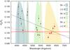 |
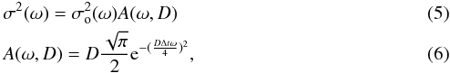
Fig. 9 Planet-to-star ratio |

To study the impact of the pulsation model on the individual parameters, we scrutinized the ratio of the derived values. In particular, we focused on the eight complete transits whose parameters can be determined most reliably. For the ratios of values determined with pulsations considered in the model (wp) and neglected pulsations (pn), we obtained awp/apn = 1.0 ± 0.02, iwp/ipn = 1.000 ± 0.001, and pwp/ppn = 0.99 ± 0.03. These numbers indicate that, on average, the parameter estimates remain unaffected by taking into account the stellar pulsations. Regarding individual fits, the expected deviation amounts to 0.08 Rs in the semimajor axis, 0.1° in the inclination, and 3 × 10⁻³ in p. Clearly, the relative uncertainty is largest in the semimajor axis and the radius ratio, p. Also taking into account the transits with incomplete observational coverage, we obtain numbers that are comparable but with larger uncertainties. It is worth mentioning that the “outlying” orbital parameters, which are presented in Table 10, are the product of incomplete primary transit fitting. Therefore we believe that primary transit normalization might play a fundamental role in the determination of such parameters.
4.4. Wavelength dependence of the planet-to-star radius ratio
Our data comprise transit observations from the blue to the red filter. To check whether
a dependence of the planet-to-star radius ratio on the wavelength can be identified, we
fixed all parameters but the radius ratio to the values listed in Table 9 and fitted only the radius ratio,
 ,
for each individual transit. The resulting
values, which are based on the pulsation-corrected light curves, are listed in the last
column of Table 9. We verified that we obtain
comparable results if the pulsations are not considered.
,
for each individual transit. The resulting
values, which are based on the pulsation-corrected light curves, are listed in the last
column of Table 9. We verified that we obtain
comparable results if the pulsations are not considered.
Figure 9 shows
as a function of wavelength. The red points mark the transits with full observational
coverage, while the black points were derived from transits with incomplete temporal
coverage (see Table 7). In the fit, we used the
central wavelength of the filters, which are indicated by vertical, dashed lines in the
plot. To produce a less crowded figure, the data points are artificially shifted from the
central wavelength.
The values for ,
which are derived from the complete transits, show a wavelength-dependent trend, but only
with marginal significance. These values are also consistent with a constant radius ratio
of
RP/RS = 0.1061 ± 0.0031,
in concordance with the mean value and the standard deviation of the eight data points.
Both the linear and constant models produce comparable
 values of 1.9
and 1.8, respectively. Hence, it is unclear which model best fits the data. If all transit
observations are taken into account, the data indicate a decrease of 0.65%/1000 Å in the
planet-to-star radius ratio with wavelength. Formally, the correlation coefficient between
radius-ratio and wavelengths amounts to r ~ 0.7. We caution, however,
that the observed trend may be feigned by an inappropriate transit normalization because
many transits lack full observational coverage.
values of 1.9
and 1.8, respectively. Hence, it is unclear which model best fits the data. If all transit
observations are taken into account, the data indicate a decrease of 0.65%/1000 Å in the
planet-to-star radius ratio with wavelength. Formally, the correlation coefficient between
radius-ratio and wavelengths amounts to r ~ 0.7. We caution, however,
that the observed trend may be feigned by an inappropriate transit normalization because
many transits lack full observational coverage.
Kovács et al. (2013) also notice a substantial difference in the transit depth derived from an observation in Hα and a simultaneously obtained J-band light curve (their Fig. 9). In particular, the J-band transit is shallower, which would be consistent with the wavelength trend. However, the signature observed through the Hα line may significantly differ from those observed in broadband filters because the Hα line is affected by strong chromospheric contributions.
5. Discussion
5.1. The stellar pulsation spectrum
The pulsation spectrum of WASP-33 has been studied by several authors, who report a wealth of frequencies (see Table 11). All studies find pulsations with amplitudes on the order of 1 mmag, which is compatible with our results.
Deming et al. (2012) observed WASP-33 during two secondary transits in the Ks band using the 2.1 m telescope at Kitt Peak National Observatory and for another two nights using the Spitzer telescope. All observations were performed during secondary transits. Their frequency analysis was carried out for individual nights. Their first three frequencies (21.1, 20.2, and 9.8 c/d) are compatible with our ν1, ν2, and ν3 (see Table 4). Also, de Mooij et al. (2013) observed secondary transits of WASP-33b in the Ks band for two nights, each lasting ~5 h. Although the frequencies they report are within the range of values we find, the values are numerically inconsistent with our results.
Herrero et al. (2011) observed for nine nights mainly during primary transit using Johnson-Cousins R filter. They report pulsation frequencies, which might correspond to our ν1. Smith et al. (2011) carried out observations during one secondary transit using an S[III] narrow-band filter centered at 9077 Å. The observations were performed for almost nine hours during a single night lacking photometric conditions. Among the pulsation frequencies they find, 21.6 ± 0.6 c/d and 34.3 ± 0.4 c/d likely correspond to our ν2 and ν6.
The most extensive pulsation analysis is carried out by Kovács et al. (2013). It is based on four photometric datasets, including that of Herrero et al. (2011). Kovács et al. (2013) report two frequencies that are compatible with our ν1 and ν2. The ~15.2 c/s frequency does not show up in our analysis.
Among the different data sets, pulsations with frequencies around ~21 c/d and ~20 c/d that correspond to our most pronounced frequencies ν1 and ν2 consistently occur. Other pulsation frequencies are only found in some cases. We note, however, that the data were acquired in different spectral bands, mostly in the infrared, where pulsations are expected to be lower in amplitude. The residuals after subtracting our pulsation model clearly indicate the presence of further low-amplitude pulsations, which might correspond to those found in previous studies. Additionally, our phase shift analysis in Sect. 3.5 has shown that the pulsation spectrum might be intrinsically variable. The amplitudes of the pulsations found by the various studies are all on the order of 1 mmag, which is compatible with our results. As the amplitudes are intrinsically small and furthermore wavelength dependent, we refrain from a detailed comparison of the derived numbers.
Evolution of the reported frequencies and amplitudes for WASP-33’s pulsation spectrum (from top to bottom).
In our analysis, we identify eight significant pulsation frequencies. Although the pulsation spectrum is probably much more complex than that, the amplitudes of the pulsations are intrinsically low and more data is required to characterize the components in further detail. We show that the pulsation phases vary in time with a gradient, dp, of up to | dp| ≲ 2 × 10⁻³ d-1, assuming a linear evolution. This suggests that the amplitudes and frequencies also show temporal variability. However, our data do not allow to verify this.
We find that most of the detected frequencies are likely associated with low-order p-modes. We attempt to further identify the modes using Q values, empirical P-L-C relations, and amplitudes and phases of multicolor photometry. However, we find the detected frequencies to be largely incompatible with all these relations. We argue that this is not uncommon (e.g. Breger et al. 2005).
5.2. Transit modeling
In their analysis of photometric follow-up data, Kovács et al. (2013) find a persistent “hump” in the residuals obtained after subtracting the transit model shortly after mid-transit time. While our residuals clearly show unaccounted pulsations, we do not see any such hump recurring at the same phase. Therefore we find no evidence for a persistent structure on the stellar surface like, e.g., a spot belt as suggested by Kovács et al. (2013).
Although our transit modeling is consistent with a constant star-to-planet radius ratio with respect to wavelength, there may be a slight trend indicating a decrease in the radius ratio as the wavelength increases. Although this would be compatible with the results of Kovács et al. (2013), who find that the radius ratio in the J band is smaller than that observed in Hα, we caution that the formation of the Hα line may be different from that observed in broadband filters – a caveat already mentioned by Kovács et al. (2013). Based on the currently available data, we conclude that a constant planet-to-star radius ratio seems most likely.
5.3. Star-planet interaction
Collier Cameron et al. (2010) report on a nonradial pulsation at a frequency of ~4 c/d, which might be tidally induced by the planet. Unfortunately, this frequency lies outside the sensitivity range of our analysis.
In close binary systems, tidal interaction affects stellar oscillations (e.g., Cowling 1941; Savonije & Witte 2002; Willems 2003). In particular, Hambleton et al. (2013) studied a short-period binary system that presents δ Scuti pulsations and tidally excited modes. In addition to the already known commensurability between the pulsation frequencies and the orbital period of the system, the authors found that the spacing between the detected p-modes was an integer multiple of the system’s orbital frequency. Although it is clear that the nature of WASP-33 does not resemble a short-period eccentric binary system, in order to analyze star-planet interaction we search for commensurability of the detected pulsation frequencies with the planetary orbital period and investigated the spacings between them.
As the exact rotation period of the host star WASP-33A remains unknown, it is not entirely clear how exactly the planet affects the stellar surface in the frame of the star; in particular, the period at which the planet affects the same surface element is unknown for the larger fraction of the stellar surface. However, as the planet orbits in a highly tilted, nearly polar orbit, the stellar poles experience a periodic force with a period identical to once and twice the planetary orbital period. When the planet crosses a pole, the effective gravity on both poles is lowered due to the planetary gravity and orbital motion; the effect is, however, not the same on both poles.
Using our best-fit orbital period of 1.2198675 d, we express the pulsation frequencies in terms of the orbital frequency of the planet. The result is presented in the last column of Table 4, where the ratios of the pulsations and the orbit are displayed. We expect the error in the pulsation frequencies to be considerably larger than those in the orbital period. The closest commensurability is found for the 9.8436 c/d, which corresponds to 12.008 times the orbital frequency.
To assess the significance of such a result, we carry out a Monte-Carlo simulation. In
particular, we randomly generate eight frequencies between 8 and 34, i.e., in the
approximate range of our detected pulsations. The frequencies are dropped out from a
uniform distribution. We then calculate the associated ratio based on the orbital
frequency and finally search for the best match. After 50 000 runs, we find that the
cumulative probability distribution for the minimum distance from an integer frequency
ratio is given by 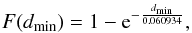 obtained
after fitting our Monte-Carlo results with an exponential decay. Using this relation, we
find that the probability of detecting at least one of the ratios as close or closer than
0.008 c/d to an integer ratio to be 12%. The ratio may indeed be an integer, considering
the error in the frequency determination (see Sect. 3). Nevertheless, we note that our phase-shift analysis also revealed variability
in the frequency spectrum, which we find hard to reconcile with a simple picture of
tidally excited pulsations.
obtained
after fitting our Monte-Carlo results with an exponential decay. Using this relation, we
find that the probability of detecting at least one of the ratios as close or closer than
0.008 c/d to an integer ratio to be 12%. The ratio may indeed be an integer, considering
the error in the frequency determination (see Sect. 3). Nevertheless, we note that our phase-shift analysis also revealed variability
in the frequency spectrum, which we find hard to reconcile with a simple picture of
tidally excited pulsations.
Additionally, we found that the spacing between the frequencies cannot be described by harmonics of the orbital period of the system. In fact, the best case scenario is given by ν5 and ν7. Considering our best-fit orbital period, the departure from an integer number is ten times their estimated error.
Therefore we conclude that there is no evidence for a direct relation between any of our pulsation frequencies and the planetary orbital period.
6. Conclusions
In this work, we obtained and analyzed an extensive set of photometric data of the hottest known star hosting a hot Jupiter, WASP-33. The data cover both in- and out-of-transit phases and are used to study the pulsation spectrum and the primary transits.
In particular, our out-of-transit data provide ~3 times more temporal coverage than the Kovács et al. (2013) data set, which is the most extensive among those listed in Table 11. In addition, our data set is the only one that comprises dedicated out-of-transit photometric coverage to study the stellar pulsations in detail, along with multicolor and simultaneous observations to study the nature of the modes.
A comprehensive study of the pulsation spectrum of WASP-33 reveals, for the first time, eight significant frequencies. Additionally, some of the frequencies found seem to be consistent with previous reports. Along with the associated amplitudes and phases, we construct a pulsation model that we use to correct the primary transit light curves with the main goal of redetermining the orbital parameters by means of pulsation-clean data.
In our transit modeling, we find the system parameters broadly consistent with those reported by Collier Cameron et al. (2010) and Kovács et al. (2013). Interestingly, the derived parameter values are hardly affected by taking into account the pulsations in the modeling although the errors decrease. This statement clearly depends on the total number of observed transits and the stability of the p-modes. Thus further observations of primary transit events of WASP-33 will be required to support or overrule this remark.
One possible explanation of the behavior of the orbital parameters with respect to the pulsations of the host could be that the associated amplitudes, at least in the high-frequency range that our studies focus on, are small in nature. Furthermore, our extensive primary transit observations, which we obtained in different filter bands, allow us to notice a decrease in the planet-to-star radius ratio with wavelength. This decrease has also been observed by other authors. Simultaneous multiband photometry of primary transits of WASP-33 will help to better constrain this dependency.
Considering that our work was produced using fully ground-based observations, we were able to provide an extensive study of the pulsation spectrum of this unique δ Scuti host star. This, in turn, has helped to better comprehend how much pulsations affect the determination of system parameters.
Online material
Overview of observation nights for OLT and STELLA.
Results of individual transit fits.
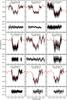 |
Fig. 8 Top panels: the 19 primary transits in black points, along with the photometric error bars accounting for correlated noise, cf. Sect. 4.1. Overplotted in continuous red line is the best-fitted primary transit model modulated by the host star pulsations and the low-order normalization polynomial. Bottom panels: residuals. |
 |
Fig. 8 continued. |
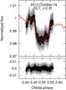 |
Fig. 8 continued. |
i corresponds to the inclination of the stellar rotation axis.
i corresponds to the inclination of the planetary orbit.
Acknowledgments
C. von Essen acknowledges funding by the DFG in the framework of RTG 1351, Dr. Andres Moya and Prof. Rafael Garrido for discussing issues on δ Scuti stars, and the anonymous referee for her/his improvements on the draft. E. H. and I. R. acknowledge financial support from the Spanish Ministry of Economy and Competitiveness (MINECO) and the “Fondo Europeo de Desarrollo Regional” (FEDER) through grant AYA2012-39612-C03-01. The Joan Oró Telescope (TJO) of the Montsec Astronomical Observatory (OAdM) is owned by the Generalitat de Catalunya and operated by the Institute for Space Studies of Catalonia (IEEC). We further thank Ramon Naves for operating the 0.3 m telescope at Observatori Montcabrer, Thomas Granzer for his support on STELLA observations and data reduction, and H. Hagen for his technical support at OLT.
References
- Allen, C. W. 1973, Astrophysical Quantities (London: Athlone Press) [Google Scholar]
- Baglin, A., Breger, M., Chevalier, C., et al. 1973, A&A, 23, 221 [NASA ADS] [Google Scholar]
- Balona, L. A., & Evers, E. A. 1999, Delta Scuti Star Newsletter, 13, 26 [NASA ADS] [Google Scholar]
- Balona, L. A., & Stobie, R. S. 1979, MNRAS, 189, 649 [NASA ADS] [Google Scholar]
- Balona, L. A., Breger, M., Catanzaro, G., et al. 2012a, MNRAS, 424, 1187 [NASA ADS] [CrossRef] [Google Scholar]
- Balona, L. A., Lenz, P., Antoci, V., et al. 2012b, MNRAS, 419, 3028 [NASA ADS] [CrossRef] [Google Scholar]
- Barnes, J. W. 2009, ApJ, 705, 683 [Google Scholar]
- Breger, M. 1979, PASP, 91, 5 [NASA ADS] [CrossRef] [Google Scholar]
- Breger, M. 1990, Delta Scuti Star Newsletter, 2, 13 [NASA ADS] [Google Scholar]
- Breger, M. 1998, in A Half Century of Stellar Pulsation Interpretation, eds. P. A. Bradley & J. A. Guzik, ASP Conf. Ser., 135, 460 [Google Scholar]
- Breger, M. 2005, in The Light-Time Effect in Astrophysics: Causes and cures of the O−C diagram, ed. C. Sterken, ASP Conf. Ser., 335, 85 [Google Scholar]
- Breger, M., & Bregman, J. N. 1975, ApJ, 200, 343 [NASA ADS] [CrossRef] [Google Scholar]
- Breger, M., & Stockenhuber, H. 1983, Hvar Obs. Bull., 7, 283 [NASA ADS] [Google Scholar]
- Breger, M., Stich, J., Garrido, R., et al. 1993, A&A, 271, 482 [NASA ADS] [Google Scholar]
- Breger, M., Handler, G., Garrido, R., et al. 1999a, A&A, 349, 225 [NASA ADS] [Google Scholar]
- Breger, M., Pamyatnykh, A. A., Pikall, H., & Garrido, R. 1999b, A&A, 341, 151 [NASA ADS] [Google Scholar]
- Breger, M., Lenz, P., Antoci, V., et al. 2005, A&A, 435, 955 [NASA ADS] [CrossRef] [EDP Sciences] [Google Scholar]
- Breger, M., Fossati, L., Balona, L., et al. 2012, ApJ, 759, 62 [NASA ADS] [CrossRef] [Google Scholar]
- Campbell, W. W., & Wright, W. H. 1900, ApJ, 12, 254 [NASA ADS] [CrossRef] [Google Scholar]
- Carter, J. A., & Winn, J. N. 2009, ApJ, 704, 51 [NASA ADS] [CrossRef] [Google Scholar]
- Christensen-Dalsgaard, J., & Berthomieu, G. 1991, in Theory of solar oscillations, eds. A. N. Cox, W. C. Livingston, & M. S. Matthews, 401 [Google Scholar]
- Christian, D. J., Pollacco, D. L., Skillen, I., et al. 2006, MNRAS, 372, 1117 [NASA ADS] [CrossRef] [Google Scholar]
- Claret, A. 1998, A&AS, 131, 395 [NASA ADS] [CrossRef] [EDP Sciences] [Google Scholar]
- Claret, A., & Bloemen, S. 2011, A&A, 529, A75 [NASA ADS] [CrossRef] [EDP Sciences] [Google Scholar]
- CollierCameron, A., Guenther, E., Smalley, B., et al. 2010, MNRAS, 407, 507 [NASA ADS] [CrossRef] [Google Scholar]
- Cowling, T. G. 1941, MNRAS, 101, 367 [NASA ADS] [Google Scholar]
- Cowling, T. G., & Newing, R. A. 1949, ApJ, 109, 149 [Google Scholar]
- Daszyńska-Daszkiewicz, J., Dziembowski, W. A., Pamyatnykh, A. A., & Goupil, M.-J. 2002, A&A, 392, 151 [NASA ADS] [CrossRef] [EDP Sciences] [Google Scholar]
- Daszyńska-Daszkiewicz, J., Dziembowski, W. A., & Pamyatnykh, A. A. 2003, A&A, 407, 999 [NASA ADS] [CrossRef] [EDP Sciences] [Google Scholar]
- de Mooij, E. J. W., Brogi, M., de Kok, R. J., et al. 2013, A&A, 550, A54 [NASA ADS] [CrossRef] [EDP Sciences] [Google Scholar]
- Deming, D., Fraine, J. D., Sada, P. V., et al. 2012, ApJ, 754, 106 [NASA ADS] [CrossRef] [Google Scholar]
- Deupree, R. G. 2011, ApJ, 742, 9 [NASA ADS] [CrossRef] [Google Scholar]
- Deupree, R. G., Castañeda, D., Peña, F., & Short, C. I. 2012, ApJ, 753, 20 [Google Scholar]
- Dupret, M.-A., De Ridder, J., De Cat, P., et al. 2003, A&A, 398, 677 [NASA ADS] [CrossRef] [EDP Sciences] [Google Scholar]
- Eastman, J., Siverd, R., & Gaudi, B. S. 2010, PASP, 122, 935 [NASA ADS] [CrossRef] [Google Scholar]
- Eggen, O. J. 1956, PASP, 68, 238 [NASA ADS] [CrossRef] [Google Scholar]
- Fitch, W. S. 1981, ApJ, 249, 218 [NASA ADS] [CrossRef] [Google Scholar]
- Gillon, M., Smalley, B., Hebb, L., et al. 2009, A&A, 496, 259 [NASA ADS] [CrossRef] [EDP Sciences] [Google Scholar]
- Goupil, M.-J., Dziembowski, W. A., Pamyatnykh, A. A., & Talon, S. 2000, in Delta Scuti and Related Stars, eds. M. Breger, & M. Montgomery, ASP Conf. Ser. 210, 267 [Google Scholar]
- Gupta, S. K. 1978, Ap&SS, 59, 85 [NASA ADS] [CrossRef] [Google Scholar]
- Hambleton, K. M., Kurtz, D. W., Prša, A., et al. 2013, MNRAS, 434, 925 [NASA ADS] [CrossRef] [MathSciNet] [Google Scholar]
- Herrero, E., Morales, J. C., Ribas, I., & Naves, R. 2011, A&A, 526, L10 [NASA ADS] [CrossRef] [EDP Sciences] [Google Scholar]
- Jones, E., Oliphant, T., Peterson, P., et al. 2001, SciPy: Open source scientific tools for Python, http://www.scipy.org [Google Scholar]
- King, J. R. 1991, Inf. Bull. Var. Stars, 3562, 1 [NASA ADS] [Google Scholar]
- Kovács, G., Kovács, T., Hartman, J. D., et al. 2013, A&A, 553, A44 [NASA ADS] [CrossRef] [EDP Sciences] [Google Scholar]
- Lenz, P., & Breger, M. 2005, Comm. Asteroseismol., 146, 53 [Google Scholar]
- López de Coca, P., Rolland, A., Garrido, R., & Rodriguez, E. 1990, Ap&SS, 169, 211 [NASA ADS] [CrossRef] [Google Scholar]
- Maeder, A. 2009, Physics, Formation and Evolution of Rotating Stars (Springer) [Google Scholar]
- Mandel, K., & Agol, E. 2002, ApJ, 580, L171 [NASA ADS] [CrossRef] [Google Scholar]
- Mathias, P., Gillet, D., Aerts, C., & Breitfellner, M. G. 1997, A&A, 327, 1077 [NASA ADS] [Google Scholar]
- Milligan, H., & Carson, T. R. 1992, Ap&SS, 189, 181 [NASA ADS] [CrossRef] [Google Scholar]
- Montgomery, M. H., & O’Donoghue, D. 1999, Delta Scuti Star Newsletter, 13, 28 [NASA ADS] [Google Scholar]
- Moya, A., Bouy, H., Marchis, F., Vicente, B., & Barrado, D. 2011, A&A, 535, A110 [NASA ADS] [CrossRef] [EDP Sciences] [Google Scholar]
- Murphy, S. J., Grigahcène, A., Niemczura, E., Kurtz, D. W., & Uytterhoeven, K. 2012, MNRAS, 427, 1418 [NASA ADS] [CrossRef] [Google Scholar]
- Patil, A., Huard, D., & Fonnesbeck, C. J. 2010, J. Stat. Software, 35, 1 [Google Scholar]
- Petersen, J. O., & Hog, E. 1998, A&A, 331, 989 [NASA ADS] [Google Scholar]
- Pollacco, D. L., Skillen, I., Collier Cameron, A., et al. 2006, PASP, 118, 1407 [NASA ADS] [CrossRef] [Google Scholar]
- Pont, F., Zucker, S., & Queloz, D. 2006, MNRAS, 373, 231 [NASA ADS] [CrossRef] [Google Scholar]
- Savonije, G. J., & Witte, M. G. 2002, A&A, 386, 211 [NASA ADS] [CrossRef] [EDP Sciences] [Google Scholar]
- Smith, A. M. S., Anderson, D. R., Skillen, I., Collier Cameron, A., & Smalley, B. 2011, MNRAS, 416, 2096 [NASA ADS] [CrossRef] [Google Scholar]
- Southworth, J., Hinse, T. C., Jørgensen, U. G., et al. 2009, MNRAS, 396, 1023 [NASA ADS] [CrossRef] [Google Scholar]
- Southworth, J., Zima, W., Aerts, C., et al. 2011, MNRAS, 414, 2413 [NASA ADS] [CrossRef] [Google Scholar]
- Stellingwerf, R. F. 1979, ApJ, 227, 935 [NASA ADS] [CrossRef] [Google Scholar]
- Strassmeier, K. G., Granzer, T., Weber, M., et al. 2010, Adv. Astron., 2010 [Google Scholar]
- Uytterhoeven, K., Moya, A., Grigahcène, A., et al. 2011, A&A, 534, A125 [NASA ADS] [CrossRef] [EDP Sciences] [Google Scholar]
- von Zeipel, H. 1924, MNRAS, 84, 665 [NASA ADS] [CrossRef] [Google Scholar]
- Watson, R. D. 1988, Ap&SS, 140, 255 [NASA ADS] [CrossRef] [Google Scholar]
- Willems, B. 2003, MNRAS, 346, 968 [NASA ADS] [CrossRef] [Google Scholar]
- Zima, W. 2008, Comm. Asteroseismol., 157, 387 [Google Scholar]
All Tables
Technical telescope data: primary mirror diameter, field of view (FOV), plate scale, and observatory location.
Evolution of the reported frequencies and amplitudes for WASP-33’s pulsation spectrum (from top to bottom).
All Figures
|
Fig. 1 Sampling of our observations. |
| In the text | |
|
Fig. 2 Our normalization procedure: a) Differential light curve in magnitudes, obtained using the STELLA telescope and the Strömgren v filter. The length of the arrow indicates the width of the time-bins. b) Thick red points: the binned time, flux, and photometric error. Continuous black line: third-degree polynomial fitted to the binned data points. c) Normalized light curve in flux units. |
| In the text | |
|
Fig. 3 Periodogram for STELLA b data for the polynomial normalization in red, the alternative normalization with a constant in green, and their difference in blue (arbitrarily shifted). The vertical dashed line indicates the mean duration of the observing nights. |
| In the text | |
|
Fig. 4 Top panels: periodogram of the combined data set and the final residuals in part per thousand (ppt). The solid line indicates the significance curve. Bottom panels: a closer look at the periodogram around the detected frequencies and the spectral window (SW). Dashed vertical lines around the peaks indicate our error estimates as listed in Table 4. |
| In the text | |
|
Fig. 5 Exemplary off-transit light curves color-coded in red for OLT, green for STELLA, and blue for CAHA, overplotted with the pulsation model in black continuous line. Top panels: normalized flux. Bottom panels: residuals after the pulsation model has been subtracted. |
| In the text | |
|
Fig. 6 Temporal phase evolution of the pulsation frequencies. |
| In the text | |
|
Fig. 7 Amplitude ratios and phase differences in degrees relative to the Strömgren v filter for WASP-33, resulting from the three available nights obtained at Calar Alto. The filled curves indicate the uncertainty of the theoretical prediction due to observational errors in Teff and log g. |
| In the text | |
|
Fig. 9 Planet-to-star ratio |
| In the text | |
|
Fig. 8 Top panels: the 19 primary transits in black points, along with the photometric error bars accounting for correlated noise, cf. Sect. 4.1. Overplotted in continuous red line is the best-fitted primary transit model modulated by the host star pulsations and the low-order normalization polynomial. Bottom panels: residuals. |
| In the text | |
|
Fig. 8 continued. |
| In the text | |
|
Fig. 8 continued. |
| In the text | |
Current usage metrics show cumulative count of Article Views (full-text article views including HTML views, PDF and ePub downloads, according to the available data) and Abstracts Views on Vision4Press platform.
Data correspond to usage on the plateform after 2015. The current usage metrics is available 48-96 hours after online publication and is updated daily on week days.
Initial download of the metrics may take a while.