| Issue |
A&A
Volume 561, January 2014
|
|
|---|---|---|
| Article Number | A149 | |
| Number of page(s) | 27 | |
| Section | Extragalactic astronomy | |
| DOI | https://doi.org/10.1051/0004-6361/201322424 | |
| Published online | 29 January 2014 | |
Star formation histories, extinction, and dust properties of strongly lensed z ~ 1.5–3 star-forming galaxies from the Herschel Lensing Survey⋆
1 Observatoire de Genève, Université de Genève, 51 Ch. des Maillettes, 1290 Versoix, Switzerland
e-mail: This email address is being protected from spambots. You need JavaScript enabled to view it.
2 CNRS, IRAP, 14 avenue E. Belin, 31400 Toulouse, France
3 Steward Observatory, University of Arizona, 933 North Cherry Avenue, Tucson, AZ 85721, USA
4 ESAC, ESA, PO Box 78, Villanueva de la Canada, 28691 Madrid, Spain
5 CRAL, Observatoire de Lyon, Université Lyon 1, 9 avenue Ch. André, 69561 Saint Genis Laval Cedex, France
6 Institute for Computational Cosmology, Durham University, South Road, Durham DH1 3LE, UK
7 Leiden Observatory, Leiden University, PO Box 9513, 2300 RA Leiden, The Netherlands
8 Laboratoire d’Astrophysique, École Polytechnique Fédérale de Lausanne (EPFL), Observatoire, 1290 Sauverny, Switzerland
Received: 1 August 2013
Accepted: 29 October 2013
Abstract
Context. Multi-wavelength, optical to IR/submm observations of strongly lensed galaxies identified by the Herschel Lensing Survey are used to determine the physical properties of high-redshift star-forming galaxies close to or below the detection limits of blank fields.
Aims. We aim to constrain theIR stellar and dust content, and to determine star formation rates and histories, dust attenuation and extinction laws, and other related properties.
Methods. We studied a sample of seven galaxies with spectroscopic redshifts z ~ 1.5−3 that have been detected with precision thanks to gravitational lensing, and whose spectral energy distribution (SED) has been determined from the rest-frame UV to the IR/mm domain. For comparison, our sample includes two previously well-studied lensed galaxies, MS1512-cB58 and the Cosmic Eye, for which we also provide updated Herschel measurements. We performed SED fits of the full photometry of each object, and of the optical and infrared parts separately, exploring various star formation histories, using different extinction laws, and exploring the effects of nebular emission. The IR luminosity, in particular, is predicted consistently from the stellar population model. The IR observations and emission line measurements, where available, are used as a posteriori constraints on the models. We also explored energy conserving models, that we created by using the observed IR/UV ratio to estimate the extinction.
Results. Among the models we have tested, models with exponentially declining star-forming histories including nebular emission and assuming the Calzetti attenuation law best fit most of the observables. Models assuming constant or rising star formation histories predict in most cases too much IR luminosity. The SMC extinction law underpredicts the IR luminosity in most cases, except for two out of seven galaxies, where we cannot distinguish between different extinction laws. Our sample has a median lensing-corrected IR luminosity ~3 × 10¹¹L⊙, stellar masses between 2 × 10⁹M⊙ and 2 × 10¹¹M⊙, and IR/UV luminosity ratios spanning a wide range. The dust masses of our galaxies are in the range [2−17] × 107M⊙, extending previous studies at the same redshift down to lower masses. We do not find any particular trend of the dust temperature Tdust with LIR, suggesting an overall warmer dust regime at our redshift regardless of IR luminosity.
Conclusions. Gravitational lensing enables us to study the detailed physical properties of individual IR-detected z ~ 1.5−3 galaxies up to a factor of ~10 fainter than achieved with deep blank field observations. We have in particular demonstrated that multi-wavelength observations combining stellar and dust emission can constrain star formation histories and extinction laws of star-forming galaxies, as proposed in an earlier paper. Fixing the extinction based on the IR/UV observations successfully breaks the age-extinction degeneracy often encountered in obscured galaxies.
Key words: galaxies: high-redshift / galaxies: starburst / infrared: galaxies / dust, extinction
Appendix A is available in electronic form at http://www.aanda.org
© ESO, 2014
1. Introduction
Strong gravitational lensing offers several interesting opportunities for studies of distant galaxies. (e.g., the review by Kneib & Natarajan 2011). The magnification effect allows one to detect galaxies below the detection limits reached in blank fields, or to significantly improve the signal-to-noise ratio (S/N) of observations of galaxies with the same intrinsic (i.e., unlensed) flux. Lensing provides a gain in spatial resolution in the case of strongly lensed, extended sources. Furthermore, when targeting massive galaxy clusters known as efficient gravitational lenses, the confusion limit is reduced in the central region, in particular allowing IR observations to probe deeper than in blank fields. Exploiting these advantages for IR observations of distant galaxies is one goal of the Herschel Lensing Survey (hereafter HLS; Egami et al. 2010), targeting 54 galaxy clusters known for being efficient gravitational lenses. We examined the dust emission of two IR-bright, highly lensed sources behind the Bullet Cluster (Rex et al. 2010) and A773 (Combes et al. 2012; Rawle et al. 2013), but even with magnification these sources are too faint to be detected in optical bands.
In the present work we study in detail a small sample of bright, strongly lensed galaxies at redshift z ~ 1.6−3.2 detected between 100 μm and 500 μm with the PACS and SPIRE instruments on board the Herschel Space Observatory (Pilbratt et al. 2010). Our sample consists of five galaxies drawn from the bright HLS sources described by Rawle et al. (in prep.) and two well-known star-forming galaxies recently observed with Herschel, MS1512-cB58 (Yee et al. 1996, hereafter cB58) and the Cosmic Eye (Smail et al. 2007). The extensive multi-wavelength data available for these galaxies, both in imaging and spectroscopy, allows us to carry out an empirical study of these strongly lensed galaxies, to model their spectral energy distribution (SED) in detail, and to determine their stellar populations and dust content. We will discuss their molecular gas content in a companion paper (Dessauges-Zavadsky et al., in prep.).
A study of this kind is of interest for a variety of reasons. For example, direct measurements of the IR and UV luminosity provide the best measurement of the effective dust attenuation in star-forming galaxies (cf. Burgarella et al. 2005b; Buat et al. 2005, 2010; Kong et al. 2004; Nordon et al. 2013; Takeuchi et al. 2012). While previous observations with Spitzer have often been used to estimate the total IR luminosity LIR from 24 μm imaging, it has become clear with Herschel that this extrapolation is inaccurate for redshifts z ≳ 2 (Elbaz et al. 2011). An alternative computation of the 24 μm to LIR conversion has been published by Rujopakarn et al. (2013), extending its applicability to z ~ 2.8. Ideally, complete IR observations, measuring directly the peak of the IR emission, are therefore needed to determine accurate IR luminosities. Although these measurements are now becoming available for some individual galaxies at z ~ 2−4 (e.g. Rodighiero et al. 2011; Buat et al. 2012; Burgarella & PEP-HERMES-COSMOS Team 2012; Penner et al. 2012; Reddy et al. 2012b), they are currently restricted to very luminous galaxies, typically to LIR > 1012L⊙ at z > 2, i.e. to the regime of ultra-luminous IR galaxies (ULIRGs). Alternative stacking techniques are employed to determine the average properties of fainter galaxies, as done for example by Lee et al. (2012); Heinis et al. (2013); and Ibar et al. (2013). Our admittedly small sample of lensed galaxies allows us to push individual galaxy detections well into the luminous IR galaxy (LIRG) domain (1011 ≤ LIR/L⊙ ≤ 1012).
Direct IR observations of individual dusty galaxies also provide an independent measure of their total star formation rate (SFR), and as such are important constraints and tests on SFR determinations from the dust-corrected UV SFR, from SFR(Hα), or from the SFR derived from SED fits to the commonly available part of the spectrum, i.e. the optical to near-infrared (NIR) bands. For example, it is generally found that dust-corrected SFR(UV) or SFR(Hα) agree approximately with SFR(IR) for “not too dusty” galaxies, whereas these UV-optical features severely underestimate the true SFR for the dustiest galaxies (Goldader et al. 2002; Chapman et al. 2005; Wuyts et al. 2011; Oteo et al. 2013). This discrepancy is usually attributed to optical depth effects. Calzetti (2001) argues that in the case of extremely dust-obscured star-forming regions, the UV emission can be suppressed to such a level that it would not affect the UV spectrum, which would then be dominated by the emission of young stars in less obscured star-forming regions, thus giving the impression of a grayer reddening that underestimates strongly the global dust obscuration. As a consequence, extinction corrected UV-inferred SFRs can miss a large proportion of the star formation occurring in these galaxies.
Other examples of the use of SFR comparisons show that the (instantaneous) SFR determined from the SED fits may show systematic offsets from other SFR indicators. Such cases are found in the recent studies of Reddy et al. (2012b) and Wuyts et al. (2012), who find that SFR(SED) overestimates the true SFR (derived from the UV+IR luminosity) by up to a factor of ten for young galaxies with Lbol < 1012L⊙, when analyzed with declining star formation histories (SFHs). Similarly, results are found by Wuyts et al. (2011) for four lensed galaxies assuming, however, constant SFR. The authors attribute these differences either to an inappropriate extinction law, favoring the Small Magellanic Cloud (SMC) law over the commonly used Calzetti attenuation law for starbursts, or to assumptions on the SFHs made in the SED fits. Reddy et al. (2012b) also suggest that exponentially rising SFHs are more appropriate to describe galaxies at z ≳ 2, echoing earlier claims by several studies and based on different arguments (Renzini 2009; Maraston et al. 2010; Finlator et al. 2007, 2010, 2011; Finkelstein et al. 2010; Papovich et al. 2011).
In a recent analysis of a large sample of Lyman break galaxies (LBGs) at z ~ 3−6 and using an SED fitting code making consistent predictions for the IR emission, we have shown that different SFHs and extinction laws can, in principle, be distinguished when LIR measurements are available, and emission line observations provide further constraints (Schaerer et al. 2013). So far, however, very little data of this kind are available for high-z galaxies. Applying, therefore, this method to somewhat lower redshift galaxies, should be an important proof of concept before larger numbers of galaxies can be observed in the IR with upcoming facilities such as ALMA. The present sample provides an interesting opportunity for these tests.
The sample of lensed galaxies studied in this paper allows us to carry out other important tests of our recent SED models including the effects of nebular emission (Schaerer et al. 2013; de Barros et al. 2012). For example, our SED models predict, on average, higher specific star formation rates (sSFR = SFR/M⋆) at z ≥ 3 than commonly obtained using standard SED fits neglecting emission lines and assuming constant SFR and an increase in the sSFR with redshift (de Barros et al. 2011, 2012). How does this trend behave when going to lower redshift? Do our models yield systematic offsets of the sSFR even at z ~ 2 where a large number sSFR measurements are available, using different techniques (e.g. Daddi et al. 2007; Elbaz et al. 2007)? Or do our models naturally converge towards the available literature data at z ~ 2? Related to this is the question of whether the stellar population ages derived from our SED models are realistic for z ~ 2 galaxies, or whether models including nebular lines provide ages that are too young, as suggested by some authors (e.g., Oesch et al. 2013). The present sample of strongly lensed z ~ 1.6−3 galaxies with a fine multi-wavelength coverage including the optical, NIR, and IR domain and partial emission line measurements, is ideal for examining these questions.
The remainder of our paper is structured as follows. In Sect. 2 we present the observational data and our galaxy sample. Our SED fitting tools are described in Sect. 3.1. The derived IR properties of our galaxies are shown in Sect. 4. The detailed SED fitting results for each galaxy are discussed in Sect. 5. In Sect. 6 we discuss the global properties we have obtained from this sample by topic (e.g., SFHs, extinction, the LIR/LUV ratio, the dust properties, and so on) and our main results are summarized in Sect. 7. We adopt a Λ-CDM cosmological model with H0 = 70 km s-1 Mpc-1, Ωm = 0.3, and ΩΛ = 0.7.
2. Observations
2.1. Sample
We present a UV-to-far-infrared (FIR) SED analysis of seven star-forming galaxies at redshifts z ~ 1.5−3, five of which we selected from the Herschel Lensing Survey (HLS). The HLS sources were selected mostly from the Herschel observations of the galaxy cluster Abell 68 (hereafter A68), as this cluster is located in the foreground of several high-redshift infrared-bright galaxies, two of which are strongly lensed (amplification factors of μ = 15 and μ = 30). From this cluster field, we selected all galaxies that have a well-determined spectroscopic redshift in the range z ~ 1−3 and that are bright in Herschel. Formally, we used the PACS 160 μm band to select our sources, but our sources are detected in all Herschel bands (both PACS and SPIRE). They also do not suffer from high “source crowding” which allows an accurate determination of their SED up to 500 μm. Although no formal flux limit was imposed, our faintest source has a flux of Sν = 25 mJy at 160 μm. One source with a spectroscopic redshift is not detected in PACS or SPIRE, and another one falls outside the PACS maps, but is detected in SPIRE. We did not include these two sources in the current study. In total, four galaxies meet our selection criteria in Abell 68.
We augmented this sample with another well-known highly magnified and Herschel-detected galaxy from the HLS: the giant arc in MACSJ0451+0006. This galaxy has a known spectroscopic redshift of z = 2.013 and a magnification factor of μ = 49. It allows us to extend the span of intrinsic stellar masses of our sample to even lower masses. Since the purpose of this work is to analyze in detail a small number of objects, we did not attempt at this point to extract a larger sample from the HLS, and we limit ourselves to this heterogeneous sample of five galaxies.
Finally, for comparison purposes, we also reanalyze in a homogenous way two well known lensed galaxies, cB58 (Yee et al. 1996) and the Cosmic Eye (Smail et al. 2007), for which we extracted Herschel data from the archive. We re-processed the PACS data with the new unimap map-maker (Piazzo et al. 2012). These two objects differ from our main sample in that they were not Herschel-selected. They do appear fainter in PACS and SPIRE than our other sources, and also suffer from more severe blending. Nevertheless, we were able to set good constraints on their infrared properties, and so they provide a useful comparison for our sample.
Coordinates (J2000) of the five HLS sources. Redshifts of A68/C0 and A68/HLS115 come from CO observations.
2.1.1. Description of the objects
We now briefly describe our targets and the available information. The redshifts and magnification factors of the HLS sources are given in Table 1. The targets are illustrated in Fig. 1.
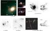 |
Fig. 1 a) RGB rendering of A68/C0 using the F160W, F814W, and F702W HST bands. Left: images A68-C0a and A68-C0b forming a broad quasi-symmetrical arc near the cluster BCG. Upper right: third, less magnified and less distorted image, A68-C0c. Lower right: source plane reconstruction of A68-C0c after removal of the overlapping elliptical. Some residuals of the subtraction remain. b) ACS/F814W image and source plane reconstruction of A68-HLS115. Again, the neighboring elliptical has been removed in the reconstruction. c) ACS/F814W image of A68-h7 with IRAC/ch2 contours. This source consists of an interacting system of four separate components, the most extinguished of which is the southwest component. Although the exact relation of each of the components to one another is unknown, their morphology and photometry is consistent with all of them being related and forming a coherent system. d) ACS/F814W image of A68-nn4 with IRAC/ch2 contours. This source consists of a pair of interacting galaxies. We focus on the northeast component as it is the most extinguished and appears to be the most related to the IR emission. e) Left: RGB rendering of the giant arc in MACSJ0451+0006 using the F140W, F814W, and F606W HST bands. The arc is 20′′ long, and can be separated in two main components: the northern part and the southern part. The northern arc is a double image of the northern part of the source. The critical line runs through the middle of it. The southern arc is a single stretched image of the rest of the source. The two parts can be separated in Herschel up to 250 μm. The IR emission in the south appears to be dominated by an AGN, so we consider here only the northern, and starburst component, of the IR emission. Right: ACS/F606W source plane reconstruction of the arc. The morphology suggests a merger, despite ambiguious kinematics (Jones et al. 2010). |
A68/C0: the C0 galaxy is a triple-imaged spiral galaxy lying behind the core of the massive galaxy cluster Abell 68. The two most magnified images (a & b) form a single continuous broad arc close to the brightest cluster galaxy (BCG). They are shown in Fig. 1. A third, less magnified and less distorted image (c) of this galaxy appears farther out on the opposite side of the BCG. This third image clearly shows the spiral nature of this galaxy. This galaxy was first reported by Smith et al. (2002a) from their search for gravitationally lensed Extremely Red Objects (EROs) and subsequently analyzed in more detail in Smith et al. (2002b). These initial papers focused on the bulge component of the galaxy. This part of the galaxy appears bright red in the composite JIR image shown in Fig. 1, and is the only readily visible component in the K band. In this paper, however, we always considered the galaxy in its entirety. By doing so, the galaxy no longer qualifies as an ERO. We performed our analysis only on the arc composed of images a & b, as these are the two brightest images, and because image c is blended with a cluster member elliptical galaxy. The combination of images a & b represents a linear magnification factor of μ = 30. The arc has also been referred to as the space invader galaxy, because of its appearance when looked at from the northwest1.
In our companion paper (Dessauges-Zavadsky et al., in prep.), we present CO observations of this arc, from which we infer a redshift of z = 1.5854. This redshift is consistent with the break detected by Smith et al. (2002b) in their z-band NIRSPEC spectrum and identified as the Balmer break. It also matches our detection of the Hα line in the NIR spectrum obtained with LBT/LUCIFER.
A68/h7: this source, also located in the field of the cluster Abell 68, consists of a system of four galaxies in interaction (Fig. 1). We obtained a VLT/FORS2 spectrum of this object from which we have identified faint C II and C IV lines and estimated its redshift to z = 2.15. We then confirmed the redshift with our CO observations (Dessauges-Zavadsky et al., in prep.). Although the FORS2 slit was positioned on the brightest (easternmost) component, the photometry and SED of all of the individual components is consistent with all of them lying at the same redshift. Furthermore, the CO spectrum shows only a single line of full width at half maximum FWHM = 350 km s-1. This strongly suggests that the four components are in some form of interaction, but the exact configuration thereof remains uncertain. It is possible, for example, that the system is made of a weakly interacting pair of two ongoing mergers.
A68/HLS115: the galaxy HLS115 is lensed by both the cluster itself and a cluster member elliptical galaxy for a total estimated magnification of μ = 15. We have detected Hα from this galaxy with LBT/LUCIFER, and CO with the IRAM/PdB interferometer (Dessauges-Zavadsky et al., in prep.), from which we infer a redshift of z = 1.5859. This redshift is nearly identical to that of A68/C0. The two galaxies, therefore, most likely belong to the same group. Contrary to A68-C0, however, HLS115 does not show a well-defined spiral structure, but instead consists of a series of clumps. It has, otherwise, very comparable properties as derived from our SED fitting (cf. Sect. 5).
A68/nn4: this source consists of a pair of objects in interaction. It has the highest redshift in the sample, z = 3.19. Here, we study the most obscured of the two components, which is also the one that appears to be the most related to the FIR emission. It is undetected from the R band and bluewards. This source lies in the outskirts of A68, so it is modestly lensed (μ ≈ 2.3), and thus intrinsically luminous.
MACS0451: this is a very elongated arc and highly magnified (μ ≈ 49) source at redshift z = 2.013 in the field of the cluster MACSJ0451.9+0006 (Jones et al. 2010). The arc measures 20′′ in length, and so this source is spatially resolved up to 250 μm. When examining the FIR SED of this source, we noticed differences between the northern and the southern parts of the arc, with the first peaking at 250 μm and the second at 100 μm, indicating very hot dust. After careful analysis of this object, we came to the conclusion that the infrared emission of this galaxy includes an AGN component. However, we are confident that we can separate this AGN component from the star-forming component. A detailed discussion will be presented in Zamojski et al. (in prep.). Therefore, we chose to retain this object in the current study given the rarity of such highly magnified objects at this redshift, but consider only its star-forming component. The contribution to the total IR luminosity coming from the two components is about half and half. The UV-to-NIR photometry has constant colors throughout the arc, with ~40% of the flux coming from the northern part. We see no signs of an AGN at these wavelengths. A decomposition of the IR emission of southern part of the arc indicates that roughly 55% of its flux originates from the AGN while the remaining 45% comes from star formation, the exact number depending on the models used. For simplicity, we employed here these round numbers as working values, that will be used in particular in Sect. 5.3, and postpone a more detailed analysis until later (Zamojski et al., in prep.).
We note that the detailed photometry of the arc presented here differs non-negligibly from previously published values (Richard et al. 2011). This difference stems from the different methods used to make these measurements. As explained in Sects. 2.2.1 through 2.2.3, we model the arc in its entirety starting from the high-resolution Hubble Space Telescope (HST) images and convolving with the proper point spread function (PSF), and then solving for the flux simultaneously with all neighbouring objects with a maximum likelihood algorithm. The flux thus extracted is robust. Previous values were extracted in a number of apertures along the arc with aperture corrections and color extrapolations applied to these measured fluxes. This approach is prone to larger uncertainties, and we estimate that the inferred factors of ~2−3 difference are not incompatible with these uncertainties. The arc possesses a dense photometric coverage in the optical regime coming from HST, the Subaru Telescope, and the Sloan Digital Sky Survey, with considerable overlap between the bands. Our method produces a smooth and consistent SED across these bands and across the different instruments, and the physical properties extracted from its SED are consistent with those obtained from other diagnostics (cf. Sect. 5.1.5). This would not otherwise be the case. It illustrates the difficulty of working with these highly stretched arcs and the importance of accurate photometry for proper modeling of their SED.
cB58 is a well-known very strongly lensed (Seitz et al. 1998, μ ~ 30) galaxy at z = 2.78 discovered by Yee et al. (1996). We use the Canada-France-Hawaii Telescope (CFHT) and Spitzer optical to mid-infrared (MIR) photometry provided by Ellingson et al. (1996) and Siana et al. (2008) together with the submm/mm detections of van der Werf et al. (2001) and Baker et al. (2001). Spectroscopy of this source is described in Pettini et al. (2000) and in Teplitz et al. (2000).
The Cosmic Eye: this is an equally strongly lensed Lyman break galaxy (LBG) at z = 3.07 discovered by Smail et al. (2007). It is magnified by a factor of μ = 28 ± 3 times by a foreground z = 0.37 cluster and a z = 0.73 massive early-type spiral galaxy (Dye et al. 2007). For our work we use the combined photometry of Coppin et al. (2007) and Siana et al. (2009). Spectroscopy of the rest-frame optical emission lines and the UV absorption features is available from Richard et al. (2011) and Quider et al. (2010), respectively.
2.1.2. Differential magnification
One caveat to working with strongly lensed galaxies is that some parts of the galaxy could be magnified more than others. This so-called differential magnification can modify the balance of the SED if the region being magnified more is particularly bright (or faint) at some wavelengths compared to the rest average of the galaxy, as would be the case for a particularly dusty region or cloud, for example. This could lead to erroneous conclusions when deriving global properties.
The advantage of working with cluster lenses (as opposed to galaxy lenses) is that they have much larger and broader potentials so that the magnification changes little on the scale of a galaxy. This, however, is true only as long as the source is not located near a caustic. Sources that cross inside the caustic region are imaged multiple times and could be prone to differential magnification effects. Within our sample, this happens with A68/C0 and the arc in MACS0451, as well as with our two comparisons objects: the Cosmic Eye and cB58.
The infrared emission of A68/C0 at 100 μm (highest resolution) is elongated and the ellipse covers well the visible part of the galaxy. This suggests that it originates from the entire disk rather than being dominated by a bright region near the critical line passing through the center of the object. Differential magnification does not appear to play an important role in this galaxy. The northern part of the arc in MACS0451 consists of two mirror images of the same part of the source, and is therefore also crossed by a critical line. The 100 μm emission, also in this case, does not appear to be any brighter near the critical line region. In addition, the region appears bluer than the rest of the galaxy in optical − IRAC colors, so that, again, the dusty and infrared-bright regions appear to be distributed, as is the optical/NIR light, throughout the whole image. The FIR emission does not appear to come from a small very magnified region near the critical line. The case for the Cosmic Eye and cB58 is more difficult, as we do not have the resolution to say anything about the spatial origin of their FIR emission. Differential magnification effects within these two galaxies cannot, therefore, be excluded.
2.2. Photometry
The data used in this study comes primarily from the Herschel, IRAC, and SCUBA2 Lensing Surveys (Egami et al. 2010; Smail et al. 2013, in prep.), as well as from ongoing efforts to image strong-lensing clusters with the HST. In addition, we collected data from various ground-based facilities to complement our wavelength coverage, and better constrain our stellar SEDs. The photometry for all sources is given in Tables A.1 and A.2.
2.2.1. HST photometry
Our sources are strongly lensed, and many of them appear close to large elliptical galaxies, such as the BCG, whose light blends with that of the objects we wanted to study. To obtain accurate photometric measurements, the light from these neighboring/lensing ellipticals needed to be removed. We did so by fitting their profile with GALFIT (Peng et al. 2002). A large dynamic range in terms of the brightness and extent of sources exists in the center of massive galaxy clusters, in addition to the high density of sources. It is, therefore, extremely difficult to fit the profile of all cluster galaxies simultaneously. We thus proceeded in steps, first by fitting and removing the light of the brightest galaxies, and then that of the more modest less extended objects2.
After subtraction of neighboring cluster galaxies, we use SExtractor (Bertin & Arnouts 1996) to measure the flux of our sources in elliptical apertures in a reference HST image. We extracted our objects in the reddest HST band available (usually F160W). In some cases (e.g., A68/C0, MACS0451), our sources are stretched so that they take the form of an arc, and ellipses no longer accurately represent their shape. For these objects, we employed custom apertures. We then measured the flux of our objects in other HST bands in those same apertures, after also performing a subtraction of neighbouring cluster galaxies in those bands.
2.2.2. IRAC photometry
Because of the much coarser resolution of the Spitzer Space Telescope compared to HST, we cannot employ the same strategy for IRAC images. Instead, we performed prior-based photometry. We adapted the code initially developed by Guillaume et al. (2006); Zamojski (2008); Llebaria et al. (2008); and Vibert et al. (2009) to do prior-based photometry for GALEX, and applied it to IRAC. Our code uses the Expectation Minimization algorithm, a Bayesian algorithm that iteratively adjusts the flux of all objects simultaneously in such a way as to increase, at each iteration, the likelihood that the observed image is drawn from the theoretical image: the theoretical image, in this case, being the image produced by convolving the prior shape of each object with the IRAC PSF and scaling it to the adjusted flux.
We used the reddest HST band to produce so-called stamp images of each object. These stamp images include only pixels within the SExtractor aperture. They define the prior shape of each object that is then convolved with the IRAC PSF and scaled in flux. For large elliptical galaxies whose profile include wide wings, we increased the size of the SExtractor aperture, often by a factor of ~2 or sometimes more, so as to include as much of the entire visible flux of the galaxy as possible, up to the surface brightness limit of our images. This was necessary because of the surface brightness depth of the IRAC observations. Had we not done this, we would not have subtracted these galaxies completely in IRAC, and hence we would not have measured their entire flux. More importantly, however, we could contaminate the flux of neighboring objects. The residual maps, in this case, would be dominated by the wings of these large galaxies hollowed out in their centers. We enlarged the apertures in order to avoid this.
There can be overlap between the ellipses of different objects. We deblended faint and background objects from cluster galaxies by extracting their shape and photometry from the image in which the profile of these cluster galaxies was removed as explained in Sect. 2.2.1. We then used the initial image to extract the shape of the larger galaxies, but only after first subtracting the flux of all the previously extracted fainter objects surrounding them. For cases where two or more similar size galaxies needed to be deblended from the same image, we employed the symmetric part of each galaxy, relative to their center, to deblend the flux in overlap regions as explained in Zamojski (2008) and Vibert et al. (2009).
Since the position and shape of our priors are fixed, and only their fluxes are adjusted, our method can naturally recover the flux of objects even when the fluxes of several objects partially overlap (separation ≳1 FWHM = 1.6″) as is the case of most IRAC sources in the crowded field of a massive galaxy cluster. After subtraction of the theoretical image from the actual image, some residuals can remain. These residuals are largest for resolved spiral galaxies, most likely because of the intrinsic differences in the shape of the galaxy at 1.6 μm and 3.6 μm, notably in the size of the bulge and the intensity of the spiral arms and star-forming clumps. Nevertheless, they remain on the order of ≲5%.
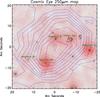 |
Fig. 2 HST/ACS image of the region around the Cosmic Eye overlaid with MIPS 24 μm emission in redscale and SPIRE 250 μm contours. Five objects, including the Cosmic Eye, blend to form a single source at 250 μm. Neighbor 4 is undetected in all of the optical bands, and faint at 24 μm, but appears in IRAC and shows up ever brighter with increasing wavelength in the infrared. Its SED indicates that it is probably an SMG an z ~ 2.5. |
2.2.3. Ground-based photometry
For ground-based images, we use both the procedure we apply to HST images and the prior-based method we use for IRAC, and retain the one that is most appropriate. In the case of strong blending with a neighbouring elliptical galaxy (such as for A68-HLS115), prior-based photometry is preferred, whereas for very extended objects (e.g. A68-C0) the combination of GALFIT and SExtractor or custom aperture is favored. In all cases, both methods give similar results.
2.2.4. IR-mm photometry: general
We used aperture photometry (with an appropriate aperture correction) on MIPS and PACS maps, since, at these wavelengths, our sources are well separated from other sources. Exceptionally, we used a SExtractor elliptical aperture for A68-C0 at 100 μm since the source is marginally resolved and elongated. In SPIRE sources begin to blend, so we used again our prior-based technique, this time with only the positions as priors with each object simply taking the shape of the SPIRE PSF. We retained as priors only those sources that are detected in at least one of the PACS bands.
In the case of the arc in MACS0451, we also used prior-based photometry on the PACS maps, since we wanted to separate the different components of the arc. We again trimmed our list of priors to avoid putting flux in unphysical places. Here, we simply removed, based on their color and shape, all low-redshift ellipticals, except for the BCG which may have contributed non-negligible flux to the IR (Rawle et al. 2012). Since the resolution of PACS is not as coarse as that of SPIRE, some sources can be marginally resolved (as is the case of A68-C0), and in particular the giant arc, even after splitting it into two or three components. However, optical/NIR images are hardly representative of the FIR morphology of a galaxy. We thus opted for the next best approximation and used exponential profiles as shapes for our priors, the effective radii of which are based on that of the optical/NIR light.
Except for A68-C0, our sources are faint, and detected at only a few sigmas, in the SCUBA2 maps. We therefore used prior-based photometry as it performs better than aperture photometry in terms of the depth at which it is able to measure fluxes, and of the reliability of the measurements, increased because the positions of the sources are known and fixed a priori. We used pure PSFs as shapes for our priors, and a circular Gaussian of FWHM = 14.5′′ to describe the SCUBA2 beam.
2.2.5. IR photometry: Cosmic Eye
The Cosmic Eye is surrounded by several other equally infrared-bright objects. Figure 2 shows the SPIRE 250 μm contours of the region around the Eye overlaid on top of an HST/ACS optical (F606W) image. Also overlaid on the same image is a MIPS 24 μm redscale, indicating four sources of infrared emission other than the Cosmic Eye within the same SPIRE resolution element. Neighbor 4 is undetected in any of the optical bands, but appears in IRAC. It is faint but detected in MIPS and PACS, and its SED indicates that it is probably an SMG at high redshift (z ~ 2.5). The most problematic, however, is Neighbor 1, as it is only 1 PSW pixel (6′′) away from the Cosmic Eye. In such heavily blended situations, even solutions obtained with PSF fitting can be quite degenerate and sensitive to the local noise as well as to initial prior inputs. In order to estimate the flux of the Cosmic Eye in the SPIRE 250 μm band, we therefore performed our extraction under several added constraints, which we discuss below.
Our strategy was to first extract the fluxes of all objects in the field up to the PACS 160 μm band, fit their SED, and extrapolate it to predict their flux at 250 μm. Because none of the sources are bright in the PACS bands, and because of the crowding in this area, the reliability of the aperture photometry, in terms of centering of the apertures as well as of contamination, is doubtful. In the case of the Cosmic Eye, we therefore chose to extract the PACS fluxes with our prior-based procedure using the MIPS 24 μm sources as priors. We performed MIPS 24 μm photometry in apertures.
We used archival HST and Spitzer/IRAC data to obtain multi-band optical/NIR photometry of the objects neighbouring the Cosmic Eye. We used this photometry to first fit for the redshift of the neighbours using only the stellar part of their SED3. We then fit a preliminary thermal SED, to the MIPS and PACS photometry only, by fixing the redshift to that obtained above. Using the best-fit SED, we obtained an initial guess of the flux at 250 μm, and ran our deblending algorithm with those initial guesses. Even then, however, the relative contribution of the Cosmic Eye and Neighbour 1 remains weakly constrained because of the small separation of these two objects. The maximum likelihood solution actually assigns more flux to the neighbour than to the Cosmic Eye. This is unlikely given their respective SEDs at λ < 250 μm. We, therefore, re-ran the procedure by first fixing the flux of Neighbor 1 to that predicted by the best-fit SED, subtracting it from the image, and removing it from the catalogue of priors. The new solution converges to fluxes for the Cosmic Eye and its three other neighbours close to those predicted by their preliminary SEDs. The residuals are slightly less flat than for the case where all five objects are free to vary, but they remain below the noise level. The difference between the two cases can therefore be said to be of little significance. We thus retained the second and more physical solution. The errors estimated from the residuals are added in quadrature to the dispersion of predicted fluxes for Neighbor 1 obtained with different libraries.
At 350 μm where the resolution is even worse than at 250 μm, the situation becomes even more degenerate, and we were unable to obtain a reliable measurement. We, therefore, chose to use only photometry up to 250 μm, in addition to upper limits at 350 μm, 500 μm, and 3.5 mm. We added, however, the 1.2 mm flux from Saintonge et al. (2013).
2.2.6. IR photometry: cB58
The source MS1512-cB58 is very close the cluster cD galaxy, which also shines in the infrared. Fortunately, its redshift is known spectroscopically to be z = 0.372. We can, therefore, extrapolate its flux at 250 μm and remove it from the image, before solving for the flux of cB58 itself, in exactly the same way as we proceeded to deblend the Cosmic Eye with its closest neighbour. cB58 is otherwise not as heavily blended as the Cosmic Eye, and we were able to obtain a reliable flux at 350 μm as well.
3. SED modeling
3.1. SED fits
We used an updated version of the Hyperz photometric redshift code of Bolzonella et al. (2000), modified to include the effects of nebular emission in its fitting procedure, as described in Schaerer & de Barros (2009, 2010). Designed to derive redshifts from broad-band SED fits of UV–NIR photometry and physical parameters of the galaxies, our version was also adapted to use data up to the submillimeter range. The redshift of our sources is fixed to the spectroscopic value and is not considered a free parameter in the present work.
Using the (semi-)empirical and theoretical templates described below, we perform fits of three sets of photometries per object:
-
the full photometry (i.e. from the rest-frame UV to the FIR);
-
the dust processed FIR emission (from the MIPS 24 μm band longwards);
-
the stellar SED photometry up to the IRAC bands.
These fits of different wavelength intervals are done to provide us with the widest range of parameters that can be deduced from the bulk spectral features of our sources as precisely as possible. They are described in detail in the following paragraphs.
Fits to the full photometry using empirical templates inform us whether the concerned object resembles a known local object or type. We perform fits to the full photometry only to inform ourselves whether the object in question resembles a known local galaxy or galaxy type. We do not use global fits to derive any physical quantity, as they typically reproduce poorly the observed photometry compared to the combination of the independent fits to the stellar and thermal components respectively. The only free parameter that Hyperz can explore for empirical templates is adding extinction on top of the original template used, if needed. This affects the template in the wavelength interval [912 Å−3 μm], where typically the light emitted by stars gets absorbed by the ISM. This increases the adaptability of the templates used, and comes in handy when exploring obscured IR-bright galaxies. Of course, the value of the extinction in this case is of no physical significance, since it does not consider the intrinsic extinction that comes with every original template. The total FIR luminosity LIR is obtained from integration over the rest-frame interval [8−1000] μm over the fits to the FIR only part of the SED.
We also performed modified blackbody (MBB) fits on the FIR/submm data to derive dust properties such as temperature and mass (see Sect. 6.6).
The full and FIR only fits are done using libraries whose templates are defined from the UV to submm wavelengths (typically they are defined from the Lyman limit to the synchrotron-dominated part of the electromagnetic spectrum). The libraries used are
-
Chary & Elbaz (2001, CE01): a set of synthetictemplates of varying IR luminosity;
-
Polletta et al. (2007, hereafter P07): a set of templates made up of local observed objects, including spiral galaxies, starbursts, Seyfert, and AGN, plus templates from synthetic models covering various stages of galaxy evolution;
-
Rieke et al. (2009, R09): a set of templates containing observed SEDs of local purely star-forming LIRGs and ULIRGs, and some models obtained as the result of combining the first ones. These templates in particular are defined only down to 3 μm or 4000 Å and hence are only considered for the FIR only fits;
-
Michałowski et al. (2010, M10): a set of templates made from observations of submm galaxies at z ~ 0.08−3.6 (Hainline et al. 2009, 2010).
For every set, a free scaling parameter allows matching in terms of intensity.
Various combinations of the basic parameters that we explore in our stellar models.
The fits to the stellar SED determine the physical parameters such as the SFR, stellar mass, age of the population, the extinction AV. From the fitted SED we also derive the UV slope β4, and UV luminosity LUV5. They are performed with the Bruzual & Charlot (2003) library (BC03 hereafter). We adopt a Salpeter IMF from 0.1 to 100 M⊙. The extinction laws explored here are the commonly used Calzetti law (Calzetti et al. 2000) and the SMC law of Prevot et al. (1984), motivated also by recent publications (Reddy et al. 2012b; Oesch et al. 2013; Wuyts et al. 2012). When there was available spectroscopic data for comparison, we also explored Calzetti’s law with stronger line attenuation as prescribed in Calzetti (2001) (in particular in the case of the Cosmic Eye).
From the fits to the SED, assuming energy conservation, we also derive the predicted IR luminosity from the difference between the intrinsic, unobscured SED and the observed IR luminosity, as described in Schaerer et al. (2013). Having access to the actual observed IR luminosity allows us to distinguish/constrain different SFHs and extinction laws.
For the BC03 library, and following our analysis of a large sample of LBGs from redshift 3 to 6 (de Barros et al. 2012; Schaerer et al. 2013), we explore a range of SFHs, as well as models with or without nebular emission. Except otherwise stated, we assume solar metallicity. The combination of model parameters explored is summarized in Table 2. In practice we have used SFHs with exponentially declining timescales with τ = (0.05,0.07,0.1,0.3,0.5,0.7,1.,3.) Gyr, exponentially rising ones with τ = (0.01,0.03,0.05,0.07,0.1, 0.3,0.5,0.7,1.,2.,3.) Gyr, or constant SFR with a minimum age prior of tmin = 100 Myr, as commonly assumed in the literature. The extinction is allowed to vary from AV = 0 to 4 in steps of 0.1. We also apply a foreground galactic reddening correction to our photometry, using the values available from the NED (Schlegel et al. 1998).
The ratio of LIR over LUV is known to be an effective tracer of UV attenuation (e.g. Burgarella et al. 2005a; Buat et al. 2010; Heinis et al. 2013). From the observed LIR/LUV we can therefore determine the extinction needed in Hyperz to make fits that are energy conserving, meaning that the stellar population model produced in this case will reproduce the actual observed LIR without suffering from the eventual age-extinction degeneracy often encountered in obscured galaxies. In practice, we use the relation between LIR/LUV and AV from Schaerer et al. (2013). These “energy conserving models” should thus provide the most accurate physical parameters.
For each object we retain the best-fit SED and physical parameters. We also generate 1000 Monte Carlo (MC) realizations of the observed SED, which are fit and used to determine the median values and the 68% confidence intervals of the various physical parameters. Although the photometry’s precision is better for some observed bands, we have imposed a minimal error of 0.1 mag (and 0.05 mag for MACS0451 that has overall very well constrained photometry) in the SED fitting procedure and the MC catalogs that is more appropriate when combining the photometry from many different instruments, wavelengths, and depths.
Main observed and derived properties of our galaxies.
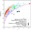 |
Fig. 3 IR luminosity of Herschel-detected galaxies as a function of redshift showing the position of our five lensed galaxies (open diamonds), two well-studied lensed galaxies from the literature (cB58 and the Cosmic Eye, marked as grey diamonds), and galaxies from various blank field observations, including data from the GOODS and COSMOS blank fields by Symeonidis et al. (2013) and Elbaz et al. (2011). Also plotted is the SMG sample of Magnelli et al. (2012a), and the hyLIRG detected by the HLS behind Abell 773 (Combes et al. 2012). Clearly, most of the lensed galaxies at z ~ 1.5−3 extend the blank field studies to fainter luminosities into the LIRG regime. The typical uncertainty of our LIR measurements is ± 0.1 dex or smaller. The red curve shows the minimal LIR at each redshift that can produce a flux ≥2 mJy in PACS160 (2× the confusion limit, ~3σ detection limit in GOODS-N). |
4. IR properties of the sample
The main observed quantities of our sample, derived from simple SED fits, are summarized in Table 3. The SPIRE and PACS data provide good constraints on the dust emission peak, allowing us to evaluate precisely the FIR luminosity LIR determined from integration of the best fit SED in the wavelength interval [8,1000] μm. Fits with the different libraries we used typically agree within 0.05 dex when they accurately reproduce the photometry. A comparison with the code Cmcirsed of Casey (2012) yields a mean ⟨log (LIR(CMCIRSED)) − log (LIR(Hyperz))⟩ = 0.016 ± 0.079, showing no systematic offset. Best-fit SEDs are shown and discussed below. Based on these values and correcting for the lensing magnification factor μ, we then calculated the IR inferred SFRs, SFRIR, adopting the Kennicutt (1998) calibration. The temperature Tdust, a measure of the dust temperature, was derived by fitting modified blackbodies to the FIR/submm data using an emissivity index of β = 1.5. Further discussion on the values and parameters used can be found in Sect. 6.6.
Overall, the observed IR luminosities of our objects are in the range (3−16) × 1012L⊙. However, the intrinsic, lensing-corrected values are considerably lower, between 6 × 10¹⁰ and 6 × 10¹²L⊙. The intrinsic IR luminosities of our sample are shown in Fig. 3 as a function of redshift, and are compared to other galaxy samples observed with Herschel. Clearly, our sample extends previous blank field studies to lower LIR magnitudes, thanks to gravitational lensing.
In our comparison sample, we note that the inferred IR luminosity of the Cosmic Eye, log (LIR , is ~0.3 dex lower than the estimated value in Siana et al. (2009), about ~0.05 dex below their quoted 1σ interval, which was determined in the absence of Herschel data. Our measure is in exact agreement with the estimation of Coppin et al. (2007) based on the rest-frame 8 μm flux.
For cB58 our IR luminosity, determined from the available FIR measurements (with new PACS and SPIRE data added to the existing MIPS and 850 μm and 1.2 mm), is log (LIR·μ) = 12.96 ± 0.01, which is notably brighter than the 12.58 ± 0.08 derived by Wuyts et al. (2012) and the earlier estimate of 12.48−12.78 from Siana et al. (2008). This is mainly because of the detection of a warmer dust temperature made accessible by the Herschel observations (and is discussed further in Sect. 6.6).
The recent publication of Saintonge et al. (2013) has cB58 and the Cosmic Eye in common in a similar analysis of their IR emission. We find the same LIR for cB58 within our margin of errors. Our estimation of the LIR of the Eye is ~0.2 dex lower than theirs. This is because of our de-blending work (see Sect. 2.2.5) that lowered the fluxes attributed to this particular source.
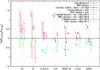 |
Fig. 4 Predicted over observed ratio for LIR for all the galaxies modeled and for the different stellar population scenarios we have explored (dashed symbols stand for declining SFH models including nebular emission, solid lines neglecting this effect, dot-dashed cyan and magenta consider rising SFH scenarios including nebular emission). We can see that the SMC-based predictions underpredict LIR in almost all cases. The Calzetti-based models, although more degenerate, achieve a match with most of the objects’ observed LIRwithin the 68% confidence range. The rising SFH models predict globally at least as much or more LIR than their corresponding (in terms of extinction law) declining SFH ones (as shown in Schaerer et al. 2013), pushing in particular the Calzetti-based models to overpredict the observed quantities. The effect is similar but smaller for the SMC-based solutions, and allows a perfect match in the case of C0. We note that for MACS0451N the observed LIR of the northern part, representing ~1/3 of the total, was adopted here and the predicted LIR compared here are also derived for this same region, for coherence. This means that, depending on the model, the predicted LIR used are ~35−40% of the values listed in Tables 4 and 5. If one plotted the same for the total arc in the eventuality of a negligible AGN contribution the ratios shown would be scaled down by ~0.15 dex at most. |
5. SED fitting results
5.1. Results for individual HLS galaxies
We now present and discuss the detailed results from the SED fits for each galaxy and the differences obtained for models using different SFHs and extinction laws, with or without nebular emission. The main derived physical parameters are summarized in Table 4 for variable SFHs, and in Table 5 for classical models assuming constant SFR and neglecting nebular emission. We present in some cases more than one of the different solutions obtained, regardless of the reduced  values (almost all of our solutions are in very good agreement with the photometry), where we deem a discussion interesting when comparing the physical interpretation of our objects with the different models used. The energy-conserving models with fixed extinction are discussed separately, after the discussion of the individual sources, in Sect. 5.3. The physical parameters are discussed and compared to other samples in Sect. 6.4. The IR luminosities predicted from the various SED fits are compared to the observed LIR in Fig. 4. This comparison provides a consistency check on the dust extinction and on the age and SFH-dependent luminosity emitted by the stellar population.
The different sizes of the error bars seen are mainly due to different numbers of free parameters. The constant SFR scenario has the smallest number of free parameters (it allows only constant SFR and also forbids ages below 100 Myr, which does not leave room for much degeneracy). The other cases allow varying timescales in star formation (as stated in Sect. 3.1). Only the declining SFH models using Calzetti’s law are really prone to the age-extinction degeneracy. SMC-based models tend to favor long timescale scenarios, and the rising SFH models converge regardless of timescale as they must be at peak star formation at age t, and thus will tend to have the same extinction to reproduce the SED’s colors. After a case-by-case discussion we will come back to this in Sect. 6.1.
The following subsections are organized in a standard pattern, with two main paragraphs each, a first one discussing the stellar models, and the second the FIR fits. In particular, we discuss how the physical parameters depend on the model assumptions (mostly SFH and extinction law) and we examine how the FIR data allow some of the assumptions to be ruled out.
Selected variable SFH models, with physical properties derived from fitting with the BC03 library.
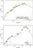 |
Fig. 5 Top: SED plots for A68/C0’s best stellar population fits using the two extinction laws. In the case of Calzetti, the fit including nebular emission was prefered. Bottom: global and FIR-only fits. The best fit for the full photometry uses a Seyfert galaxy template from P07 (shown in red) and an extra extinction of AV = 0.6 by the SMC law. The FIR only SED (in green) is by R09. |
5.1.1. A68/C0
The SED fits of A68/C0 performed on the visible to NIR photometry can be seen in Fig. 5, and show the best solution for Calzetti, and the best one for SMC. In terms of the overall best fit was obtained with the Calzetti-based, declining SFR (τ = 300 Myr) model that includes nebular emission. It interprets C0 as an obscured (AV = 1.7) population involving a starburst/post-starburst in a moderatly young age, t = 180 Myrs, with a well-sustained SFRBC(t)/μ of ~36 M⊙ yr-1 (see Table 4 for error estimates). The important extinction overpredicts the observed FIR luminosity by a factor of 4 for the best fit, and  for the MC runs, which puts it on the edge of the derived 68% confidence interval, as shown in Fig. 4. A similar discrepancy is also found with standard SED fits assuming SFR = const. and neglecting nebular emission.
Fits with the SMC law has only a slightly larger  , but give a significantly different interpretation that agrees better with the idea that C0 is a quiescently star-forming galaxy, it has a very old population of t = 3.5 Gyr, and an almost constant SFH (τ = 3 Gyr) with SFRBC(t)/μ ~ 10 M⊙ yr-1. In this case the extinction is AV = 0.5, and the predicted IR luminosity has its upper 68% limit slightly below the observed LIR (cf. Fig. 4), but matches it at 90%. Perhaps a special mention can be made for the SMC-based rising SFR model, as it reproduces almost perfectly the observed LIR (and A68/C0 is the only case where this happens in our sample). This model actually resembles in most aspects the one just described, with the same age (oldest allowed at this redshift) and very slowly increasing SFR (same τ = 3 Gyr, largest among our rising SFHs), and SFRBC(t)/μ ~ 18 M⊙ yr-1, hence a slightly higher extinction allowing the correct prediction of LIR. Based on this model and the IR observation, the quiescently star-forming galaxy scenario seems well suited, only with more current SFR than in the past, rather than the opposite.
Despite these differences, the stellar mass of A68/C0, M⋆ ≈ (2−4) × 1010M⊙, agrees within a factor of ~2 for all models.
The best full SED fit, shown in Fig. 5, was obtained with templates from the P07 library, with some further extinction by the SMC law. Its steeper slope in the UV allowed for a better match of the B-band’s photometry (rest-frame UV) without reddening the SED enough to degrade the fit in the rest-frame optical. The fits show a slight underestimation of the dust emission peak, but is in agreement with the [8−1000 μm] IR luminosity, found to be log [LIR/L⊙] = 12.55 ± 0.03. The interpretation of the templates’s dust emission peak gives a dust temperature of ~35 K using Wien’s displacement law. The de-lensed SFRIR is ≈20 M⊙ yr-1, using the Kennicutt (1998) calibration. The SMC-based models that favored long, almost constant SFHs are slightly beneath this value, as is their predicted LIR. Models with the Calzetti attenuation law overpredict LIR by a factor of ~2.5 but marginally reproduce it within their 68% confidence level (cf. Fig. 4).
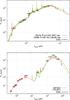 |
Fig. 6 Top: A68/h7 stellar population fits including nebular emission. Here the older Calzetti-based population renders the photometry longwards of 4000 Å well, but fits less the UV, and ultimately the SMC has the smallest |

5.1.2. A68/h7
The A68/h7 source shows a very red slope in its photometry and is peculiarly prone to a large degeneracy in terms of age and extinction. Naturally, this translates to large uncertainties in the expected IR emission, as can be seen in Fig. 4. The best fits are obtained without nebular emission regardless of the extinction law, and the SMC-based model produces ultimately the smallest . The SMC-based solutions favor slowly decaying almost constant SFHs when excluding line emission, and do not seem to favor any particular SFH when including it. Instead, the Calzetti-based models favor very rapidly declining SFHs (τ = 50 Myr, the smallest rate in our parameter space) for the runs that include nebular emission, whereas the SF timescale is less well constrained without lines. In all cases, the inclusion of nebular emission degrades the fit quality by a factor of 1.5−1.6 in terms of , which is not very important, but as we can see in the following, it affects very strongly the physical interpretation for the Calzetti-based models. Best-fit SEDs to the stellar part of the SED are shown in Fig. 6. Although differing by a factor of ~2 in , the two fits that show different extinction laws are clearly fairly similar, and satisfactory. It can also be seen that for the case of this obscured/old population the emission lines are not very strong, which is logical.
How does the inclusion of nebular emission affect the assessment of physical parameters? For the SMC law the changes are small. However, with the Calzetti attenuation law, there is a strong divergence in the solutions, with the one including nebular emission shifting the median age from 10 Myr to 360 Myr6. The solution without nebular emission seems highly unrealistic, as it has a median solution for SFRBC/μ that is ~8000 M⊙ yr-1, and spans at the 1σ level from ~3 M⊙ yr-1up to ~16 000 M⊙ yr-1. So actually the model including lines lies within a subregion of the whole degenerated parameter space of the former. In addition, in terms of extinction the model without lines has its 1σ interval for AV between 0.3 and 2.8, whereas for the model with nebular emission the derived AV range (between 0.2 and 1.4) is less extreme. Despite the differences between the models just discussed, the stellar mass agrees quite well (within ~20%) for the models listed in Tables 4 and 5.
The full and FIR SEDs of A68/h7 can be seen in Fig. 6. The full SED fit was obtained with an SMG template from M10, with additional extinction on the rest-frame UV/optical slope. An AV of 0.5 with the SMC law yields a that is ~3 times smaller than with the Calzetti law, which is driven by the steep UV slope given by the photometry. The best fit of the FIR data was obtained with the Rieke templates and gives a lensing corrected LIR of  . The highly degenerated solution for the Calzetti models makes it hard to produce a robust statement about how their LIR predictions can help us consider these SFHs to be accurate. In particular, the solution without nebular emission which spans across ~2.5 dex at the 1σ level actually contains every variant between an extreme young/obscure starburst to a quiescent/old population (cf. Fig. 4). As already discussed, the addition of line emission reduces in this case the degeneration towards the older solution which still predicts the observed LIR within 1σ. The SMC-based predictions fall short of the observed LIR at 3σ regardless of line emission, which indicates solutions that are probably slightly too old. Clearly, the standard model SFR, SFRBC, derived for SED fits assuming constant SFR, is inconsistent (too large) with the SFRIR derived the standard calibration. This, and the large degeneracies found for the fits of this object, shows that the instantaneous SFR of this galaxy cannot accurately be determined with the current approach. As we will see with the energy conservation approach discussed in Sect. 5.3, the use of the observed LIR as a constraint in our population modeling proves to be a very useful tool in breaking these degeneracies.
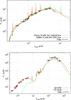 |
Fig. 7 Top: A68/HLS115 stellar population SEDs. The Calzetti-based model with nebular emission (green) is plotted together with the SMC-based model (red) for comparison. Although formally the best |
5.1.3. A68/HLS115
The SED of HLS115, shown in Fig. 7, is very similar to that of A68/h7, with a slope almost as red. The model based on Calzetti’s law, exponentially declining SFR (τ = 50 Myr), and nebular emission is still a very good fit and also manages to reproduce LIR within a rather narrow uncertainty interval. The SMC-based solutions not only produce fits of lower quality in this case, but they also predict an insufficient IR luminosity.
The physical properties of HLS115 with the aforementioned model (see Table 4) describe it as a young galaxy that has passed through a recent starburst. With M⋆ ≈ (0.7−1.5) × 1010M⊙, AV ≈ 1.5−1.9, and t ≈ 50−130 Myr it still actively forms stars at SFRBC(t) ≈ 30−100 M⊙ yr-1(at a 68% confidence level). Considering the two models listed in Table 4, the median stellar mass differs by a factor of three, mostly because of age differences.
The best fit for the UV-to-FIR photometry was again obtained with a M10 template (see Fig. 7). It reproduces well the stellar emission with an additional extinction of AV = 1.2 with Calzetti’s law, but misses the IR peak by a factor of ~1.5. The FIR photometry is best fitted by a template from CE01, and gives a lensing-corrected LIR ≈ 3 × 10¹¹ L⊙. This corresponds to a SFRIR of ~51 M⊙ yr-1 with the Kennicutt (1998) calibration, well within the 68% confidence intervals produced by the stellar population fit. As already mentioned above, the IR luminosity is well predicted by the Calzetti-based models, and, as already seen for the other objects, including nebular emission reduces the degeneracy/uncertainty (as shown in Fig. 4). The restricted scenario based on Calzetti, CSFR, and tmin = 100 Myr, yields similar results. As can be noted, A68/HLS115 is a clear case where the predicted IR emission allows the SMC extinction law to be excluded.
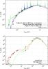 |
Fig. 8 Top: SED plot for the A68/nn4 stellar population with non-detections shown by 1σ upper limits. For such a strongly obscured galaxy, the two extinction laws produce quite different slopes, with the Calzetti law being unable to reproduce the steep photometry at the 1σ level. Allowing for more extinction (AV ≥ 4) could not offer a better fit since this law is relatively flat, and it would have worsen the minimization in the rest-frame optical domain. The SMCibased solution, on the other hand, is steep enough. The nebular lines are relatively weak, since despite the very young age they are also absorbed, and have little effect on the solution here. Bottom: full SED fit (red), obtained with the template of IRAS 20551-4250 from the P07 library, with an additional SMC-based extinction of AV = 0.4. Given the intrinsic attenuation of the template and its characteristic 2175 Å bump, adding more extinction in order to pass beneath the 1σ-detection limits was not possible. The best fit of the FIR data (green) was obtained with the CE01 library. |
5.1.4. A68/nn4
As mentioned in Sect. 2.1.1, we study here the faintest and reddest component of what seems to be a pair of galaxies in strong interaction. Its UV slope is so steep that no fits were successful when using Calzetti’s law, at least at the 1σ level. In Fig. 8 we show a plot comparing the two solutions with and without nebular emission for the SMC-based models, plus the Calzetti-based solution including nebular emission for comparison. The photometry is very well fitted without emission lines ( = 0.85), and the fit is somewhat degraded when adding them ( = 2.7), although it is mostly the flux in the K-band that gets overestimated because of the [O iii] λλ4959,5007 lines. In both cases the models produced describe a powerful (de-magnified SFRBC ~ 1200 M⊙ yr-1) and very obscured (AV ~ 1.9 for the SMC law) starburst at a young age; t ≈ 30 − 40 Myr is indeed the youngest age we haveve seen in the sample for a SMC-based model. The addition of lines downscales slightly the continuum and the physical quantities, and pushes the age towards ~60 Myr. The Calzetti-based model with no emission produces an extreme solution with a median age of 2.5 Myr, AV ≈ 3.9−4, and a de-magnified SFRBC above 105M⊙ yr-1! This solution is very unlikely, but it is interesting to see here again that the effects of adding nebular emission to the model reduces slightly its extreme character, and produces a solution with t ≈ 13−18 Myr, AV ≈ 2.2−2.9, and SFRBC ≈ 300−3000 M⊙ yr-1. The solution here is more degenerated, but falls within reasonable orders of magnitudes, also for the predicted IR luminosity, as can be seen from Fig. 4. This said, we can see in Fig. 8 that the spectral slopes produced with this solution are rather different than with the SMC-based solution, and fall short of the 1σ error bars. The Calzetti-based solution with higher line attenuation (E(B − V)⋆ = 0.44 × E(B − V)neb) gives a solution that lies between the one for E(B − V)⋆ = E(B − V)neb and the one excluding line emission, both in terms of and in terms of derived properties. The predicted median masses differ by a factor of ~4 between the different fits, with more plausible values probably being on the high side, M⋆ ≈ 2 × 10¹¹M⊙, corresponding also to a more realistic typical age for such an IR-bright galaxy.
The best fit for the whole photometry was obtained with the template of IRAS 20551-4250, a local merger and a ULIRG from the P07 library, with an additional SMC-based extinction of AV = 0.4 (Fig. 8). The extreme attenuation in the rest-frame UV range could not be reproduced without damaging the fit redwards, but most of the photometry is correctly matched at a ~2σ level, with the dust peak only slightly colder than what we can see in the FIR only fit. Given the low gravitational magnification (μ = 2.3), its intrinsic luminosity is very high, making it the brightest in our sample, a ULIRG with LIR≈ 6 × 10¹² L⊙. This luminosity is very well reproduced by the SMC-based model with no lines, with very little spread at the 1σ level (see Fig. 4). When adding line emission here, the general downsizing of the solution makes it miss the observed LIR by a little, and is a bit more degenerate. For the Calzetti attenuation law, we can see that line emission also has the same drastic effect of reducing the LIR, bringing it from a highly overestimated value (>1 dex) to within acceptable agreement with the observed value. Standard fits with constant SFR and neglecting nebular emission also predict LIR correctly, although they fit the stellar part of the SED less well. As expected, this fit also yields an SFRBC ≈ 880 M⊙ yr-1 in close agreement with SFRIR. This galaxy has also the warmest dust peak in our sample with Tdust ≈ 55 K.
5.1.5. MACS0451 Arc
This galaxy is a peculiar case and will be discussed in detail in Zamojski et al. (2013, in prep.). Here we will only describe its stellar population modeling, and some of the derived properties. We note that the UV-to-NIR SEDs were obtained by using the integrated photometry of the whole arc, which presented the same colors throughout its length. If one were interested in the quantities of the northern part only, the correction factor would be about ~0.4.
The stellar SED of this arc can be seen in Fig. 9. It is a clear case of how the inclusion of nebular emission can successfully fit some photometric points (here F140W) that otherwise could have led to photometric redshift misinterpretations in the absence of spectroscopic data. The F140W band presents an excess for any stellar continuum emission modeled to fit the whole set, but falls on the [O iii] λλ4959,5007 and Hβ region, and we see that this strong emission lines can account for the ~14% of missing flux, thus improving the by a factor of ~5. The physical properties all tend towards a very young age ≈15 Myr and a very low stellar mass M⋆ ≈ 1.5 × 10⁹M⊙. The very blue slope (the bluest in the sample) is probably dominated by very young stars. These aspects give an instantaneous SFRBC of ~100 M⊙ yr-1which, combined with the very young age, shows that our model interprets the photometry as a starburst. When using the classic model with tmin = 100 Myr, we obtain a constant SFRBC of ~34 M⊙ yr-1 and a mass approximately three times higher (M⋆ ≈ 5 × 10⁹M⊙). Since the predicted IR luminosity is quite close to the observed, this SFR value also lies within the limits of the SFRIR ~ 15−42 M⊙ yr-1, where the lower (higher) value comes from the LIR of the northern part (total) of the arc. The model that produces the smallest instantaneous SFR is the SMC-based one, which models the colors around the F140W band with a larger Balmer break and nebular emission, and achieves an age of 720 Myr and SFRBC ~ 13 M⊙ yr-1. The downside of this scenario is that it requires too little dust extinction to fit the data, thus strongly underpredicting the observed LIR. The stellar mass in this scenario is ~4 times larger than for the Calzetti-based one, but still about a factor of 2 less than the one estimated in Richard et al. (2011), probably because of a strong overestimation of the IRAC photometry in their work. Given the uncertainty on LIR owing to the possible presence of an AGN in this galaxy, this object is not well suited to obtaining good constraints on the SFH.
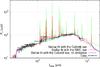 |
Fig. 9 Stellar SED plot for the MACS0451 arc. Note that the F140W photometic point can only get well fitted with the help of nebular emission in the case of Calzetti’s law (green). When using the SMC law (red), this flux is matched by the combination of a Balmer break and the line emission, but the χ2 is slightly larger than the Calzetti solution. The blue curve shows that fits without nebular emission can not produce enough flux to match the F140W point. |
5.2. Other lensed galaxies
To extend our sample of lensed galaxies, for comparison with other studies in the literature, and to test in particular the strength of the emission lines predicted by our models against spectroscopic observations available for these objects, we have also modeled in detail cB58 and the Cosmic Eye two well-know galaxies at z ~ 2.7−3.1. Once the available (broad-band) photometry of the stellar part of the SED is fitted, our models still predict the IR luminosity and the strength of numerous emission lines, which are not included as a constraint in the fitting procedure. They thus represent very useful a posteriori tests/constraints of the models, as discussed in Schaerer et al. (2013).
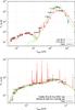 |
Fig. 10 Top: observed and model SED for cB58. Although not a good fit, the best match to the full, global SED is found with templates from M10. We can see that the template does not match the photometry in the NUV-blue as it does not describe a population as young as is cB58’s and misses the IR peak by a factor of ~2.5. The FIR fit is obtained with a template among the brightest and warmest from CE01 that matches the IR peak very well. Bottom: SED fits to the stellar part of cB58. The red line shows the best-fit for declining SFHs, including nebular emission, and assuming the SMC extinction law. Green shows the fit neglecting nebular emission and assuming the Calzetti law (best fit among the Calzetti-based solutions). We can see that for the Calzetti law the fitted SED falls out of the 1σ uncertainty of the g-band photometry as noticed in Wuyts et al. (2012) and Siana et al. (2008). In this a case, UV slopes derived from SED fits can vary substantially depending on the extinction law used, especially around the 1300−1800 Å interval. |
5.2.1. MS1512-cB58
The global SED of cB58 from the optical to the submm domain is shown in Fig. 10. The best fit was obtained using an SMG template of M10, which still shows some significant deviations from the observations: the Balmer break is much stronger in the template, and it fails to reproduce the intensity and steepness of the FIR emission, as is usually seen with IR-bright galaxies. The FIR-only best fit is also achieved with one of the brightest templates from CE01, which successfully reproduces the fluxes from 70 μm to 850 μm, with only a slight overestimation of the 1.2 mm band. The rather poor fit of the MIR photometry can be explained by the weak PAH features of the bright end of the CE01 library. This fit, including the new Herschel observations of cB58, provides the slightly revised lensing-corrected IR luminosity LIR = 3.04 × 10¹¹L⊙ listed in Table 3.
Fits to the stellar part of the SED (i.e. up to 8 μm) are generally good, independent of the detailed model assumptions (SFH and extinction law), and with or without nebular emission. Two examples, here assuming different extinction laws, are shown in Fig. 10. The strongest emission lines, [O ii] λ3727, [O iii] λλ4959,5007, and Hα, lie outside the observed bands, so they cannot contribute significantly to the photometry. However, the [S iii] λλ9069,9532 lines lie in the IRAC 3.6 μm band, where they can slightly contribute to the observed flux.
As seen with Wuyts et al. (2012) and Siana et al. (2008), the rest-frame UV photometry is best fitted with the SMC law, mainly thanks to its steepness in the FUV regime, that better accounts for the g − V and V − R colors. In this case, the usual power law approximation for the UV continuum becomes very ill-defined, unless one can distinguish a redder FUV regime and a bluer NUV one. Nonetheless, the mean slope we measure from our SEDs at 2000 Å β = −1.15 ± 0.1 is in very good agreement with the photometry in the VRI bands and the spectroscopic value of −1.28 ± 0.14 from Baker et al. (2001).
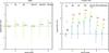 |
Fig. 11 Left: comparison of additional observables with model predictions for cB58 adopting the Calzetti attenuation law. Shown is the logarithmic ratio of the model prediction with respect to the observable quantity for LIR, the flux in the Hα, Hβ, [O ii] λ3727, and [O iii] λλ4959,5007 lines, as well as the Hα equivalent width. The observed values are from this paper (LIR), and from Teplitz et al. (2000). Although other emission lines have been detected in this galaxy, we do not include them here because the information they provide is basically redundant. Error bars indicate the 68% confidence interval predicted by the models; the typical observational errors, not included here, are shown with the black dotted error bars. Colors correspond to models with different SFHs (green: exponentially declining, and yellow: delayed SFHs; both for subsolar metallicity, 1/5 Z⊙. Black: SFR = const.; red: exponentially rising; both for solar metallicity). Results for the SMC law are similar and equally reproduce the observables. Right: same as left panel for the Cosmic Eye adopting the Calzetti attenuation law. Sources of the observational data are described in the text. Blue points show the predictions for models with exponentially declining SFHs and higher extinction to nebular emission (i.e. E(B − V)⋆ = 0.44 × E(B − V)neb). Red and black dashed symbols show the same for the rising and constant SFR models, respectively. |
Since other observables (lines and IR luminosity) have also been measured for this galaxy, it is interesting to compare them with the predictions from our models. This comparison is shown in Fig. 11 for the additional key observables, not included in the SED fits. Again, we note that all models are able to reproduce the observed IR luminosity and the main emission lines within a factor of few, typically two. Constant SFR models and rising SFHs predict emission lines that are slightly too strong, but applying a different (i.e., stronger) attenuation to the nebular spectrum compared to the continuum (as observed in nearby starburst galaxies in Calzetti et al. 2000) would reduce this difference. We note that here we have shown the results allowing for different metallicities (solar and 1/5 Z⊙), bracketing the range of the observed metallicity of cB58 of 1/3 Z⊙ (Teplitz et al. 2000), and adjusted to show the best results for each SFH. As expected, for SFHs allowing for strong variations (declining or delayed SFHs) the range of predicted line strengths is larger. Overall we conclude that the observations of cB58 do not provide a strong test/constraint for the SFHs and attenuation laws applicable to this galaxy.
The physical properties derived from a subset of models are summarized in Table 4. Typically, the median mass is M⋆ ≈ 6.5 × 10⁹M⊙, the instantaneous SFR ≈ 13−66 M⊙ yr-1, the extinction AV ≈ 0.3 − 0.9, with uncertainties of a factor of ~2. Ages (defined as time since the onset of star formation) are 30−60 Myr for declining SFHs, 50−90 Myr for delayed SFH, and older (100−250 Myr) for constant SFR or rising SFHs. No systematic age shift is found between the two attenuation laws considered.
The physical parameters derived here are very similar to those derived by Wuyts et al. (2012) when accounting for the normalization factor of 1.7 due to different the IMFs used between the two works7. We note that the stellar mass derived by Siana et al. (2008), a factor of ~5 lower than our value, is affected by an error in their SED scaling (Siana 2012, priv. comm.). Our SFR determination is also in good agreement with the SFRIR + SFRUV = 52.5 ± 10 M⊙ yr-1 obtained from the observed UV and IR luminosities (Table 3)8. Our values are in good agreement with the Wuyts et al. (2012) SMC-based SFR(SED) and with the Siana et al. (2008) LMC-based SFR(SED) and their SFRIR + SFRUV. From their SED fits using the Calzetti law, Wuyts et al. (2012) find SFR(SED) systematically larger than other SFR indicators, including SFR(Hα), which they and earlier studies (cf. Reddy et al. 2012b; Siana et al. 2009) consider to be an incompatibility, suggesting a preference for the SMC extinction law. The fair agreement of most/all of our models with the observed IR luminosity and the Hα flux demonstrates that there is no such inconsistency. Apparent differences between the various SFR indicators can naturally be explained by simplifying assumptions mostly on age and SF timescale made for these calibrations, as discussed in depth by Schaerer et al. (2013). Although formally the best fit is found for the SMC attenuation law, the observations of cB58 do not allow one to draw firm conclusions on the favored extinction law for this galaxy. The main signal leading to a slight improvement for an extinction law steeper than Calzetti is the photometry in the g-band filter, as already shown in Siana et al. (2008).
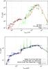 |
Fig. 12 Top: observed and model SEDs of the Cosmic Eye. The global SED is obtained with a Seyfert galaxy template from P07 but is a very poor fit, although it is the best fit among our libraries (an SMG template from M10 manages a better fit of the visible-NIR photometry, but misses the FIR data by more than one order of magnitude). The FIR data are best fitted by a R09 template, that accurately matches the photometry and 1σ limits, only slightly over-estimating the 1.2 mm detection. Bottom: comparison of the Eye’s best Calzetti fits with and without emission lines to the stellar SED. Also plotted is the very old (~1.5 Gyr) SMC-based model, which despite its large age, has favored a constant SFR and produces stronger lines than the Calzetti-based model. The difference between the three is almost imperceptible. |
5.2.2. The Cosmic Eye
The global SED of the Cosmic Eye, from the optical to the submm domain, is shown in Fig. 12. Its full photometry has been very hard to fit; the best fit was obtained with a Seyfert galaxy template from P07, but failed to reproduce any fine details. Some fits with SMG templates from M10 matched the stellar photometry well but could not reproduce the dust emission at all. Contrary to cB58, its rest-frame visible photometry shows what can be interpreted as a Balmer break, which is found in all the stellar model SEDs we explored. Its steep IR peak is best fitted with templates from the R09 library, from which we derive an intrinsic LIR = 3.41 × 10¹¹L⊙.
The case of the Cosmic Eye turns out to be more interesting than cB58 for testing different models. Indeed, in this case models for different SFHs and extinction laws predict a larger range of emission line strengths and IR luminosities, as shown in Fig. 11. In this plot the observed LIR is from Table 3 and the emission line measurements from Smail et al. (2007); Richard et al. (2011) and from Johan Richard (priv. comm.)9. As clearly shown in this figure, the models with constant or rising SFHs predict much stronger lines than are observed. Indeed, the relatively weak observed emission lines indicate that the current SFR must be lower than the past (or past-averaged) one, which is not the case for when the SFR is constant or rising. Although models with a declining SFH predict the weakest emission lines (and a relatively large range due to inherent age uncertainties), our standard models applying the same attenuation to both stellar and nebular emission (with the Calzetti law) still predict emission lines in excess of the observations. If we adopt the empirically motivated relation between stellar and nebular extinction of E(B − V)⋆ = 0.44 × E(B − V)neb (Calzetti 2001), the predicted emission lines are indeed weaker and in reasonable agreement with the observations, as shown in Fig. 11. This effect is larger here than for cB58 because the Cosmic Eye has a higher extinction (as found from the SED fits and also confirmed by the higher IR/UV ratio, see below). We note that the models with declining SFHs also perfectly reproduce the observed IR luminosity when the Calzetti law is adopted.
We have also computed the SED fits for different SFHs adopting the SMC law. For all cases the model overpredicts the emission lines shown in Fig. 11 by a factor of 10–20, and the IR luminosity is underpredicted by a factor of 2−3 with a 68% confidence interval of ≈± 0.1 dex. This is also the case for declining SFHs, which – for the SMC law – choose solutions with long star formation timescales and old ages, giving results close to models of constant SFR. In short, the a posteriori comparison of the IR and emission lines of the Cosmic Eye show that declining SFHs and the Calzetti law reproduce well these observables, whereas constant or rising SFR and the SMC law fail to do so. The physical parameters obtained for the declining SFH model including nebular lines are listed in Table 4.
The current SFR(SED) ≈ 60 M⊙ yr-1(from the preferred solution that involves the Calzetti law, a declining SFH, and nebular emission) is close to the SFRIR = 70 M⊙ yr-1 obtained from the observed IR luminosity (Table 3) using the standard Kennicutt (1998) relation. Our SFRIR estimate is a factor of ~2 lower than the SFR(IR+UV) = 140 ± 80 M⊙ yr-1 derived by Siana et al. (2009) using the Kennicutt relation. This is mostly due to a slight downward revision of the IR luminosity from the Herschel data, although both measurements agree within the errors. Coppin et al. (2007) had predicted SFR ~ 60 M⊙ yr-1 from extrapolation of the 24 μm flux, and were accurate within their margins of error. We find SFRIR + SFRUV to be ≈102 ± 10 M⊙ yr-1 which is in perfect agreement with the SFRUV − corrected ~ 100 M⊙ yr-1 infered by Smail et al. (2007). Our physical parameters (extinction, stellar mass, instantaneous SFR) are also in reasonable agreement with those derived by Richard et al. (2011) from SED fits.
We note that the stellar mass derived by Coppin et al. (2007), lower than ours by factor of ~6, clearly appears too low. Their mass was derived using the K-band mass/light ratio predicted by the Starburst99 models (Leitherer et al. 1999) for a young population of 10−30 Myr. This assumption of a very young age may explain part of the difference; another factor may be related to a different IMF, although Coppin et al. (2007) do not specify their assumptions. Indeed, the default IMF used by Starburst99 covers only the range of 1 to 100 M⊙, leading thus to an underestimate of the stellar mass by a factor of 2.56. In all cases, the physical properties of our entire sample was determined in a consistent manner. Of course, one must remember that because of our choice of a Salpeter IMF from 0.1 to 100 M⊙, our masses and SFR values are too high by a factor of 1.7 compared to the Chabrier IMF, thought to be more realistic.
Later we discuss the position of the Cosmic Eye and all our objects in the well-known IRX–β plot.
5.3. Energy conserving models
Now we discuss the results we obtain with our energy conserving models. As presented in Sect. 3.1, we narrowed down the free parameters of our SED fitting by fixing the extinction using the knowledge of the total IR luminosity, and assuming it is only due to the obscuration of the SED between 0.912 μm and 3 μm. We convert the observed LIR/LUV ratio into AV using the calibration presented in Schaerer et al. (2013). These energy conserving models should thus provide the most accurate physical parameters.
The results are shown in Table 6. We can see that the strong age-extinction degeneracies that appeared before in many cases are greatly reduced, as are uncertainties on the physical parameters we derive. We have checked the energy conservation for these models which is in general verified within 10% of the observed LIR. Another property that is better constrained here is the e-folding timescale of the decreasing models τ. Our sample shows a strong tendency to prefer the smallest τ among the ones we tested (from 50 to 100 Myr), with the exception of cB58 and A68/C0 which prefer long timescales or constant SFR (the latter being less constrained than the others hence the persisting degeneracy). In particular, in the case of the previously highly degenerated solution for A68/h7, we find a suiting solution indicating a post-starburst regime, with rapidly decaying SFR. This is in agreement with the strong IR emission and the hypothesis that it is the result of a recent merger. The Cosmic Eye is also seen to be in a post-starburst phase (defined by t/τ > 1), whereas cB58 seems to be starbursting (t/τ < 1).
Physical parameters derived from the energy conserving models, where AV is fixed, obtained from the observed ratio of LIR over LUV as discussed in Schaerer et al. (2013).
A short discussion on the case of MACS0451 may be useful here to clarify what LIR/LUV ratio was used. As stated in Sect. 2.1, the IR emission of the southern part of the arc is dominated by an AGN, whereas the northern part seems to be a clean starburst (Zamojski et al., in prep.). In order to consider the global LIR/LUV in a manner coherent to the approach of studying the integrated properties of our sources and to take into account the presence of the AGN, we have set as total LIR of the arc the sum of the northern LIR and 45% of the southern one. We then compared this total LIR to the total LUV to derive the AV used for our model. Approximating this elongated arc with a global value for the extinction may seem coarse, but the stellar photometry we have is indeed constant all along the arc. Making the exercise of estimating two values for the extinction of its two parts (while still correcting the south for the AGN contribution) and summing the physical parameters derived in the end, yields approximately the same mass and SFR as the ones shown in Table 6, and are in agreement with the observationally derived values of SFR discussed in Sect. 6.3.
6. Discussion
6.1. Constraints on the SFH and extinction law
An important aspect of the present work is the comparison of the predicted IR emission from the stellar population synthesis (see Sect. 3.1 ) with the observed IR luminosity. This section doesn’t consider the previously described energy conserving models as they are conceived to reproduce the observed LIR. In Fig. 4 we can see the overall results in comparison with the actual observed values.
The general result concerning the extinction laws tested is that the models based on the SMC law predict much less IR luminosity that the ones using Calzetti. Globally, SMC-based models predict IR luminosities LIR that are too low compared to the observations (up to ~0.5 dex). The Calzetti-based models make accurate predictions at the 1σ confidence level. The SMC models, in four out of seven galaxies, fail to predict the observed luminosities at the 99% confidence level.
The main difference between these two interpretations is that they seem to prefer different timescales for the stellar models they produce (see Table 4 and individual object sections), with the SMC-based models yielding systematically older populations than the Calzetti-based ones, and this directly results in smaller instantaneous SFRs, less extinction to fit the rest frame UV-optical slope, and hence a smaller output in the IR. Only in the case of cB58 and for one model for A68/nn4 do the predicted LIR match well the observed luminosities with the SMC extinction law. They are also the only objects for which the SMC models produce young populations (<100 Myr). For these cases, Calzetti-based models without nebular emission produce extremely young ages (~10 Myr) and along with this a very high SFR, reminiscent of cases discussed by Reddy et al. (2012a,b).
In most cases the effect of nebular emission slightly lowers the predicted LIR, or leaves it unchanged, and tends to reduce the strong age-extinction degeneracy. This has a positive effect for the Calzetti-based models as it produces better predictions for all cases (except for the very peculiar MACS0451 N, for which the observed FIR properties are discussed in detail in Zamojski et al., in prep.). The inclusion of nebular lines also creates a stellar population model for nn4 and cB58 that successfully lowers the predicted LIR to match the observations (by preferring a slightly less extreme age).
As discussed in Schaerer et al. (2013), when using rising SFHs, our models usually produce at least as much or more predicted LIR than with a constant or declining SFR; by definition, rising SFHs are always at their peak of star formation, meaning there is a maximum of young blue stars at any given age t. This usually implies more extinction than in the other cases to produce a correct fit of the photometry. We observe the same phenomenon with our present sample. For the Calzetti-based models we can safely exclude the rising SFH scenario for our objects, as it overpredicts the observed LIR. This effect is not as strong with the SMC-based models, which still underpredict the luminosities, with the exception of A68/C0 that finds just the right amount (Sect. 5.1.1).
To sum up, the exercise of using the observed LIR as an a posteriori consistency check for our models on our present sample, shows us that the Calzetti-based, exponentially declining SFH models are in best agreement with the observations. The SMC-based solution reproduces the observed LIR only when the fits yield young ages. For the two galaxies where the SMC law matches the observed LIR and models with the Calzetti attenuation law would overpredict it, we find that including the effect of nebular lines reduces the age-extinction degeneracy, thus leaving both the SMC and Calzetti laws as equally good explanations.
6.2. IRX–β plot
In Fig. 13 we show the observed IR/UV luminosity ratio as a function of the UV slope, the so-called IRX–β plot, for the objects in our study. For comparison we also plot the sample of nearby starbursts from Meurer et al. (1999), the updated version of this paper by Takeuchi et al. (2012), and the relations expected for stellar populations with constant SFR and age ≳100 Myr both for the Calzetti (approximated here by Meurer’s curve, with which it closely coincides) and the SMC attenuation/extinction law. The majority of our objects lie close to the Meurer relation, defined by the local starbursts. The reddest galaxy, A68/nn4, is at an intermediate location between the constant SFR sequences corresponding to the two extinction laws.
The case of the Cosmic Eye, found below the Meurer relation, is worth discussing separately. Previous studies have argued that this deviation indicates that the SMC extinction law should be more appropriate for the Cosmic Eye (see Siana et al. 2009; Wuyts et al. 2012). However, we have just shown above that the observed IR luminosity and emission lines cannot be understood with the SMC law. How can this be reconciled? The basic argument invoked to argue for an SMC law based on the IRX-β plot rests on the assumption of a constant SFR over typically 100 Myr, which determines an intrinsic UV slope and the UV output per unit SFR. Assuming then a specific attenuation law leads to a simple relation between IRX and β (cf. Meurer et al. 1999; Buat et al. 2010, 2012). However, other parameters such as the SFH and age can affect the relation between these quantities, as shown by Kong et al. (2004) for example. For example, IR/UV ratios below the observed starburst sequence can be obtained for galaxies with a low present to past-averaged SFR. Our above results, showing that the observed emission line strengths of the Cosmic Eye can only be understood with such a SFH, agree perfectly with this conclusion, hence demonstrating that the IRX-β relation does not imply the SMC extinction is favored for this galaxy.
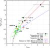 |
Fig. 13 Observed LIR/LUV ratio as a function of the UV slope β (at 2000 Å rest-frame) for our objects (black symbols), and for the local starbursts of Meurer et al. (1999; M99), revised by Takeuchi et al. (2012) in green (the corrected IRX-β curve is shown with the solid red line, and the M99 relation is shown for reference in the gray dashed line). All our values for β are the mean from the Calzetti- and the SMC-based models. For the Cosmic Eye and cB58 we plot the spectroscopically measured slopes available in the literature. The expected relation for constant SFR and age ≳100 Myr for the SMC (blue dashed-dotted) attenuation/extinction law is also plotted. High-z ULIRGs (e.g. Oteo et al. 2013) tend to populate the region above the M99 relation. Discussion in the text. |
Concerning the case of cB58, we can see that although its rest-frame UV is better fitted with a steeper SMC-like law, it lies in a region where the SMC curve and the updated M99 of Takeuchi et al. (2012) are still too close together to allow a proper distinction.
We also note that the determination of the UV slope, especially from photometry, can be quite uncertain, because systematics (e.g. the precise sampling of the UV spectrum by the filters, deviations of the spectrum from a pure power-law, etc.) and owing to random errors, making the uncertainty on individual β slopes fairly large. Figure 12 illustrates this and shows that good SED fits can yield UV slopes (here β2000 = −1.41 ± 0.2) differing quite strongly from the various published values of the UV slope of the Cosmic Eye that are usually found between −0.45 to ~010. An extensive look into the UV-spectrum publications (Smail et al. 2007; Quider et al. 2010) indicates that the slope in a range [1300 Å, 1800 Å] should be −0.45 ± 0.05, in agreement with the photometric slope between the V and I bands. Smail et al. (2007) infer a value of −1.6 ± 0.1 which is incompatible with their spectrum, and Quider et al. (2010) do not publish a value. Depending on where precisely the spectrum was sampled the slope can be vary from β ≈ −0.8 up to β ≈ 0. Our SED inferred slope centered at 1500 Å is in agreement with this bluest value, and can be accounted for as the fit’s slight deviation from the photometry at these wavelengths.
Given these uncertainties and the necessary underlying assumption on SFH, we suggest that the IRX–β plot should not be overinterpreted to distinguish different extinction/attenuation laws.
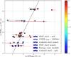 |
Fig. 14 SFRIR + SFRUV vs. SFRSED (SFRBC in the rest of the text) diagram. The straight line indicates unity. The various symbols correspond to the models shown in the key, and colors correspond to redshift according to the colorbar. For more clarity, the error bars of the models without nebular emission are in red and slight vertical shifts are imposed for all objects to better separate them. |
6.3. SFR indicators
In Fig. 14 we compare our instantaneous SFRs that our stellar models produce with observation-based total SFR, which we take as SFRIR + SFRUV, with the two terms estimated separately via the Kennicutt (1998) conversions. Overall, we have a good agreement in our sample, with only the strongly degenerated case of h7 which presents the largest spread. Our preferred model (Calzetti, declining SFH, nebular emission) reproduces SFRIR + SFRUV within 0.3 dex, and produces much more reasonable values in that regard than the same models without nebular emission that over-predict it by up to ~1 dex.
Despite our use of exponentially declining SFHs with variable timescales from τ = 0.05 to 3 Gyr we do not find any particular underestimation of SFRIR + SFRUV by the SED-derived SFRs, in contrast to the findings of Wuyts et al. (2011).
For the energy conserving models (shown as pentagons in Fig. 14), we obtain the best correspondence between SFRBC and SFRIR + SFRUV. The good agreement occurs because for most sources our fits do not yield very large values of t/τ nor extremely young ages, cases in which the assumptions made for the standard SFR calibrations may break down. The largest difference is found for A68/h7, which appears in a declining phase, with the largest value of t/τ ~ 3.6.
The relevant quantities which should be compared are the observed luminosities (IR+UV), not the SFR values derived from those using calibrations assuming a fixed SF timescale (constant SFR for this matter). Differences between SFRBC and SFRIR + SFRUV may naturally be found for models with variable SFHs, as discussed in detail in Schaerer et al. (2013).
6.4. Mass–SFR relation and specific SFR of our sample
In Fig. 15 we show the SFR as a function of the stellar mass of the seven lensed galaxies studied here, including values obtained from different models. For comparison, the sample from Daddi et al. (2007) is also plotted is as well as the mean SFR–mass relation (so-called SF main sequence) obtained for star-forming galaxies at z ~ 2. Most of the objects lie close to (i.e., within a factor of ~2) the main sequence (hereafter MS), and for most model assumptions. We can see that the classic” scenario, i.e. constant SFR, gives the smallest dispersion as seen also in Schaerer et al. (2013), but most other solutions lie still within the tight main sequence (see Rodighiero et al. 2011, defined as 4 times above the main sequence). Possible outliers are MACS0451N and nn4 (h7) whose specific SFR, sSFR = SFR/M⋆, exceeds (falls below) the median sSFR ≈ 2 Gyr-1. A68/nn4 is an extreme starburst and it is located unsurprisingly in the starburst regime (Rodighiero et al. 2011, 10 times above the main sequence). Globally, the position of our objects for varying SFHs on the M⋆– SFR diagram can be understood in terms of the median age over e-folding timescale ratio t/τ. Galaxies with a median t/τ ~ 1 − 2 in our sample lie very close to the MS, whereas A68/h7 with t/τ ~ 7 lies far below, and the ones in the starburst regime with t/τ < 1. The median solution of A68/h7 obviously must not be representative of the current star formation in that galaxy as we have seen (Fig. 4) that it also underpredicts the observed LIR which imposes an upward correction on its SFR and would bring it close to the MS.
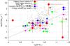 |
Fig. 15 Mass-SFR diagram, with the values obtained by the various stellar population models plus the IR-inferred SFRs (red circles: Calzetti-based exponentially declining models with nebular emission; green diamonds: same but with SMC; upwards blue triangles: the classic models assuming Calzetti, constant SFR, and tmin = 100 Myr; downwards purple triangles: IR-inferred SFRs vs. mass from SFR = const. model; black hollow diamonds: energy conserving models). Also plotted are the Daddi et al. (2007) main sequence for z ~ 2 from the GOODS field (grey continuous line), and the relation 4 times above this main sequence as shown in Rodighiero et al. (2011) (grey dot-dot-dashed line). |
However, the extreme sSFR values of these two objects are only obtained for models assuming variable, declining SF histories. Whether the true sSFR values are as high/low, could be tested with accurate, reddening corrected SFR(Hα) measurements. We note that for none of our objects do we find sSFRs as high as those obtained for z ≳ 4 LBGs in our work examining the role of nebular emission and variable SFHs for these galaxies (de Barros et al. 2012; Schaerer et al. 2013), although the same model assumptions were made.
As expected from the discussion of the individual objects, models with the SMC extinction law yield somewhat higher masses and a lower SFR, because of the preference for fits with older populations. They are, however, less favored, given the inconsistency with the observed IR luminosity for the majority of them.
The energy conserving models displace the solutions a little on the M⋆-SFR space, relative to the unconstrained ones, more so for the more extreme cases like MACS0451 and A68/h7 that become less extreme. The galaxies are still found in coherent positions with respect to their starbursting state (the t/τ ratio), with cB58 and A68/nn4 as starbursts, while A68/h7 and the Cosmic Eye (A68/C0) as post-starbursts (quiescently star-forming).
Compared to Herschel-detected galaxies from blank field studies including the deep GOODS-South data, which are restricted to SFR ≳ 100 M⊙ yr-1 and to stellar masses M⋆ ≳ 1010M⊙ (cf. Rodighiero et al. 2011), our sample includes IR-detected objects with lower SFR (up to ~1 dex) and also somewhat lower masses.
For most of the galaxies the sSFR is in the range of ~1 to 10 Gyr-1 with a median value very similar to the weighted mean specific SFR of 2.4 Gyr-1 derived for masses M⋆ ~ 108.5 − 1011M⊙ by Reddy et al. (2012b) for z ~ 1.5–2.6 galaxies combining individual IR detections and stacking results. Our sSFR values are also comparable to other determinations, e.g. for z ~ 2 − 3 LBGs by Erb et al. (2006) using SFR(Hα). As already mentioned above, the two cases of MACS0451 and A68/h7 with extreme sSFR values for some model assumptions should be taken with caution.
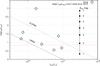 |
Fig. 16 Observed LIR/LUV luminosity ratio vs. LUV for our sample. Solid and dashed gray lines show the limits for LIRGs and ULIRGs respectively, and the pink dotted line the mean relation derived from stacking for z ~ 1.5 UV-selected galaxies by Heinis et al. (2013). On the embedded vertical axis we have the corresponding UV attenuation from Schaerer et al. (2013). The individual objects are ordered from left to right as follows: C0, HLS115, nn4, MACS0451, cB58, h7, and the Eye. |
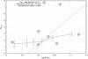 |
Fig. 17 UV extinction vs. stellar mass diagram. Plotted with the average relation and standard deviation obtained with the GOODS-Herschel sample by Buat et al. (2012) in the redshift range 0.9 < z < 2.2, after correcting it with a factor of 1.8 to account for the difference in the choice of IMFs. Also plotted is the relation from Pannella et al. (2009) for a sample of radio observed BzKs. The values shown with black diamonds are derived from the observed IR-to-UV ratio via the correspondence from Schaerer et al. (2013). |
6.5. Dust extinction as a function of stellar mass and UV luminosity
In Fig. 16 we show the observed ratio of LIR/LUV of our sample, a good measure of the UV attenuation, as a function of the UV luminosity. On the embedded vertical axis we show the corresponding UV extinction, AFUV, following the parametrization given by Schaerer et al. (2013). We note that the UV attenuation derived in this way is independent of the extinction law, because it depends on the energy redistribution between the UV and IR. Our objects span a range of ~1 dex in LIR/LUV, except for A68/nn4, which stands out because of its high IR/UV ratio of LIR/LUV ≈ 103. The corresponding UV attenuation is between AFUV ~ 1−4 (or AV ~ 0.5−1.6 for the Calzetti law). As shown in this figure, our individual IR/UV measurements are in good agreement with those derived from stacking results as a function of UV magnitude for z ~ 1.5 UV selected galaxies by Heinis et al. (2013). Our small sample and the complicated selection function does not allow us to draw any conclusions about a possible trend with LUV.
In recent years it has become clear that galaxies also show a trend of increasing extinction with stellar mass. We therefore show our results at z ~ 1.6−3 in Fig. 17, which are compared to recent results from radio and UV-stacking z ~ 2 BzK galaxies by Pannella et al. (2009), and to the median value of AFUV as a function of stellar mass derived with Herschel/PACS data from UV selected galaxies (Buat et al. 2012). As before, A68/nn4 stands out because of its very high extinction. Except for this, our individual measurements are in good agreement with these independent results also obtained for galaxies selected with different criteria. This suggests that in general star-forming galaxies show a comparable relation between extinction and stellar mass. Indeed the z ~ 1.5 − 3 galaxies plotted in this figure show a similar extinction to low-z galaxies (Martin et al. 2007; Buat et al. 2009; Whitaker et al. 2012; Domínguez et al. 2013; Zahid et al. 2013). However, given different selection criteria and the small sample size, it is difficult to understand if there is a possible redshift evolution of the dust extinction – stellar mass relation, as also discussed in Buat et al. (2012).
6.6. Dust properties
We now discuss the physical properties, temperature and mass, that we derive for the dust content of our sample from the exploitation of our IR/submm observations.
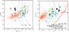 |
Fig. 18 Left: LIR vs. Tdust diagram, plotted against the larger sample of Symeonidis et al. (2013, orange dots), that of Magdis et al. (2010, green circles), and the SMG sample of (Magnelli et al. 2012a, blue diamonds). cB58 and the poorly constrained Cosmic Eye are shown by black squares surrounded by a diamond. Our sample (large hollow diamonds) has warmer Tdust compared to galaxies with same luminosity at lower redshift. Our sample has similar temperatures to the ULIRG sample of Magdis et al. (2010), indicating overall warmer temperatures at z ~ 2 or more than in the more local Universe. The SMGs that lie closest to our sample in this parameter space and appear warmer than the main SMG trend are among the most strongly lensed ones in the Magnelli et al. (2012a) sample, suggesting we have similar objects in our two surveys. The three dashed curves represent the PACS160 5σ detection limits at the redshifts mentioned below them. The smaller hollow color-coded diamonds represent the observed (lensed) luminosities of our sources, which we can see lie well above their corresponding limiting curves. Right: redshift vs. Tdust diagram. Our sample lies together the z ~ 2 ULIRGs and with many of the SMGs at same redshift. Compared to the latter in particular, our sample has similar temperatures with the SMGs that are in the ULIRG − HyLIRG regime, again indicating no strong evolution of Tdust with LIR at the considered redshifts. The rainbow colored curves represent, from left to right, the 5σ limits in Tdust per redshift for an object of respective LIR = [1,2,4,6,8,10 × 1012 L⊙]. This illustrates that for their corresponding luminosities and redshifts, our objects lie way above the minimal detectable Tdust. |
6.6.1. Dust temperature
We performed modified blackbody fits on our FIR/submm photometry (starting from restframe 40 μm and longwards), for two values of the cold end slope β = 1.5 and 2.0. As we do not have strong constraints from the submm and longwards, both values produced fits of similar quality. To allow meaningful comparison with the other studies discussed in Sect. 6.6.1, we present the temperatures for the β = 1.5 fits, as it is the value used by the mentioned publications11.
The dust temperatures obtained for our sample (Tdust in Table 3, as prescribed in the beginning of the section) cover a range between ~35 and ~55 K, typical for star-forming galaxies and starbursts. There seems to be no particular correlation between Tdust and LIR, in contrast with the trends often found in various samples (Fig. 18). Our galaxies mostly occupy the same temperature range as the star-forming ULIRGs of Magdis et al. (2010) and as the brightest (and warmest) SMGs of Magnelli et al. (2012a) at z ~ 2 − 3. Our median temperature for the sample is ≈46 K, which is very similar to the median value of 42.3 K inferred by Magdis et al. (2010). In comparison with the large sample of Symeonidis et al. (2013, this sample was carefully selected among the COSMOS and GOODS-Herschel fields in order for the properties of these galaxies to be representative of the whole IR-luminous population up to z ~ 2) our objects lie systematically on the warm side of its distribution, or above. Regarding the recent publication of Saintonge et al. (2013) and our two galaxies in common, cB58 and the Cosmic Eye, we find our estimates of Tdust to be ~5 K cooler but within reasonable range of our respective uncertainties.
This tends to show that although lensing allows us to probe much fainter galaxies at z ≥ 1.5, these galaxies are not colder than the bright ones at these redshifts. This is either indicative of a selection bias towards higher temperatures, or of a redshift – Tdust relation.
Our objects all peak around the SPIRE 250 μm band. In the redshift range of z ~ 2−3, objects of similar observed luminosity (LIR × μ ≥ 1012 L⊙) and temperatures ~15 K lower than ours would still peak within the SPIRE bands, would have higher intrinsic fluxes, and thus would be detectable. This means that only colder galaxies with lower intrinsic LIR and/or magnification would fall undetected. As an example, we can consider a galaxy at z ~ 3 with LIR × μ ≈ 1013L⊙, like the Cosmic Eye, which is easily detectable whether it peaks at 47 K (like the Eye) or at say 30 K. If it were ten times fainter, it would still be detectable in the PACS bands if at ~47 K, but would go undetected by all bands if it were at ~30 K. It seems that for the detection levels of our objects we have not reached the lowest detectable temperatures, indicating that we are not biased in that sense, but more that such IR-bright but colder objects were not to be found in the HLS fields we have explored so far. This is shown quantitatively in Fig. 18b in the rainbow colored curves where we have computed the minimal dust temperatures detectable at a given redshift for LIR values from 1012 to 1013 L⊙, corresponding to the global luminosity range of our sample. Specifically the curves represent 5σ detection limits of ~6 mJy in PACS160. In Fig. 18a we also show the same limits for luminosity and temperature at three given redshifts, representative of our sample. Our various observed luminosities lie well above their respective limits. This shows that our sample is not limited by temperature or luminosity. In addition, given the hand-picked selection of our objects and the consideration of all Herschel bands, sources detected in SPIRE but dropping out in PACS would not have gone unnoticed. The SMGs that are biased to lower temperatures and low luminosity (Magnelli et al. 2012a) occupy a strip that is only a little bit lower than our objects in the z-Tdust space, and provide a hint of the possible coldest galaxies we might detect in the global HLS sample. Magdis et al. (2012a) find a similar trend with redshift in a sample of main sequence galaxies. The same trend may not apply, however, to other galaxies such as SMGs.
6.6.2. Dust masses
In this section we present the dust masses Md for our objects that we derived from the Herschel data. One straightforward way to do this is with the help of the flux – Md calibration (Kruegel 2003) 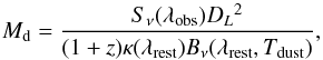 (1)where Sν(λobs) is the flux at a given observed wavelength, DL the luminosity distance, κ(λrest) the dust grain opacity per unit of dust mass, and Bν the Planck function. For the opacities we follow the calibration of Li & Draine (2001)12, given by
  (2)for 20 < λ < 700 μm, and
 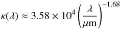 (3)for 700 < λ < 104μm. We estimate Sν from a modified blackbody fit to the Herschel and, when available, longer wavelength data with a β-slope fixed to 2, which is the form compatible with the above calibration. We present the dust masses thus obtained in Table 7. We note that this is a different fit from the one used to estimate dust temperatures, which assumes a β of 1.5. The values of Tdust and Md given here should, therefore, not be used in conjunction. This duality was needed in order to have temperatures determined in a manner consistent with those of the comparison samples taken from the literature, although these might not necessarily represent the actual temperature of any physical component. We also note that this approach is valid within the quality of our data which does not allow us to constrain well the Reyleigh-Jeans slope. We find that fits are equally good with either value of β.
Dust masses derived from MBB fits with β = 2 for our sample.
In Fig. 19 we show the derived dust masses of our lensed targets as a function of stellar mass and compare them with other recent samples, both at low and high redshift. The figure clearly shows that our measurements extend the currently available dust masses at z > 1.5 to lower values (down to Md ≈ 107M⊙), again thanks to strong lensing. Our galaxies appear to show a similar relation between dust and stellar mass to the one found for lower redshift galaxies, like the ones observed with the recent H-ATLAS/GAMA survey, or like nearby spirals or ULIRGs (cf. Santini et al. 2010; Bourne et al. 2012). They are consistent with a constant dust-to-stellar mass ratio of Md/M⋆ ≈ −2.6, the median value obtained by Smith et al. (2012) from the H-ATLAS survey. Our data indicate a continuity in M⋆−Md with the z ~ 0.5−3.5 (zmedian ≈ 2.1) submm galaxy (SMG) sample of Michałowski et al. (2010) (magenta points in Fig. 19), although Santini et al. (2010) suggest that the high-z SMGs show a higher dust/stellar mass ratio, as shown by the filled black circles.
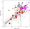 |
Fig. 19 Dust mass as a function of the stellar mass of our lensed galaxy sample (red circles) compared to other high-z (filled symbols) and local galaxy samples (open symbols). The stellar masses used here come from the energy conserving models presented in Table 6. Red triangles and blue squares (both open) show local spirals and ULIRGs; filled black circles show high-z SMGs; all data are taken from Fig. 1 of Santini et al. (2010). Filled magenta circles show the z ~ 0.5−3.5 SMG sample of Michałowski et al. (2010); yellow squares 17 z > 1 galaxies observed with Herschel in GOODS-N (Magnelli et al. 2012b); filled magenta triangles the z ~ 0.5−3 galaxies from Magdis et al. (2012a); filled black triangle the z ~ 1−2 (U)LIRG from Lo Faro et al. (2013). The green dashed line shows the location of the sequence observed by the H-ATLAS/GAMA survey at z ~ 0−0.35 (Bourne et al. 2012); the green solid line the median value of Md/M⋆ = −2.63 obtained by Smith et al. (2012) from the H-ATLAS survey after adjustment to the Salpeter IMF used here. The red solid (dotted) line shows the predictions from the chemical- and dust-evolution models of Pipino et al. (2011) for galaxies leading to the formation of ellipticals with masses of 1010 (1011) M⊙ at z = 0.; blue lines the dwarf, M101, and Milky Way models of Calura et al. (2008). The blacked shaded area (black line) shows the 68% confidence interval (median) predicted by the semi-analytical models of Lagos et al. (2012) for z ~ 1.5. The inferred dust and stellar masses of our galaxies seem to follow a simple M⋆−Md relation also extending to the SMGs. They do not show significant offsets from low redshift galaxies, and are in good agreement with the models. |
We compare our measurements with predictions of the dust content of galaxies from the chemical evolution models of Calura et al. (2008) and Pipino et al. (2011) which include dust production and destruction. These are also shown in Fig. 19. The model tracks plotted here correspond to the evolution of galaxies that become ellipticals of mass 1010 and 1011M⊙ at z = 0 as well as to the modeled evolution of the Milky Way and M101. During their star-forming phase, the models cover well the observed range of our observations and their approximate Md-M⋆ slope, and are in good agreement with the observed SFR-M⋆ values. We also show the predictions from the semi-analytical galaxy models of Lagos et al. (2012) for galaxies at z ~ 1.5. Models at other redshifts trace a very similar locus in M⋆−Md. Again, these models describe quite well the observed M⋆−Md relation of our galaxies. In short, the bulk of the data at high-z seems to follow a simple relation between stellar and dust mass, and this relation does not seem to differ significantly from the one observed at lower redshift.
We note that our galaxies show larger ratios of IR luminosity to dust mass LIR/Md, typically by a factor of ~5, than derived by Magdis et al. (2012a) from stacking for z ~ 2 galaxies with masses M⋆ ~ 1010 − 1011M⊙. Again, although systematics for the dust masses may be approximately a factor of ~2, this probably does not explain the difference. A more detailed analysis is deferred to a subsequent publication, where we also include measurements of the molecular gas mass.
6.7. Other implications
As discussed in Sects. 5.2.1 and 5.2.2, our work has led to revised stellar masses for the well-studied lensed galaxies cB58 and the Cosmic Eye found at redshift 2.7 and 3.07. Our masses are broadly in agreement with other recent studies, but are found to be a factor of 5–6 lower than earlier studies often used in the literature. The origin of the discrepancies is mostly understood (Sects. 5.2.1 and 5.2.2). For example, this implies that while Riechers et al. (2010) find that cB58 and the Cosmic Eye show high sSFRs compared to the normal population at this redshift, this is no longer the case with our results. Also, the underestimate of the stellar masses of these galaxies imply, for example, that quantities such as estimated gas fraction, gas depletion timescale, and other related quantities may need to be revised. This will be discussed in a companion paper that presents new molecular gas measurements of the lensed galaxy sample considered in this paper.
6.8. Other multi-wavelength SED models of high-z galaxies and future improvements
We now briefly discuss other recent multi-wavelength SED models and their methodology, and discuss future improvements of our method.
Although various codes allowing for multi-wavelength SED fits exist, relatively few studies of distant galaxies that analyze the combined optical, NIR, and IR SED observed with Herschel have presently been published. For example, Magdis et al. (2012b) have analyzed a small sample of z ~ 2 LBGs, but do not discuss in detail the stellar populations and properties such as the SFH and attenuation law discussed here. Buat et al. (2012) have fitted 750 UV-selected galaxies at z = 1−2 with CIGALE, a code doing energetically-consistent SED fits. They adopt a model including two separate stellar populations with an old/young component (each with a separate attenuation), and also fit a parametrized attenuation law. For ~20% of their galaxies they find indications for an attenuation law steeper than the Calzetti law. Some of their results have already been compared with ours (Sect. 6.5); others are difficult to compare. Lo Faro et al. (2013) have presented detailed fits of 31 (U)LIRG, 20 of them at z ~ 2, with the GRASIL code. This energetically consistent code takes various stellar and dust emission components into account, accounts for a variety of SFHs, and is described by a large number of parameters; (see Silva et al. 2011, for more information). From their analysis they find that all of the galaxies require the presence of an old (>1 Gyr) population, and at the same time host a moderate ongoing SF activity, i.e. a higher SFR in the past. Their model also predicts a lower SFR than expected from the IR luminosity with standard SFRIR calibrations, since a non-negligible fraction of the IR emission originates from cirrus heated by evolved stellar populations. Finally, they find that the stellar masses derived from SED fits with simple models similar to ours may be underestimated by 0.36 dex for their ULIRG sample especially for the most dusty galaxies. From their extinction, stellar mass, and LIR, only two of our objects, A68/h7 and A68/HLS115, are in a similar domain to the ULRIGs of Lo Faro et al. (2013), where their results/caveats may apply. However, given the different methodologies and different object selection, it is difficult to compare their results with ours. In particular, none of these studies compares systematically different SFHs and attenuation laws, as done here, and includes nebular emission.
We note that the CIGALE and GRASIL models applied by Buat et al. (2012) and Lo Faro et al. (2013) are more complex than ours, involving in particular several stellar populations and dust components, and more free parameters. In a first, conservative step here we have chosen much simpler SED models with a minimal number of parameters (three: age, τ, and AV), and we explore the consistency between the stellar part of the SED and the IR by verifying the energy balance between absorbed stellar and re-emitted IR radiation. Such a simple model is also motivated by the fact that similar models have often been applied for the analysis of galaxies at higher redshift, including our study of a large sample of LBGs at z ~ 3−8 (de Barros et al. 2012; Schaerer & de Barros 2010). Although our approach has lead to some interesting insight, for example on the SFHs and attenuation laws of high-z galaxies, it is not possible to demonstrate that our conclusions may not be altered if a different, more complex model was adopted. In a next step our model could include the energy balance as a constraint in the fitting procedure, in a similar fashion to CIGALE, GRASIL, or the MAGPHYS code da Cunha et al. (2008), or it could also include available emission line measurements as constraints. Obviously, an approach of this kind would reduce the uncertainties on the derived physical parameters. However, some methodological questions remain, such as whether to include observed fluxes in all the IR bands or more fundamentally the derived IR luminosity and others. These improved models will be applied in the future.
7. Summary and conclusions
We have studied in detail a small new sample of Herschel detected lensed galaxies in the redshift interval z ~ 1.6–3.2. We extended our initial five-object sample from the HLS to include two other strongly lensed star-forming galaxies that have robust Herschel detections (the Cosmic Eye, and cB58). We have extracted and compiled the photometry for our sample, covering a large wavelength range (from rest-frame UV to the FIR/submm), including observations from HST, CFHT, Spitzer, Herschel, and SCUBA2. Lensing has enabled us to extend Herschel blank field studies to lower luminosity. As seen in Fig. 3, our cases of strong lensing allow us to measure IR luminosities up to more that one order of magnitude lower than for non lensed objects.
We have performed SED-fitting of these galaxies using our modified version of the Hyperz code, modeling their stellar populations and dust emission. The large wavelength coverage enabled us to perform interesting tests in trying to distinguish various SFHs, and extinction laws, with the LIR serving as an a posteriori consistency check for the validity of the scenarios explored. The main conclusions we derive from this approach are:
-
SED models with nebular emission and variable SF historiesprovide good fits toz ~ 1.6−3 galaxies. They do not predict IR luminosities that are too high, as might have been suspected if models yielded ages that are too young. Nebular emission does not lower the age to unrealistic values, at least not if they are not preferred even before its inclusion. It also contributes to reducing the age-extinction degeneracy in some cases (see Sect. 5.1.2).
-
Although for some cases the use of the SMC extinction law produces slightly better fits in terms of
, it is not appropriate to describe our sample as it
favors old populations which underpredict the observed IR luminosity. Two cases seem
to achieve a correct prediction (nn4 and cB58), and their only common feature is that
their corresponding SMC-based models invoke young ages in contrast with the rest of
the sample (>90 Myr). -
IR luminosity in combination with emission line measurements can constrain the SFH and extinction law of SF galaxies (at least in some cases), as proposed by Schaerer et al. (2013). In particular for the Cosmic Eye, rising SFH or constant SFR can be excluded as they strongly overpredict the observed line fluxes and LIR. A declining SFH in conjunction with stronger line extinction (Calzetti 2001) is the model that reproduces the observed spectrum most accurately. The case of cB58 which also has a wide spectroscopic coverage in the literature is more mitigated in the sense that most models and both SMC and Calzetti extinction laws reproduce accurately the line measurements and observed LIR. This is probably linked to the fact that this galaxy’s population appears to be very young in age (thus not allowing for much difference to build up between the various SFHs), and has a very blue slope in the rest-frame UV (thus not allowing much distinction between the two extinction laws we explored).
-
Our normal star-forming galaxies lie close to the main sequence (Elbaz et al. 2011) even for the variable SFHs we have explored. Notable exceptions are nn4 which is a very intense starburst, MACS0451 which seems to be starbursting too but is also located in the very low stellar mass regime, and finally A68/h7 which lies far beneath the MS, but still close to it with a 1σ confidence level because of its strong degeneracy. As could be expected, the classical recipe SFH (CSFR, age prior, no nebular emission) shows less spread, and gives a flat relation in the M⋆– sSFR plane only slightly higher than the mean derive value of Reddy et al. (2012b). Lensing has enabled us to extend the M⋆-SFR diagram of IR-detected galaxies at z ~ 2 towards lower masses and SFR.
-
The comparison of the SFR indicators between the SED-inferred ones, SFR(SED), and the ones derived from the observed UV+IR luminosities via straightforward application of the Kennicutt calibrations agrees overall within 0.3 dex when considering the models with nebular emission. Calzetti-based free SFH models and no emission give systematically SFR(SED) that are too large when compared to the observationally inferred ones (~1 dex). Nevertheless, direct observables (LIR, LUV, etc.) which can be consistently derived from SED fits should be compared instead of comparing them through SFR calibrations that make specific assumptions.
-
The UV extinctions inferred from the LIR/LUV measurements is in broad agreement with the main trend derived in Buat et al. (2012), but the limited number of our sample do not allow us to state that there is a universal AUV−M⋆ relation from low to high z.
-
Furthermore, the use of the observed LIR/LUV ratio to constrain AV proves very useful in breaking the age-extinction degeneracy that many of our red-sloped galaxies suffer from, and produces population models that are coherent with the observationally derived SFR estimates. Among the declining SFHs explored, our sample shows a bimodal tendency to prefer either fast decaying bursts (τ ≤ 100 Myr) or constant star formation.
Next we sought to characterize the dust properties, namely temperature and mass, of our sample. For that we performed modified blackbody fits of the FIR/submm photometry. In our temperature analysis, we observe that our objects appear to be warmer than other star forming galaxies at low (z < 1) redshift with similar luminosity (above the median trends of the Symeonidis et al. (2013) sample, but mostly within the scatter). They actually seem to occupy the temperature ranges of more luminous objects at their corresponding redshift (Magdis et al. 2010), indicating a possible trend with z. Our sample is not temperature limited but rather luminosity limited, and although we probe luminosities up to 1 dex lower than for blank field surveys at z ~ 2 − 3, we find no evident correlation between Tdust and LIR. However, in order to robustly claim the observation of a general shift towards higher dust temperatures between the local Universe and higher redshifts, we need to conduct our analysis on the largest HLS sample possible.
The dust mass study shows our galaxies to occupy the same space as local spirals in the M⋆−Md plane and are extending samples of other studies at higher z towards lower regime (Md ≤ 107 M⊙). The stellar-dust mass relation is found in good agreement with the chemical- and dust-evolution models of Calura et al. (2008) and Pipino et al. (2011), the semi-analytical galaxy models of Lagos et al. (2012), and with observations of nearby spirals and ULIRGs (Santini et al. 2010).
This work is the first from the HLS survey to exploit the Herschel observations together with a large amount of ancillary data, covering the SED from the rest-frame UV to the IR/mm. It has shown the strength of this survey to probe the faint Universe thanks to lensing. Although the sample is very limited, our present five sources come from only 2 out of the 54 targeted clusters. The next step for our study in the immediate future is to increase our sample’s size by including sources of the other clusters.
Online material
Appendix A: Photometry tables
Restframe UV-to-FIR photometry sets for our sample (AB magnitudes up to the IRAC bands included, then in mJy) with 1σ uncertainties.
Herschel and submm/mm fluxes measured for cB58 and the Cosmic Eye after deblending (in mJy, 1σ uncertainties).
Neighboring objects within the extent of each large galaxy and to the limit of 5 mag fainter are fit simultaneously with the galaxy we want to subtract, to make sure they do not bias the fit of the larger galaxy. The neighbors are not themselves subtracted: their fluxes are remeasured from the image where the large galaxy has been subtracted. They can then be fit out and subtracted if fainter objects exist within the reach of their profile and so on.
Neighbor 4 does not have enough photometric data points in the stellar regime to constrain its redshift from that part alone. Instead, we performed global (stellar + thermal) SED fits for this object. Nevertheless, its redshift appears well-constrained as all libraries returned a best-fit redshift of z ~ 2.5. Therefore, we used z = 2.5 as the nominal redshift of Neighbor 4.
The commonly used UV spectral slope β, defined as fλ ∝ λβ, is determined between 1800 Å and 2200 Å (rest-frame) from our best-fit SEDs.
For LUV we use λ·Fλ, averaged over 1400−2200 Å, with λeff = 1800 Å.
This effect of rendering a solution older when including nebular emission seems opposite to the trend established for z ~ 3 − 6 LBGs in de Barros et al. (2012).
The IMF normalization affects stellar mass and SFR; our values need to be corrected downwards by a factor 1.7 to compare with the more realistic Chabrier IMF used by Wuyts et al. (2012).
We produce the quantity SFRIR + SFRUV by summing the SFRs derived from LUV and LIR via straightforward applications of the Kennicutt (1998) respective calibrations, presenting this way a value that accounts for both obscured and unobscured star formation.
The emission line fluxes are listed in Richard et al. (2011). The observed equivalent widths are 7.5, 60, and 20 Å for [O ii] λ3727, [O iii] λλ4959,5007, and Hβ respectively, according to Smail et al. (2007) and as measured from the NIRSPEC spectrum by Johan Richard.
Siana et al. (2009) determine β = −0.45 and ~0 from photometry and spectroscopy, respectively, and they use the mean of these two values in their analysis. We adopt this value in Fig. 13.
Tdust depends on the chosen value of β because Wien’s displacement law is modified as 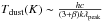 (in the case of a blackbody in the Fν formalism). For instance, the temperatures we derive for β = 2 are ≈10 − 13% lower than the ones shown in Table 3 and the figures.
Compared to Draine et al. (2003), this calibration yields dust mass a factor of 1.2 smaller.
Acknowledgments
We thank Claudio Lagos and Antonio Pipino for predictions from their models and for advice on their use. We acknowledge support for the International Team 181 from the International Space Science Institute in Berne. This work was supported by the Swiss National Science Foundation. SCUBA2 observations have been done on the James Clerk Maxwell Telescope. The James Clerk Maxwell Telescope is operated by the Joint Astronomy Centre on behalf of the Science and Technology Facilities Council of the United Kingdom, the National Research Council of Canada, and (until 31 March 2013) the Netherlands Organisation for Scientific Research. IRS acknowledges support from STFC (ST/I001573/1), a Leverhulme Fellowship, the ERC Advanced Investigator programme DUSTYGAL 321334, and a Royal Society/Wolfson Merit Award.
References
- Baker, A. J., Lutz, D., Genzel, R., Tacconi, L. J., & Lehnert, M. D. 2001, A&A, 372, L37 [NASA ADS] [CrossRef] [EDP Sciences] [Google Scholar]
- Bertin, E., & Arnouts, S. 1996, A&AS, 117, 393 [NASA ADS] [CrossRef] [EDP Sciences] [Google Scholar]
- Bolzonella, M., Miralles, J.-M., & Pelló, R. 2000, A&A, 363, 476 [NASA ADS] [Google Scholar]
- Bourne, N., Maddox, S. J., Dunne, L., et al. 2012, MNRAS, 421, 3027 [NASA ADS] [CrossRef] [Google Scholar]
- Bruzual, G., & Charlot, S. 2003, MNRAS, 344, 1000 [NASA ADS] [CrossRef] [Google Scholar]
- Buat, V., Iglesias-Páramo, J., Seibert, M., et al. 2005, ApJ, 619, L51 [NASA ADS] [CrossRef] [Google Scholar]
- Buat, V., Takeuchi, T. T., Burgarella, D., Giovannoli, E., & Murata, K. L. 2009, A&A, 507, 693 [NASA ADS] [CrossRef] [EDP Sciences] [Google Scholar]
- Buat, V., Giovannoli, E., Burgarella, D., et al. 2010, MNRAS, 409, L1 [NASA ADS] [CrossRef] [Google Scholar]
- Buat, V., Noll, S., Burgarella, D., et al. 2012, A&A, 545, A141 [NASA ADS] [CrossRef] [EDP Sciences] [Google Scholar]
- Burgarella, D., Buat, V., & Iglesias-Páramo, J. 2005a, MNRAS, 360, 1413 [NASA ADS] [CrossRef] [Google Scholar]
- Burgarella, D., Buat, V., Small, T., et al. 2005b, ApJ, 619, L63 [NASA ADS] [CrossRef] [Google Scholar]
- Burgarella, D., & PEP-HERMES-COSMOS Team 2012, Publ. Korean Astron. Soc., 27, 311 [NASA ADS] [CrossRef] [Google Scholar]
- Calura, F., Pipino, A., & Matteucci, F. 2008, A&A, 479, 669 [NASA ADS] [CrossRef] [EDP Sciences] [Google Scholar]
- Calzetti, D. 2001, PASP, 113, 1449 [NASA ADS] [CrossRef] [Google Scholar]
- Calzetti, D., Armus, L., Bohlin, R. C., et al. 2000, ApJ, 533, 682 [NASA ADS] [CrossRef] [Google Scholar]
- Casey, C. M. 2012, MNRAS, 425, 3094 [Google Scholar]
- Chapman, S. C., Blain, A. W., Smail, I., & Ivison, R. J. 2005, ApJ, 622, 772 [NASA ADS] [CrossRef] [Google Scholar]
- Chary, R., & Elbaz, D. 2001, ApJ, 556, 562 [NASA ADS] [CrossRef] [Google Scholar]
- Combes, F., Rex, M., Rawle, T. D., et al. 2012, A&A, 538, L4 [NASA ADS] [CrossRef] [EDP Sciences] [Google Scholar]
- Coppin, K. E. K., Swinbank, A. M., Neri, R., et al. 2007, ApJ, 665, 936 [NASA ADS] [CrossRef] [Google Scholar]
- da Cunha, E., Charlot, S., & Elbaz, D. 2008, MNRAS, 388, 1595 [NASA ADS] [CrossRef] [Google Scholar]
- Daddi, E., Dickinson, M., Morrison, G., et al. 2007, ApJ, 670, 156 [NASA ADS] [CrossRef] [Google Scholar]
- de Barros, S., Schaerer, D., & Stark, D. P. 2011, in SF2A-2011: Proceedings of the Annual meeting of the French Society of Astronomy and Astrophysics, eds. G. Alecian, K. Belkacem, R. Samadi, & D. Valls-Gabaud, 95 [Google Scholar]
- de Barros, S., Schaerer, D., & Stark, D. P. 2014, A&A, in press, DOI:10.1051/0004-6361/201220026 [Google Scholar]
- Domínguez, A., Siana, B., Henry, A. L., et al. 2013, ApJ, 763, 145 [NASA ADS] [CrossRef] [Google Scholar]
- Dye, S., Smail, I., Swinbank, A. M., Ebeling, H., & Edge, A. C. 2007, MNRAS, 379, 308 [NASA ADS] [CrossRef] [Google Scholar]
- Egami, E., Rex, M., Rawle, T. D., et al. 2010, A&A, 518, L12 [CrossRef] [EDP Sciences] [Google Scholar]
- Elbaz, D., Daddi, E., Le Borgne, D., et al. 2007, A&A, 468, 33 [NASA ADS] [CrossRef] [EDP Sciences] [Google Scholar]
- Elbaz, D., Dickinson, M., Hwang, H. S., et al. 2011, A&A, 533, A119 [NASA ADS] [CrossRef] [EDP Sciences] [Google Scholar]
- Ellingson, E., Yee, H. K. C., Bechtold, J., & Elston, R. 1996, ApJ, 466, L71 [NASA ADS] [CrossRef] [Google Scholar]
- Erb, D. K., Steidel, C. C., Shapley, A. E., et al. 2006, ApJ, 647, 128 [NASA ADS] [CrossRef] [Google Scholar]
- Finkelstein, S. L., Papovich, C., Giavalisco, M., et al. 2010, ApJ, 719, 1250 [Google Scholar]
- Finlator, K., Davé, R., & Oppenheimer, B. D. 2007, MNRAS, 376, 1861 [NASA ADS] [CrossRef] [Google Scholar]
- Finlator, K., Oppenheimer, B. D., & Davé, R. 2010, MNRAS, 1532 [Google Scholar]
- Finlator, K., Oppenheimer, B. D., & Davé, R. 2011, MNRAS, 410, 1703 [NASA ADS] [Google Scholar]
- Goldader, J. D., Meurer, G., Heckman, T. M., et al. 2002, ApJ, 568, 651 [NASA ADS] [CrossRef] [Google Scholar]
- Guillaume, M., Llebaria, A., Aymeric, D., Arnouts, S., & Milliard, B. 2006, in SPIE Conf. Ser. 6064, eds. E. R. Dougherty, J. T. Astola, K. O. Egiazarian, N. M. Nasrabadi, & S. A. Rizvi, 332 [Google Scholar]
- Hainline, L. J., Blain, A. W., Smail, I., et al. 2009, ApJ, 699, 1610 [NASA ADS] [CrossRef] [Google Scholar]
- Hainline, L. J., Blain, A., Smail, I., Ivison, R., & Chapman, S. 2010, BAAS, 42, 422 [NASA ADS] [Google Scholar]
- Heinis, S., Buat, V., Béthermin, M., et al. 2013, MNRAS, 429, 1113 [Google Scholar]
- Ibar, E., Sobral, D., Best, P. N., et al. 2013, MNRAS, 434, 3218 [NASA ADS] [CrossRef] [Google Scholar]
- Jones, T. A., Swinbank, A. M., Ellis, R. S., Richard, J., & Stark, D. P. 2010, MNRAS, 404, 1247 [NASA ADS] [Google Scholar]
- Kennicutt, Jr., R. C. 1998, ARA&A, 36, 189 [Google Scholar]
- Kneib, J.-P., & Natarajan, P. 2011, A&ARv, 19, 47 [Google Scholar]
- Kong, X., Charlot, S., Brinchmann, J., & Fall, S. M. 2004, MNRAS, 349, 769 [NASA ADS] [CrossRef] [Google Scholar]
- Kruegel, E. 2003, The physics of interstellar dust (Bristol: The Institute of Physics) [Google Scholar]
- Lagos, C. d. P., Bayet, E., Baugh, C. M., et al. 2012, MNRAS, 426, 2142 [NASA ADS] [CrossRef] [Google Scholar]
- Lee, K.-S., Alberts, S., Atlee, D., et al. 2012, ApJ, 758, L31 [NASA ADS] [CrossRef] [Google Scholar]
- Leitherer, C., Schaerer, D., Goldader, J. D., et al. 1999, ApJS, 123, 3 [NASA ADS] [CrossRef] [Google Scholar]
- Li, A., & Draine, B. T. 2001, ApJ, 554, 778 [Google Scholar]
- Llebaria, A., Magnelli, B., Pollo, A., et al. 2008, in Astronomical Data Analysis Software and Systems XVII, eds. R. W. Argyle, P. S. Bunclark, & J. R. Lewis, ASP Conf. Ser., 394, 589 [Google Scholar]
- Lo Faro, B., Franceschini, A., Vaccari, M., et al. 2013, ApJ, 762, 108 [NASA ADS] [CrossRef] [Google Scholar]
- Magdis, G. E., Elbaz, D., Hwang, H. S., et al. 2010, MNRAS, 409, 22 [NASA ADS] [CrossRef] [Google Scholar]
- Magdis, G. E., Daddi, E., Béthermin, M., et al. 2012a, ApJ, 760, 6 [NASA ADS] [CrossRef] [Google Scholar]
- Magdis, G. E., Daddi, E., Sargent, M., et al. 2012b, ApJ, 758, L9 [NASA ADS] [CrossRef] [Google Scholar]
- Magnelli, B., Lutz, D., Santini, P., et al. 2012a, A&A, 539, A155 [NASA ADS] [CrossRef] [EDP Sciences] [Google Scholar]
- Magnelli, B., Saintonge, A., Lutz, D., et al. 2012b, A&A, 548, A22 [NASA ADS] [CrossRef] [EDP Sciences] [Google Scholar]
- Maraston, C., Pforr, J., Renzini, A., et al. 2010, MNRAS, 407, 830 [NASA ADS] [CrossRef] [Google Scholar]
- Martin, D. C., Wyder, T. K., Schiminovich, D., et al. 2007, ApJS, 173, 342 [NASA ADS] [CrossRef] [Google Scholar]
- Meurer, G. R., Heckman, T. M., & Calzetti, D. 1999, ApJ, 521, 64 [NASA ADS] [CrossRef] [Google Scholar]
- Michałowski, M., Hjorth, J., & Watson, D. 2010, A&A, 514, A67 [NASA ADS] [CrossRef] [EDP Sciences] [Google Scholar]
- Nordon, R., Lutz, D., Saintonge, A., et al. 2013, ApJ, 762, 125 [NASA ADS] [CrossRef] [Google Scholar]
- Oesch, P. A., Labbe, I., Bouwens, R. J., et al. 2013, ApJ, 772, 136 [NASA ADS] [CrossRef] [Google Scholar]
- Oteo, I., Cepa, J., Bongiovanni, Á., et al. 2013, A&A, 554, L3 [NASA ADS] [CrossRef] [EDP Sciences] [Google Scholar]
- Pannella, M., Carilli, C. L., Daddi, E., et al. 2009, ApJ, 698, L116 [Google Scholar]
- Papovich, C., Finkelstein, S. L., Ferguson, H. C., Lotz, J. M., & Giavalisco, M. 2011, MNRAS, 412, 1123 [NASA ADS] [Google Scholar]
- Peng, C. Y., Ho, L. C., Impey, C. D., & Rix, H.-W. 2002, AJ, 124, 266 [NASA ADS] [CrossRef] [Google Scholar]
- Penner, K., Dickinson, M., Pope, A., et al. 2012, ApJ, 759, 28 [NASA ADS] [CrossRef] [Google Scholar]
- Pettini, M., Steidel, C. C., Adelberger, K. L., Dickinson, M., & Giavalisco, M. 2000, ApJ, 528, 96 [NASA ADS] [CrossRef] [Google Scholar]
- Piazzo, L., Ikhenaode, D., Natoli, P., et al. 2012, IEEE Trans. Image Process., 21, 3687 [Google Scholar]
- Pilbratt, G. L., Riedinger, J. R., Passvogel, T., et al. 2010, A&A, 518, L1 [CrossRef] [EDP Sciences] [Google Scholar]
- Pipino, A., Fan, X. L., Matteucci, F., et al. 2011, A&A, 525, A61 [NASA ADS] [CrossRef] [EDP Sciences] [Google Scholar]
- Polletta, M., Tajer, M., Maraschi, L., et al. 2007, ApJ, 663, 81 [NASA ADS] [CrossRef] [Google Scholar]
- Prevot, M. L., Lequeux, J., Prevot, L., Maurice, E., & Rocca-Volmerange, B. 1984, A&A, 132, 389 [NASA ADS] [Google Scholar]
- Quider, A. M., Shapley, A. E., Pettini, M., Steidel, C. C., & Stark, D. P. 2010, MNRAS, 402, 1467 [NASA ADS] [CrossRef] [Google Scholar]
- Rawle, T. D., Edge, A. C., Egami, E., et al. 2012, ApJ, 747, 29 [NASA ADS] [CrossRef] [Google Scholar]
- Rawle, T. D., Egami, E., Bussmann, R. S., et al. 2013, ApJ, accepted [arXiv:1310.4090] [Google Scholar]
- Reddy, N., Dickinson, M., Elbaz, D., et al. 2012a, ApJ, 744, 154 [NASA ADS] [CrossRef] [Google Scholar]
- Reddy, N. A., Pettini, M., Steidel, C. C., et al. 2012b, ApJ, 754, 25 [NASA ADS] [CrossRef] [Google Scholar]
- Renzini, A. 2009, MNRAS, 398, L58 [NASA ADS] [Google Scholar]
- Rex, M., Rawle, T. D., Egami, E., et al. 2010, A&A, 518, L13 [NASA ADS] [CrossRef] [EDP Sciences] [Google Scholar]
- Richard, J., Smith, G. P., Kneib, J.-P., et al. 2010, MNRAS, 404, 325 [NASA ADS] [Google Scholar]
- Richard, J., Jones, T., Ellis, R., et al. 2011, MNRAS, 413, 643 [NASA ADS] [CrossRef] [Google Scholar]
- Riechers, D. A., Carilli, C. L., Walter, F., & Momjian, E. 2010, ApJ, 724, L153 [NASA ADS] [CrossRef] [Google Scholar]
- Rieke, G. H., Alonso-Herrero, A., Weiner, B. J., et al. 2009, ApJ, 692, 556 [NASA ADS] [CrossRef] [Google Scholar]
- Rodighiero, G., Daddi, E., Baronchelli, I., et al. 2011, ApJ, 739, L40 [NASA ADS] [CrossRef] [Google Scholar]
- Rujopakarn, W., Rieke, G. H., Weiner, B. J., et al. 2013, ApJ, 767, 73 [NASA ADS] [CrossRef] [Google Scholar]
- Saintonge, A., Lutz, D., Genzel, R., et al. 2013, ApJ, 778, 2 [NASA ADS] [CrossRef] [Google Scholar]
- Santini, P., Maiolino, R., Magnelli, B., et al. 2010, A&A, 518, L154 [NASA ADS] [CrossRef] [EDP Sciences] [Google Scholar]
- Schaerer, D., & de Barros, S. 2009, A&A, 502, 423 [NASA ADS] [CrossRef] [EDP Sciences] [Google Scholar]
- Schaerer, D., & de Barros, S. 2010, A&A, 515, A73 [NASA ADS] [CrossRef] [EDP Sciences] [Google Scholar]
- Schaerer, D., de Barros, S., & Sklias, P. 2013, A&A, 549, A4 [NASA ADS] [CrossRef] [EDP Sciences] [Google Scholar]
- Schlegel, D. J., Finkbeiner, D. P., & Davis, M. 1998, ApJ, 500, 525 [NASA ADS] [CrossRef] [Google Scholar]
- Seitz, S., Saglia, R. P., Bender, R., et al. 1998, MNRAS, 298, 945 [NASA ADS] [CrossRef] [Google Scholar]
- Siana, B., Teplitz, H. I., Chary, R.-R., Colbert, J., & Frayer, D. T. 2008, ApJ, 689, 59 [NASA ADS] [CrossRef] [Google Scholar]
- Siana, B., Smail, I., Swinbank, A. M., et al. 2009, ApJ, 698, 1273 [NASA ADS] [CrossRef] [Google Scholar]
- Silva, L., Schurer, A., Granato, G. L., et al. 2011, MNRAS, 410, 2043 [NASA ADS] [Google Scholar]
- Smail, I., Swinbank, A. M., Richard, J., et al. 2007, ApJ, 654, L33 [NASA ADS] [CrossRef] [Google Scholar]
- Smith, D. J. B., Dunne, L., da Cunha, E., et al. 2012, MNRAS, 427, 703 [NASA ADS] [CrossRef] [Google Scholar]
- Smith, G. P., Smail, I., Kneib, J.-P., et al. 2002a, MNRAS, 330, 1 [NASA ADS] [CrossRef] [Google Scholar]
- Smith, G. P., Smail, I., Kneib, J.-P., et al. 2002b, MNRAS, 333, L16 [NASA ADS] [CrossRef] [Google Scholar]
- Symeonidis, M., Vaccari, M., Berta, S., et al. 2013, MNRAS, 431, 2317 [NASA ADS] [CrossRef] [Google Scholar]
- Takeuchi, T. T., Yuan, F.-T., Ikeyama, A., Murata, K. L., & Inoue, A. K. 2012, ApJ, 755, 144 [NASA ADS] [CrossRef] [Google Scholar]
- Teplitz, H. I., McLean, I. S., Becklin, E. E., et al. 2000, ApJ, 533, L65 [NASA ADS] [CrossRef] [PubMed] [Google Scholar]
- van der Werf, P. P., Knudsen, K. K., Labbé, I., & Franx, M. 2001, in Deep Millimeter Surveys: Implications for Galaxy Formation and Evolution, eds. J. D. Lowenthal, & D. H. Hughes, 103 [Google Scholar]
- Vibert, D., Zamojski, M., Conseil, S., et al. 2009, in SPIE Conf. Ser., 7246, 23 [Google Scholar]
- Whitaker, K. E., van Dokkum, P. G., Brammer, G., & Franx, M. 2012, ApJ, 754, L29 [NASA ADS] [CrossRef] [Google Scholar]
- Wuyts, E., Rigby, J. R., Gladders, M. D., et al. 2011, Infrared to millimeter wavelength perspective, eds. W. Wang, J. Lu, Z. Luo, et al. (San Francisco: ASP), 255 [Google Scholar]
- Wuyts, E., Rigby, J. R., Gladders, M. D., et al. 2012, ApJ, 745, 86 [NASA ADS] [CrossRef] [Google Scholar]
- Wuyts, S., Förster Schreiber, N. M., Lutz, D., et al. 2011, ApJ, 738, 106 [NASA ADS] [CrossRef] [Google Scholar]
- Yee, H. K. C., Ellingson, E., Bechtold, J., Carlberg, R. G., & Cuillandre, J.-C. 1996, AJ, 111, 1783 [NASA ADS] [CrossRef] [Google Scholar]
- Zahid, H. J., Yates, R. M., Kewley, L. J., & Kudritzki, R. P. 2013, ApJ, 763, 92 [NASA ADS] [CrossRef] [Google Scholar]
- Zamojski, M. A. 2008, Ph.D. Thesis [Google Scholar]
All Tables
Coordinates (J2000) of the five HLS sources. Redshifts of A68/C0 and A68/HLS115 come from CO observations.
Various combinations of the basic parameters that we explore in our stellar models.
Selected variable SFH models, with physical properties derived from fitting with the BC03 library.
Physical parameters derived from the energy conserving models, where AV is fixed, obtained from the observed ratio of LIR over LUV as discussed in Schaerer et al. (2013).
Restframe UV-to-FIR photometry sets for our sample (AB magnitudes up to the IRAC bands included, then in mJy) with 1σ uncertainties.
Herschel and submm/mm fluxes measured for cB58 and the Cosmic Eye after deblending (in mJy, 1σ uncertainties).
All Figures
|
Fig. 1 a) RGB rendering of A68/C0 using the F160W, F814W, and F702W HST bands. Left: images A68-C0a and A68-C0b forming a broad quasi-symmetrical arc near the cluster BCG. Upper right: third, less magnified and less distorted image, A68-C0c. Lower right: source plane reconstruction of A68-C0c after removal of the overlapping elliptical. Some residuals of the subtraction remain. b) ACS/F814W image and source plane reconstruction of A68-HLS115. Again, the neighboring elliptical has been removed in the reconstruction. c) ACS/F814W image of A68-h7 with IRAC/ch2 contours. This source consists of an interacting system of four separate components, the most extinguished of which is the southwest component. Although the exact relation of each of the components to one another is unknown, their morphology and photometry is consistent with all of them being related and forming a coherent system. d) ACS/F814W image of A68-nn4 with IRAC/ch2 contours. This source consists of a pair of interacting galaxies. We focus on the northeast component as it is the most extinguished and appears to be the most related to the IR emission. e) Left: RGB rendering of the giant arc in MACSJ0451+0006 using the F140W, F814W, and F606W HST bands. The arc is 20′′ long, and can be separated in two main components: the northern part and the southern part. The northern arc is a double image of the northern part of the source. The critical line runs through the middle of it. The southern arc is a single stretched image of the rest of the source. The two parts can be separated in Herschel up to 250 μm. The IR emission in the south appears to be dominated by an AGN, so we consider here only the northern, and starburst component, of the IR emission. Right: ACS/F606W source plane reconstruction of the arc. The morphology suggests a merger, despite ambiguious kinematics (Jones et al. 2010). |
| In the text | |
|
Fig. 2 HST/ACS image of the region around the Cosmic Eye overlaid with MIPS 24 μm emission in redscale and SPIRE 250 μm contours. Five objects, including the Cosmic Eye, blend to form a single source at 250 μm. Neighbor 4 is undetected in all of the optical bands, and faint at 24 μm, but appears in IRAC and shows up ever brighter with increasing wavelength in the infrared. Its SED indicates that it is probably an SMG an z ~ 2.5. |
| In the text | |
|
Fig. 3 IR luminosity of Herschel-detected galaxies as a function of redshift showing the position of our five lensed galaxies (open diamonds), two well-studied lensed galaxies from the literature (cB58 and the Cosmic Eye, marked as grey diamonds), and galaxies from various blank field observations, including data from the GOODS and COSMOS blank fields by Symeonidis et al. (2013) and Elbaz et al. (2011). Also plotted is the SMG sample of Magnelli et al. (2012a), and the hyLIRG detected by the HLS behind Abell 773 (Combes et al. 2012). Clearly, most of the lensed galaxies at z ~ 1.5−3 extend the blank field studies to fainter luminosities into the LIRG regime. The typical uncertainty of our LIR measurements is ± 0.1 dex or smaller. The red curve shows the minimal LIR at each redshift that can produce a flux ≥2 mJy in PACS160 (2× the confusion limit, ~3σ detection limit in GOODS-N). |
| In the text | |
|
Fig. 4 Predicted over observed ratio for LIR for all the galaxies modeled and for the different stellar population scenarios we have explored (dashed symbols stand for declining SFH models including nebular emission, solid lines neglecting this effect, dot-dashed cyan and magenta consider rising SFH scenarios including nebular emission). We can see that the SMC-based predictions underpredict LIR in almost all cases. The Calzetti-based models, although more degenerate, achieve a match with most of the objects’ observed LIRwithin the 68% confidence range. The rising SFH models predict globally at least as much or more LIR than their corresponding (in terms of extinction law) declining SFH ones (as shown in Schaerer et al. 2013), pushing in particular the Calzetti-based models to overpredict the observed quantities. The effect is similar but smaller for the SMC-based solutions, and allows a perfect match in the case of C0. We note that for MACS0451N the observed LIR of the northern part, representing ~1/3 of the total, was adopted here and the predicted LIR compared here are also derived for this same region, for coherence. This means that, depending on the model, the predicted LIR used are ~35−40% of the values listed in Tables 4 and 5. If one plotted the same for the total arc in the eventuality of a negligible AGN contribution the ratios shown would be scaled down by ~0.15 dex at most. |
| In the text | |
|
Fig. 5 Top: SED plots for A68/C0’s best stellar population fits using the two extinction laws. In the case of Calzetti, the fit including nebular emission was prefered. Bottom: global and FIR-only fits. The best fit for the full photometry uses a Seyfert galaxy template from P07 (shown in red) and an extra extinction of AV = 0.6 by the SMC law. The FIR only SED (in green) is by R09. |
| In the text | |
|
Fig. 6 Top: A68/h7 stellar population fits including nebular emission. Here the older Calzetti-based population renders the photometry longwards of 4000 Å well, but fits less the UV, and ultimately the SMC has the smallest |
| In the text | |
|
Fig. 7 Top: A68/HLS115 stellar population SEDs. The Calzetti-based model with nebular emission (green) is plotted together with the SMC-based model (red) for comparison. Although formally the best |
| In the text | |
|
Fig. 8 Top: SED plot for the A68/nn4 stellar population with non-detections shown by 1σ upper limits. For such a strongly obscured galaxy, the two extinction laws produce quite different slopes, with the Calzetti law being unable to reproduce the steep photometry at the 1σ level. Allowing for more extinction (AV ≥ 4) could not offer a better fit since this law is relatively flat, and it would have worsen the minimization in the rest-frame optical domain. The SMCibased solution, on the other hand, is steep enough. The nebular lines are relatively weak, since despite the very young age they are also absorbed, and have little effect on the solution here. Bottom: full SED fit (red), obtained with the template of IRAS 20551-4250 from the P07 library, with an additional SMC-based extinction of AV = 0.4. Given the intrinsic attenuation of the template and its characteristic 2175 Å bump, adding more extinction in order to pass beneath the 1σ-detection limits was not possible. The best fit of the FIR data (green) was obtained with the CE01 library. |
| In the text | |
|
Fig. 9 Stellar SED plot for the MACS0451 arc. Note that the F140W photometic point can only get well fitted with the help of nebular emission in the case of Calzetti’s law (green). When using the SMC law (red), this flux is matched by the combination of a Balmer break and the line emission, but the χ2 is slightly larger than the Calzetti solution. The blue curve shows that fits without nebular emission can not produce enough flux to match the F140W point. |
| In the text | |
|
Fig. 10 Top: observed and model SED for cB58. Although not a good fit, the best match to the full, global SED is found with templates from M10. We can see that the template does not match the photometry in the NUV-blue as it does not describe a population as young as is cB58’s and misses the IR peak by a factor of ~2.5. The FIR fit is obtained with a template among the brightest and warmest from CE01 that matches the IR peak very well. Bottom: SED fits to the stellar part of cB58. The red line shows the best-fit for declining SFHs, including nebular emission, and assuming the SMC extinction law. Green shows the fit neglecting nebular emission and assuming the Calzetti law (best fit among the Calzetti-based solutions). We can see that for the Calzetti law the fitted SED falls out of the 1σ uncertainty of the g-band photometry as noticed in Wuyts et al. (2012) and Siana et al. (2008). In this a case, UV slopes derived from SED fits can vary substantially depending on the extinction law used, especially around the 1300−1800 Å interval. |
| In the text | |
|
Fig. 11 Left: comparison of additional observables with model predictions for cB58 adopting the Calzetti attenuation law. Shown is the logarithmic ratio of the model prediction with respect to the observable quantity for LIR, the flux in the Hα, Hβ, [O ii] λ3727, and [O iii] λλ4959,5007 lines, as well as the Hα equivalent width. The observed values are from this paper (LIR), and from Teplitz et al. (2000). Although other emission lines have been detected in this galaxy, we do not include them here because the information they provide is basically redundant. Error bars indicate the 68% confidence interval predicted by the models; the typical observational errors, not included here, are shown with the black dotted error bars. Colors correspond to models with different SFHs (green: exponentially declining, and yellow: delayed SFHs; both for subsolar metallicity, 1/5 Z⊙. Black: SFR = const.; red: exponentially rising; both for solar metallicity). Results for the SMC law are similar and equally reproduce the observables. Right: same as left panel for the Cosmic Eye adopting the Calzetti attenuation law. Sources of the observational data are described in the text. Blue points show the predictions for models with exponentially declining SFHs and higher extinction to nebular emission (i.e. E(B − V)⋆ = 0.44 × E(B − V)neb). Red and black dashed symbols show the same for the rising and constant SFR models, respectively. |
| In the text | |
|
Fig. 12 Top: observed and model SEDs of the Cosmic Eye. The global SED is obtained with a Seyfert galaxy template from P07 but is a very poor fit, although it is the best fit among our libraries (an SMG template from M10 manages a better fit of the visible-NIR photometry, but misses the FIR data by more than one order of magnitude). The FIR data are best fitted by a R09 template, that accurately matches the photometry and 1σ limits, only slightly over-estimating the 1.2 mm detection. Bottom: comparison of the Eye’s best Calzetti fits with and without emission lines to the stellar SED. Also plotted is the very old (~1.5 Gyr) SMC-based model, which despite its large age, has favored a constant SFR and produces stronger lines than the Calzetti-based model. The difference between the three is almost imperceptible. |
| In the text | |
|
Fig. 13 Observed LIR/LUV ratio as a function of the UV slope β (at 2000 Å rest-frame) for our objects (black symbols), and for the local starbursts of Meurer et al. (1999; M99), revised by Takeuchi et al. (2012) in green (the corrected IRX-β curve is shown with the solid red line, and the M99 relation is shown for reference in the gray dashed line). All our values for β are the mean from the Calzetti- and the SMC-based models. For the Cosmic Eye and cB58 we plot the spectroscopically measured slopes available in the literature. The expected relation for constant SFR and age ≳100 Myr for the SMC (blue dashed-dotted) attenuation/extinction law is also plotted. High-z ULIRGs (e.g. Oteo et al. 2013) tend to populate the region above the M99 relation. Discussion in the text. |
| In the text | |
|
Fig. 14 SFRIR + SFRUV vs. SFRSED (SFRBC in the rest of the text) diagram. The straight line indicates unity. The various symbols correspond to the models shown in the key, and colors correspond to redshift according to the colorbar. For more clarity, the error bars of the models without nebular emission are in red and slight vertical shifts are imposed for all objects to better separate them. |
| In the text | |
|
Fig. 15 Mass-SFR diagram, with the values obtained by the various stellar population models plus the IR-inferred SFRs (red circles: Calzetti-based exponentially declining models with nebular emission; green diamonds: same but with SMC; upwards blue triangles: the classic models assuming Calzetti, constant SFR, and tmin = 100 Myr; downwards purple triangles: IR-inferred SFRs vs. mass from SFR = const. model; black hollow diamonds: energy conserving models). Also plotted are the Daddi et al. (2007) main sequence for z ~ 2 from the GOODS field (grey continuous line), and the relation 4 times above this main sequence as shown in Rodighiero et al. (2011) (grey dot-dot-dashed line). |
| In the text | |
|
Fig. 16 Observed LIR/LUV luminosity ratio vs. LUV for our sample. Solid and dashed gray lines show the limits for LIRGs and ULIRGs respectively, and the pink dotted line the mean relation derived from stacking for z ~ 1.5 UV-selected galaxies by Heinis et al. (2013). On the embedded vertical axis we have the corresponding UV attenuation from Schaerer et al. (2013). The individual objects are ordered from left to right as follows: C0, HLS115, nn4, MACS0451, cB58, h7, and the Eye. |
| In the text | |
|
Fig. 17 UV extinction vs. stellar mass diagram. Plotted with the average relation and standard deviation obtained with the GOODS-Herschel sample by Buat et al. (2012) in the redshift range 0.9 < z < 2.2, after correcting it with a factor of 1.8 to account for the difference in the choice of IMFs. Also plotted is the relation from Pannella et al. (2009) for a sample of radio observed BzKs. The values shown with black diamonds are derived from the observed IR-to-UV ratio via the correspondence from Schaerer et al. (2013). |
| In the text | |
|
Fig. 18 Left: LIR vs. Tdust diagram, plotted against the larger sample of Symeonidis et al. (2013, orange dots), that of Magdis et al. (2010, green circles), and the SMG sample of (Magnelli et al. 2012a, blue diamonds). cB58 and the poorly constrained Cosmic Eye are shown by black squares surrounded by a diamond. Our sample (large hollow diamonds) has warmer Tdust compared to galaxies with same luminosity at lower redshift. Our sample has similar temperatures to the ULIRG sample of Magdis et al. (2010), indicating overall warmer temperatures at z ~ 2 or more than in the more local Universe. The SMGs that lie closest to our sample in this parameter space and appear warmer than the main SMG trend are among the most strongly lensed ones in the Magnelli et al. (2012a) sample, suggesting we have similar objects in our two surveys. The three dashed curves represent the PACS160 5σ detection limits at the redshifts mentioned below them. The smaller hollow color-coded diamonds represent the observed (lensed) luminosities of our sources, which we can see lie well above their corresponding limiting curves. Right: redshift vs. Tdust diagram. Our sample lies together the z ~ 2 ULIRGs and with many of the SMGs at same redshift. Compared to the latter in particular, our sample has similar temperatures with the SMGs that are in the ULIRG − HyLIRG regime, again indicating no strong evolution of Tdust with LIR at the considered redshifts. The rainbow colored curves represent, from left to right, the 5σ limits in Tdust per redshift for an object of respective LIR = [1,2,4,6,8,10 × 1012 L⊙]. This illustrates that for their corresponding luminosities and redshifts, our objects lie way above the minimal detectable Tdust. |
| In the text | |
|
Fig. 19 Dust mass as a function of the stellar mass of our lensed galaxy sample (red circles) compared to other high-z (filled symbols) and local galaxy samples (open symbols). The stellar masses used here come from the energy conserving models presented in Table 6. Red triangles and blue squares (both open) show local spirals and ULIRGs; filled black circles show high-z SMGs; all data are taken from Fig. 1 of Santini et al. (2010). Filled magenta circles show the z ~ 0.5−3.5 SMG sample of Michałowski et al. (2010); yellow squares 17 z > 1 galaxies observed with Herschel in GOODS-N (Magnelli et al. 2012b); filled magenta triangles the z ~ 0.5−3 galaxies from Magdis et al. (2012a); filled black triangle the z ~ 1−2 (U)LIRG from Lo Faro et al. (2013). The green dashed line shows the location of the sequence observed by the H-ATLAS/GAMA survey at z ~ 0−0.35 (Bourne et al. 2012); the green solid line the median value of Md/M⋆ = −2.63 obtained by Smith et al. (2012) from the H-ATLAS survey after adjustment to the Salpeter IMF used here. The red solid (dotted) line shows the predictions from the chemical- and dust-evolution models of Pipino et al. (2011) for galaxies leading to the formation of ellipticals with masses of 1010 (1011) M⊙ at z = 0.; blue lines the dwarf, M101, and Milky Way models of Calura et al. (2008). The blacked shaded area (black line) shows the 68% confidence interval (median) predicted by the semi-analytical models of Lagos et al. (2012) for z ~ 1.5. The inferred dust and stellar masses of our galaxies seem to follow a simple M⋆−Md relation also extending to the SMGs. They do not show significant offsets from low redshift galaxies, and are in good agreement with the models. |
| In the text | |
Current usage metrics show cumulative count of Article Views (full-text article views including HTML views, PDF and ePub downloads, according to the available data) and Abstracts Views on Vision4Press platform.
Data correspond to usage on the plateform after 2015. The current usage metrics is available 48-96 hours after online publication and is updated daily on week days.
Initial download of the metrics may take a while.