| Issue |
A&A
Volume 561, January 2014
|
|
|---|---|---|
| Article Number | A33 | |
| Number of page(s) | 30 | |
| Section | Extragalactic astronomy | |
| DOI | https://doi.org/10.1051/0004-6361/201322338 | |
| Published online | 20 December 2013 | |
Multi-wavelength study of 14 000 star-forming galaxies from the Sloan Digital Sky Survey⋆
1
Max-Planck-Institut für Radioastronomie, Auf dem Hügel 69, 53121
Bonn, Germany
e-mail: This email address is being protected from spambots. You need JavaScript enabled to view it.
2
Main Astronomical Observatory, Ukrainian National Academy of
Sciences, Zabolotnoho
27, 03680
Kyiv,
Ukraine
3
LUTH, Observatoire de Paris, CNRS, Université Paris
Diderot, Place Jules
Janssen, 92190
Meudon,
France
4
Institut für Astrophysik, Göttingen Universität,
Friedrich-Hund-Platz 1,
37077
Göttingen,
Germany
5
Astronomy Department, King Abdulaziz University,
PO Box 80203, 21974
Jeddah, Saudi
Arabia
Received:
22
July
2013
Accepted:
16
September
2013
Abstract
We studied a large sample of ~14 000 dwarf star-forming galaxies with strong emission lines. These low-metallicity galaxies with oxygen abundances of 12 +log O/H ~7.4−8.5 are selected from the Sloan Digital Sky Survey (SDSS) and distributed in the redshift range of z ~0−0.6. We modelled spectral energy distributions (SED) of all galaxies, which were based on the SDSS spectra in the visible range of 0.38 μm−0.92 μm and included both the stellar and ionised gas emission. These SEDs were extrapolated to the UV and mid-infrared ranges to cover the wavelength range of 0.1 μm−22 μm. The SDSS spectroscopic data were supplemented by photometric data from the GALEX, SDSS, 2MASS, WISE, IRAS, and NVSS all-sky surveys. Using these data, we derived global characteristics of the galaxies, such as their element abundances, luminosities, and stellar masses. The luminosities and stellar masses range within the sample over ~5 orders of magnitude, thereby linking low-mass and low-luminosity blue compact dwarf galaxies to luminous galaxies, which are similar to high-redshift Lyman-break galaxies. It was found that the luminosity L(Hβ) of the Hβ emission line, a characteristic of the youngest stellar population with an age of a few Myr, is correlated with luminosities in other wavelength ranges. This implies that the most recent burst of star formation makes a significant contribution to the emission in the visible range and dominates in other wavelength ranges. It was also found that the contribution of the young population to the galaxy luminosity is higher for galaxies with higher L(Hβ) and higher equivalent widths EW(Hβ). We found 20 galaxies with very red WISE mid-infrared m(3.4 μm)− m(4.6 μm) colour (≥2 mag), which suggests the important contribution of the hot (with a temperature of several hundred degree) dust emission in these galaxies. Our analysis of the balance between the luminosity in the WISE bands that covered a wavelength range of 3.4 μm−22 μm and the luminosity of the emission absorbed at shorter wavelengths showed that the luminosity of the hot dust emission is increased with increasing L(Hβ) and EW(Hβ). We demonstrated that the emission emerging from young star-forming regions is the dominant dust-heating source for temperatures to several hundred degrees in the sample star-forming galaxies.
Key words: galaxies: fundamental parameters / galaxies: starburst / galaxies: ISM / galaxies: abundances
Tables 2, 3 and Figs. 10−15 are available in electronic form at http://www.aanda.org
© ESO, 2013
1. Introduction
The problems related to the formation of first galaxies at high redshifts from nearly pristine gas and the determination of their physical properties were extensively studied in recent years (e.g., Pettini et al. 2001; Stark et al. 2009; Erb et al. 2010; Schaerer & de Barros 2010). However, these studies are very difficult because of their large distances and their faintness, which leads to coarse linear resolutions and low signal-to-noise ratios. Most of the extensive high-redshift studies (e.g., Cresci et al. 2009; Förster Schreiber et al. 2009; Epinat et al. 2012) were focussed on the bright massive disc-like galaxies at z ≳ 1. Recent merger events were frequently detected in these galaxies. On the other hand, high-redshift dwarf galaxies are too faint to be detected.
The visible wavelength range of low-redshift star-forming galaxies is the most informative one for diagnostics of the ionised gas and the determination of its chemical composition. However, this part of the spectrum is shifted to the infrared range in high-redshift objects, which is strongly contaminated by the emission and absorption lines of the Earth’s atmosphere, making studies with ground-based telescopes difficult or impossible.
The situation could possibly be improved after the launch of the James Webb Space Telescope. However, there is an alternative approach to study the nearby galaxies, which are expected to have properties similar to those of distant galaxies. These galaxies may play an important role for our understanding of star-formation processes in low-metallicity environments, and they can be considered as local counterparts or analogues of high-redshift Lyman-break galaxies (LBGs). Due to their proximity, they can be studied in greater detail not resolvable in distant galaxies.
In recent years, Heckman et al. (2005) have identified nearby (z < 0.3) ultraviolet-luminous galaxies (UVLGs) selected from the Galaxy Evolution Explorer (GALEX). These compact UVLGs were eventually called Lyman-break analogues (LBAs). They resemble LBGs in several respects. In particular, their metallicities are subsolar, and their star-formation rates (SFRs) of ~4−25 M⊙ yr-1 are overlapping with those for LBGs. Gonçalves et al. (2010) studied kinematical properties of LBAs and found their striking similarities with LBGs.
Cardamone et al. (2009) selected a sample of 251 compact strongly star-forming galaxies at z ~ 0.112 − 0.36 on the basis of their green colour on the Sloan Digital Sky Survey (SDSS) composite g,r,i images (“green pea” galaxies), which again are similar to LBGs because of their low metallicity and high SFRs.
Izotov et al. (2011a) extracted a sample of 803 star-forming luminous compact galaxies (LCGs) with hydrogen Hβ luminosities L(Hβ) ≥ 3 × 1040 erg s-1 and Hβ equivalent widths EW(Hβ) ≥ 50 Å from SDSS spectroscopic data. These galaxies have properties similar to “green pea” galaxies but are distributed over a wider range of redshifts z ~ 0.02−0.63. The SFRs of LCGs are high at ~0.7−60 M⊙ yr-1 and overlap with those of LBGs.
Izotov et al. (2011a, see also Guseva et al. 2009 showed that LBGs, LCGs, luminous metal-poor star-forming galaxies (Hoyos et al. 2005), extremely metal-poor emission-line galaxies at z < 1 (Kakazu et al. 2007), and low-redshift blue compact dwarf (BCD) galaxies with strong star-formation activity obey a common luminosity-metallicity relation. Therefore, it is promising to study nearby strongly star-forming galaxies over a wide range of luminosities and metallicities to shed light on physical conditions and star-formation histories in low and high-redshift galaxies.
Number of SDSS emission-line galaxies detected in different bands.
The completion of the space GALEX survey in the UV range (Morrissey et al. 2007), the Sloan Digital Sky Survey (SDSS) in the visible range (Abazajian et al. 2009), the 2MASS survey in the near-infrared range (Skrutskie et al. 2006), the space Wide-field Infrared Survey Explorer survey (WISE, Wright et al. 2010), and the NRAO VLA Sky Survey (NVSS) in the radio continuum at 20 cm (Condon et al. 1998) opened the opportunity to study properties of large samples of star-forming galaxies over the extremely large wavelength range of ~0.15 μm−20 cm.
We used all these data bases with the aim to fit spectral energy distributions (SEDs) in ~14 000 star-forming galaxies with strong emission lines to derive global characteristics of the galaxies and the relations between them.
2. The sample
We used the whole spectroscopic data base of the SDSS DR7 (Abazajian et al. 2009), which is comprised of ~900 000 spectra of galaxies to select a sample of 14 610 spectra with strong emission lines, which do not show evidence of AGN activity. Most notable features used for this are broad lines in spectra of Sy1 galaxies and strong high-ionisation [Ne v] λ3426, He iiλ4686 emission lines in spectra of Sy2 galaxies. We select only spectra of star-forming galaxies with equivalent widths EW(Hβ) ≳ 10 Å. This selection criterion is chosen to make diagnostics of the ionised gas more reliable. In particular, dust extinction in these spectra is obtained from decrement of several hydrogen lines. Furthermore, [O iii] λ4959, 5007 emission lines were present in all spectra. They are strong in a vast majority of spectra making the determination of the chemical composition more reliable. The [O iii]λ5007/Hβ vs. [N ii]λ6583/Hα diagram for star-forming galaxies with EW(Hβ) ≳ 10 Å is shown in Fig. 1 by blue symbols. For comparison, spectra of all SDSS DR7 galaxies are shown by grey dots. The red solid line from Kauffmann et al. (2003) separates star-forming galaxies from AGNs.
There is a very small fraction of the galaxies from our sample which are located to the right from the solid line (Fig. 1) and implies some AGN activity. However, we decided to keep these galaxies in the sample. Kauffmann et al. (2003) noted that the exact separation between star-forming galaxies and AGN is subject to considerable uncertainty. Their selection of the demarcation between star-forming galaxies and AGN was subjective. It was based on the suggestion that star-forming galaxies exhibit little scatter around a single relation in the BPT diagram. However, this is not exactly the case, according to Fig. 1. There is an appreciable number of star-forming galaxies with large scatter.
A small number of selected spectra (224 spectra) represents individual H ii regions in nearby spirals but the overwhelming majority is composed of integrated spectra of galaxies from farther distances. In particular, approximately half of the galaxies have a compact structure with angular diameter not exceeding 6′′ (Table 1). We also noted that there are 452 galaxies (~3%) with two or more SDSS spectra of the same H ii region that are obtained in different epochs. We excluded spectra of H ii regions in nearby spirals and duplicate spectra. Finally, our sample included 13 934 spectra. We supplemented this data with photometric data in five SDSS bands u, g, r, i, and z.
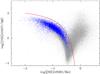 |
Fig. 1 Baldwin-Phillips-Terlevich (BPT) diagram (Baldwin et al. 1981). Selected SDSS star-forming galaxies are shown by blue filled circles. Also plotted are all emission-line galaxies from SDSS DR7 (cloud of grey dots). The red solid line from Kauffmann et al. (2003) separates star-forming galaxies from AGNs. |
The selected SDSS objects were cross-identified with sources from photometric sky surveys in other wavelength ranges, fully covering the range of equatorial coordinates of the SDSS. In spite of this we did not cross-identify sources from the Spitzer and Herschel space infrared missions since they do not fully cover the SDSS region.
In the UV range, we used GALEX far-ultraviolet (FUV; λeff = 1528 Å) and near-ultraviolet (NUV; λeff = 2271 Å) observations. We identified 86% of galaxies with GALEX sources in both the FUV and NUV bands, matching the coordinates of the objects with selected SDSS spectra within a round aperture of 6′′ in radius (Table 1).
In the near-infrared range, the SDSS sample was cross-identified with the 2MASS sources. We identified 43%, 37%, and 27% of galaxies with sources in the J (λeff = 1.22 μm), H (λeff = 1.63 μm), and Ks (λeff = 2.19 μm) bands, respectively, which indicate a lower detectability of 2MASS in comparison to GALEX (Table 1).
The coordinates of SDSS selected galaxies were used to identify sources in the WISE All-Sky Source Catalog (ASSC) within a circular aperture of 6′′ in radius. In total, 95%, 94%, 78%, and 63% of SDSS galaxies were identified with WISE sources respectively in W1 (3.4 μm), W2 (4.6 μm), W3 (12 μm), and W4 (22 μm) bands (Table 1).
Furthermore, we cross-identified the SDSS sample with sources from the IRAS far-infrared survey at 60 μm and from the NVSS survey in the continuum at 20 cm within matching radii of 6′′ and 15′′, respectively. Only a small fraction of the SDSS objects were detected in these surveys (Table 1).
Finally, the SDSS sample was cross-identified with sources from the ROSAT X-ray survey and the Planck sub-mm survey. Only a few objects within the matching radius of 20′′ were found in these surveys. Therefore, we did not use the data from the ROSAT and Planck surveys in this paper.
3. The determination of galaxy parameters
3.1. Spectroscopic data from the SDSS
The SDSS spectra were used to derive emission-line fluxes, equivalent widths, the extinction coefficient C(Hβ), the H ii region luminosity in the Hβ emission line, and chemical element abundances. First, the spectra were retrieved from the SDSS database. The observed line fluxes were obtained using the IRAF1 SPLOT routine. The line-flux errors included statistical errors in addition to errors introduced by the standard-star absolute flux calibration, which we set to 1% of the line fluxes. These errors will be later propagated into the calculation of abundance errors. The line-flux densities were corrected for two effects: (1) reddening using the extinction curve of Cardelli et al. (1989) and (2) underlying hydrogen stellar absorption that is derived simultaneously by an iterative procedure, as described in Izotov et al. (1994).
The correction for extinction was done in two steps. First, emission-line intensities with observed wavelengths were corrected for the Milky Way extinction, using values of the extinction A(V) in the V band from the NASA/IPAC Extragalactic Database (NED). Then, the internal extinction was derived from the Balmer hydrogen emission lines after correction for the Milky Way extinction. The internal extinction was applied to correct line intensities at non-redshifted wavelengths. The extinction coefficients in both cases of the Milky Way and the internal extinction are defined as C(Hβ) = 1.47E(B − V), where E(B − V) = A(V)/3.2 (Aller 1984).
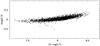 |
Fig. 2 Relation between the difference of oxygen abundances Δlog(O/H) derived by the direct and semi-empirical methods (Izotov & Thuan 2007) and the oxygen abundance obtained by the direct method. Only galaxies where [O iii] λ4363 is measured with accuracy better than 50% are shown. |
To determine element abundances, we generally followed the procedures of Izotov et al. (1994, 1997) and Thuan et al. (1995). We adopted a two-zone photoionised H ii region model: a high-ionisation zone with temperature Te(O iii), where the [O iii] lines originate, and a low-ionisation zone with temperature Te(O ii), where the [O ii] lines originate. In the H ii regions with a detected [O iii] λ4363 emission line, the temperature Te(O iii) was calculated using the direct method based on the [O iii] λ4363/(λ4959+λ5007) line ratio. In total, the [O iii] λ4363 emission line was detected in ~5700 spectra. Its flux with accuracy better than 50% was measured in ~2800 spectra.
In H ii regions where the [O iii] λ4363 emission line was not detected, we used a semi-empirical method described by Izotov & Thuan (2007) to derive Te(O iii) from the sum of line fluxes R23 = I([O ii] λ3727 + [O iii] λ4959 + [O iii] λ5007)/I(Hβ).
For Te(O ii), we used the relation between the electron temperatures Te(O iii) and Te(O ii) obtained by Izotov et al. (2006) from the H ii photoionisation models of Stasińska & Izotov (2003). Ionic and total oxygen abundances were derived using expressions for ionic abundances and ionisation correction factors (ICFs) obtained by Izotov et al. (2006).
We checked the validity of the semi-empirical method for the abundance determination comparing oxygen abundances which were derived by direct and semi-empirical methods in galaxies where both methods can be applied. We found that oxygen abundances derived by both methods agree within 0.2 dex (Fig. 2). The largest difference between direct and semi-empirical oxygen abundances was found for galaxies with 12 +log O/H ≳ 8.0. This is because Izotov & Thuan (2007) obtained the relation between Te(O iii) and R23 for galaxies with 12 +log O/H < 8.0 exhibiting “lower branch” objects on the R23 – 12 +log O/H diagram. At higher 12 +log O/H ≳ 8.0 the method described by Izotov & Thuan (2007) is less accurate.
The extinction-corrected luminosity L(Hβ) was obtained from the observed Hβ emission-line flux adopting the total extinction, which included both the Milky Way and internal galaxy extinctions, and the distance derived from the redshift. For distance determination we used the relation D = f(z,H0,ΩM,ΩΛ) from Refsdal et al. (1967), where the Hubble constant H0 = 67.3 km s-1 Mpc-1 and cosmological parameters, ΩM = 0.273 and ΩΛ = 0.682, were obtained from the Planck mission data (Planck collaboration 2013). The equivalent widths EW(Hβ) were reduced to the rest frame.
The SDSS spectra were obtained with a small aperture of 3′′ in diameter. To derive integrated characteristics of the galaxies from their spectra and to make a comparison with photometric data more accurate, we corrected spectroscopic data for the aperture using the relation 2.5r(3″)−r, where r and r(3′′) are the SDSS r-band total magnitude and the magnitude within the 3′′ spectroscopic aperture, respectively.
Throughout the paper, we used L(Hβ) in units erg s-1.
3.2. Monochromatic luminosities from the photometric data
Using photometric data from different surveys we transformed them to observed fluxes in the units of erg s-1cm-2 Å-1 in all wavelength bands for their direct comparison and the comparison to the SDSS spectroscopic data.
The fluxes  (FUV) and
(NUV) in the GALEX catalogue were expressed
in μJy. We used the effective wavelengths of 1528 Å for FUV band and 2271
Å for NUV band and the equations
(FUV) and
(NUV) in the GALEX catalogue were expressed
in μJy. We used the effective wavelengths of 1528 Å for FUV band and 2271
Å for NUV band and the equations  (1)and
 (2)respectively, to convert fluxes to the
adopted units erg s-1 cm-2 Å-1.
(2)respectively, to convert fluxes to the
adopted units erg s-1 cm-2 Å-1.
The magnitudes u, g, r,
i, and z in the SDSS bands were used to convert them
to observed fluxes: 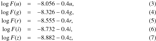 where the SDSS zeropoints were used from
Fukugita et al. (1996).
where the SDSS zeropoints were used from
Fukugita et al. (1996).
Similarly, the magnitudes in the near-infrared J, H,
and K bands were converted to the observed fluxes using the following
equations: 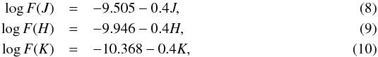 where zeropoints by Cohen et al. (2003) were used.
To convert the WISE magnitudes to fluxes, we used zeropoints by Wright et al. (2010) and the equations,
 Finally, the IRAS fluxes
(60 μm) at 60
μm in Jy, and the NVSS fluxes (20 cm) at 20 cm in mJy were converted to
the fluxes in the adopted units by using equations,
Finally, the IRAS fluxes
(60 μm) at 60
μm in Jy, and the NVSS fluxes (20 cm) at 20 cm in mJy were converted to
the fluxes in the adopted units by using equations,
 (15)and
 (16)The respective extinction-corrected
luminosities
λFλ ≡ νFν
in erg s-1 were derived from the monochromatic fluxes using the galaxy
redshift, the total extinction coefficient C(Hβ), which
included both the Milky Way and intrinsic extinctions, and the reddening law by Cardelli et al. (1989). Since the extinction at long
wavelengths is negligible, no extinction correction was applied to WISE, IRAS, and NVSS
bands.
(16)The respective extinction-corrected
luminosities
λFλ ≡ νFν
in erg s-1 were derived from the monochromatic fluxes using the galaxy
redshift, the total extinction coefficient C(Hβ), which
included both the Milky Way and intrinsic extinctions, and the reddening law by Cardelli et al. (1989). Since the extinction at long
wavelengths is negligible, no extinction correction was applied to WISE, IRAS, and NVSS
bands.
3.3. Fitting the SED from the SDSS spectra and determining the galaxy’s stellar masses
The stellar mass of a galaxy is one of its most important global characteristics. It can be derived by modelling the galaxy SED which depends on the adopted star formation history. In the case of strongly star-forming galaxies, the situation is however complicated by the presence of strong ionised gas emission, which includes the strong emission lines and gaseous continuum. Ionised gas emission must be subtracted before determining the stellar masses. In particular, neglecting the correction for gaseous continuum emission in the visible range used for the stellar mass determination would result in an overestimate of the galaxy stellar mass by ~0.4 dex (Izotov et al. 2011a) for two reasons: 1) gaseous continuum emission increases the luminosity of the galaxy; and 2) the SED of gaseous continuum emission is flatter than that of young stars, making the SED redder than expected for pure stellar emission. Consequently, the fraction of light from the red old stellar population artificially increases. To derive the correct stellar mass of the galaxy, we therefore used the method described below that considers the contribution of gaseous continuum emission, which is higher in galaxies with high equivalent widths EW(Hβ).
The method is based on fitting a series of model SEDs to the observed one and finding the best fit. This was described in Guseva et al. (2006, 2007) and Izotov et al. (2011a) and consists of the following. The fit was performed for each SDSS spectrum over the whole observed spectral range of λλ3900−9200 Å, which included the Balmer jump region (λ3646 Å) for more distant galaxies with z > 0.1 and the Paschen jump region (λ8207 Å) for galaxies with z < 0.12. As each SED is the sum of both stellar and ionised gas emission, its shape depends on the relative contribution of these two components. In galaxies with high EW(Hβ) > 100 Å, the contribution of the ionised gas emission can be large. However, the equivalent widths of the hydrogen emission lines never reach the theoretical values for pure gaseous emission, which is ~900−1000 Å for the Hβ emission line and depends slightly on the electron temperature of the ionised gas.
The objects in our SDSS sample span a lower range of EW(Hβ)s between ~10 and ~500 Å due to the contribution of stellar continuum emission. The contribution of gaseous emission relative to stellar emission can be parameterized by the equivalent width, EW(Hβ), of the Hβ emission line. Given a temperature Te(H+), the ratio of the gaseous emission to the total gaseous and stellar emission is equal to the ratio of the observed EW(Hβ) to the equivalent width of Hβ expected for pure gaseous emission. The shape of the spectrum depends also on reddening.
The extinction coefficient for the ionised gas C(Hβ) can be obtained from the observed hydrogen Balmer decrement. However, there is no direct way to derive the extinction coefficient for the stellar emission, which can be different from the ionised gas extinction coefficient in principle (Calzetti et al. 2000). For clarity, we adopted equal extinction coefficients for ionised gas and stars. Finally, the SED depends on the star-formation history of the galaxy.
We carried out a series of Monte Carlo simulations to reproduce the SED of each galaxy in our sample. To calculate the contribution of the stellar emission to the SEDs, we adopted the grid of the Padua stellar evolution models by Girardi et al. (2000) with heavy element mass fractions Z = 0.001, 0.004, and 0.008. To reproduce the SED of the stellar component with any star-formation history, we used the package PEGASE.2 (Fioc & Rocca-Volmerange 1997) to calculate a grid of instantaneous burst SEDs for a stellar mass of 1 M⊙ in a wide range of ages from 0.5 Myr to 15 Gyr. We adopted a stellar initial mass function with a Salpeter slope, an upper mass limit of 100 M⊙, and a lower mass limit of 0.1 M⊙. Then the SED with any star-formation history can be obtained by integrating the instantaneous burst SEDs over time with a specified time-varying star-formation rate.
We approximated the star-formation history in each galaxy by a recent short burst with age ty< 10 Myr, which accounts for the young stellar population, and a prior continuous star formation responsible for the older stars with age ranges starting at t2 ≡ to, where to is the age of the oldest stars in the galaxy, and ending at t1, where t2 > t1 and varies between 10 Myr and 15 Gyr. Note that zero age is now. The contribution of each stellar population to the SED was parameterized by the ratio of the masses of the old to young stellar populations, b = My/Mo, which we varied between 0.01 and 1000.
The total modelled monochromatic (gaseous and stellar) continuum flux near the Hβ emission line for a mass of 1 M⊙ was scaled to fit the monochromatic extinction- and aperture-corrected luminosity of the galaxy at the same wavelength. The scaling factor is equal to the total stellar mass M∗ in solar units. In our fitting model M∗ = My + Mo, My and Mo were respectively the masses of the young and old stellar populations in solar units. These masses were derived using M∗ and b.
The SED of the gaseous continuum was taken from Aller (1984) for λ ≤ 1 μm and from Ferland (1980) for λ> 1 μm. It included hydrogen and helium free-bound, free-free, and two-photon emission. In our models, this was always calculated with the electron temperature Te(H+) of the H+ zone and with the chemical composition derived from the H ii region spectrum. The observed emission lines that were corrected for reddening and scaled using the flux of the Hβ emission line were added to the calculated gaseous continuum. The flux ratio of the gaseous continuum to the total continuum depends on the adopted electron temperature Te(H+) in the H+ zone, since EW(Hβ) for pure gaseous emission decreases with increasing Te(H+). Given that Te(H+) is not necessarily equal to Te(O iii), we varied it in the range of (0.7−1.3) × Te(O iii). Strong emission lines in SDSS emission-line galaxies were measured with good accuracy, so the equivalent width of the Hβ emission line and the extinction coefficient for the ionised gas were accurate to 5% and 20%, respectively. Thus, we varied EW(Hβ) between 0.95 and 1.05 times its nominal value. As for the extinction coefficient C(Hβ)SED, we varied it in the range of (0.8−1.2) × C(Hβ), where C(Hβ) is the extinction coefficient derived from the observed hydrogen Balmer decrement. For each galaxy, we calculated 104 Monte Carlo models by varying ty, t1, to, b, and Te(H+) randomly in a large range and EW(Hβ) and C(Hβ)SED in a relatively smaller range because the latter quantities are more directly constrained by observations. The best modelled SED was found from χ2 minimization of the deviation between the modelled and the observed continuum in five wavelength ranges, which are free of the emission lines and residuals of the night sky lines. Depending on the galaxy redshift, the following ranges were used when possible: shortward of the Balmer jump, between the He i+H8 λ3889 and [Ne iii]+H7 λ3969 emission lines, between the Hδ and Hγ emission lines, between the He i λ4471 and [Fe iii]λ4658 emission lines, between the Hβ and He i λ5876 emission lines, between the He i λ5876 and [O i] λ6300 emission lines, and longward of the [Ar iii] λ7135 emission line but shortward of the Paschen jump.
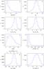 |
Fig. 3 Distribution of the SDSS emission-line galaxies a) over redshift z; b) over extinction-corrected absolute- SDSS g-magnitude Mg; c) over total stellar mass M∗; d) over mass My of the young stellar population; e) over the extinction coefficient C(Hβ); f) over the equivalent width EW(Hβ) of the Hβ emission line; g) over the extinction- and aperture-corrected Hβ luminosity L(Hβ) (lower axis) and the star-formation rate SFR (upper axis); and h) over the oxygen abundance 12 +log O/H (h). Dotted vertical lines in all panels indicate mean values of the distributions. |
4. Results
4.1. Global characteristics of the SDSS sample
In Fig. 3, we showed the distributions of some global parameters of all galaxies from the SDSS sample. The galaxies are distributed in a wide range of redshifts from 0 to 0.65 with an average value of 0.063 (Fig. 3a). Their average SDSS extinction-corrected absolute g magnitude of −19.1 mag is brighter than the brightest magnitude of −18 mag that is often used for the galaxy definition as a dwarf galaxy (Fig. 3b). The brightest galaxies in the sample have Mg as bright as ~−23 mag, which is comparable to the brightness of the high-redshift LBGs and Lyman-α emitting galaxies.
However, the aperture-corrected total stellar mass of these galaxies is low with an average value ⟨ log M∗/M⊙ ⟩ of 9.2, which is typical of dwarf galaxies (Fig. 3c). On the other hand, the mass of the young stellar populations with an age of a few Myr is high. The average ⟨ log My/M⊙ ⟩ is 7.5 implying that ~2% of the stellar mass resides in the youngest stellar complexes (Fig. 3d).
The total extinction in the direction on the SDSS sample galaxies varies in a wide range, but it is generally low with the average extinction coefficient C(Hβ) of 0.265, corresponding to an extinction AV of ~0.6 mag in the V band (Fig. 3e). On average, less than 20% of this extinction is caused by the Milky Way and the remaining extinction is the galaxy’s internal extinction.
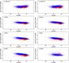 |
Fig. 4 Relations between the extinction- and aperture-corrected Hβ luminosity L(Hβ) (abscissa) and different extinction-corrected luminosity ratios (ordinates). a) The GALEX FUV-to-Hβ luminosity ratio νLν(0.15 μm)/L(Hβ) is shown. Galaxies with EW(Hβ) ≥ 50 Å and EW(Hβ) < 50 Å are shown by red and blue symbols, respectively. The galaxies with red WISE W1 − W2 ≥ 2 mag colours are shown by large filled circles. b) Same as in a) but the GALEX NUV-to-Hβ luminosity ratio νLν(0.23 μm)/L(Hβ) is shown. c) Same as in a) but the SDSS u-to-Hβ luminosity ratio νLν(0.35 μm)/L(Hβ) is shown. d) Same as in a) but the SDSS g-to-Hβ luminosity ratio νLν(0.48 μm)/L(Hβ) is shown. e) Same as in a) but the SDSS r-to-Hβ luminosity ratio νLν(0.63 μm)/L(Hβ) is shown. f) Same as in a) but the SDSS i-to-Hβ luminosity ratio νLν(0.77 μm)/L(Hβ) is shown. g) Same as in a) but the SDSS z-to-Hβ luminosity ratio νLν(0.91 μm)/L(Hβ) is shown. h) Same as in a) but the 2MASS J-to-Hβ luminosity ratio νLν(1.24 μm)/L(Hβ) is shown. i) Same as in a) but the 2MASS H-to-Hβ luminosity ratio νLν(1.66 μm)/L(Hβ) is shown. j) Same as in a) but the 2MASS K-to-Hβ luminosity ratio νLν(2.16 μm)/L(Hβ) is shown. k) Same as in a) but the WISE W1-to-Hβ luminosity ratio νLν(3.4 μm)/L(Hβ) is shown. l) Same as in a) but the WISE W2-to-Hβ luminosity ratio νLν(4.6 μm)/L(Hβ) is shown. m) Same as in a) but the WISE W3-to-Hβ luminosity ratio νLν(12 μm)/L(Hβ) is shown. n) Same as in a) but the WISE W4-to-Hβ luminosity ratio νLν(22 μm)/L(Hβ) is shown. o) Same as in a) but the IRAS 60 μm-to-Hβ luminosity ratio νLν(60 μm)/L(Hβ) is shown. p) Same as in a) but the NVSS 20 cm-to-Hβ luminosity ratio νLν(20 cm)/L(Hβ) is shown. |
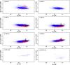 |
Fig. 4 continued. |
The average rest-frame equivalent width EW(Hβ) of the Hβ emission line of ~31 Å is modest, corresponding to the late stage of a starburst or implying an important contribution of the non-ionising stellar population (Fig. 3f). However, there are several thousand galaxies with high EW(Hβ) ≳ 50 Å and very strong emission lines. The average extinction- and aperture-corrected luminosity L(Hβ) of the Hβ emission line is high (⟨ log L(Hβ ⟩ ~ 40.6), corresponding to the ionising radiation of ~104 O7V stars (Leitherer 1990), while the entire range of L(Hβ) corresponds to the number of O7V stars that can range from a few to up to 105 (Fig. 3g). Star-formation rates SFRs are in the range 10-4−102M⊙ yr-1 with an average value of ~1 M⊙ yr-1 (upper axis in Fig. 3g).
Finally, the oxygen abundance 12 + log O/H with an averaged value of 7.95 for the entire sample is low in the SDSS star-forming galaxies (Fig. 3h). Considering that only ~2800 galaxies with the detected [O iii] λ4363 emission line had a flux was measured with an accuracy better than 50% and used a direct method, we however obtained slightly higher average oxygen abundance 12 + log O/H ~ 8.04.
Summarising the comparison of global characteristics, we concluded that the SDSS star-forming galaxies are dwarf galaxies experiencing strong and very strong bursts of star formation.
4.2. Relations between luminosities of star-forming galaxies
The relations between the star-forming galaxy luminosities in different passbands give an important information on the origin of their radiation. In particular, these relations can estimate the contribution of the young stellar population at different wavelengths. Furthermore, these relations can be used to adjust star-formation rates derived from the luminosities in different bands. As a reference luminosity, we used the extinction- and aperture-corrected luminosity L(Hβ) of the Hβ emission line, which characterises the youngest most massive stellar population. Since we selected only objects with strong emission-lines, the Hβ luminosity was derived for all spectra from the SDSS sample (Table 1).
The high detectability of the SDSS sample objects in GALEX and WISE all-sky surveys allowed us to construct reliable relations between luminosities based on large samples of star-forming galaxies.
To reduce the uncertainties due to the aperture corrections of L(Hβ) we considered relations only for compact objects with typical diameters ≲6′′. Relations between the νLν/L(Hβ) ratios and the Hβ emission-line luminosity L(Hβ) are shown in Fig. 4. To study the differences between relations in younger and older bursts we divided the sample of compact star-forming galaxies into two parts: those with the rest-frame Hβ equivalent width EW(Hβ) ≥ 50 Å (red dots) and those with EW(Hβ) < 50 Å (blue dots).
We noted that the slope of 0 in Fig. 4 corresponds to linear dependences between luminosities, which implies that radiation in these two particular wavelength ranges is produced mainly by the same young stellar population.
The common feature of the relations in Fig. 4 is that the galaxies with high EW(Hβ) ≥ 50 Å (red dots) are located below the galaxies with low EW(Hβ) < 50 Å (blue dots) because of higher Hβ luminosity. Furthermore, the slopes of relations for the galaxies with high EW(Hβ) are shallower, indicating a larger contributions of the youngest stellar population to the galaxy luminosity. Finally, negative slopes of relations in some passbands (mainly in the optical range) again indicate that the contribution of the youngest stellar population to the galaxy emission is enhanced with increasing Hβ luminosity, or equivalently, with increasing ongoing star-formation rate.
It is seen in Figs. 4a and 4b that the distributions of the νLν(0.15 μm)/L(Hβ) and νLν(0.23 μm)/L(Hβ) ratios are flat. This indicates that the emission in the Hβ line and GALEX passbands is produced by the same youngest stellar population. This is contrary to the point of view that FUV and NUV emission are indicative of an older stellar population as compared to that responsible for the ionised gas emission. Therefore, the GALEX data in strong-line emission-line galaxies can be used for the estimation of the star-formation rate of the youngest star formation episode, in addition to the Hβ emission. However, the dispersion of points in Figs. 4a and 4b is high and the SFRs estimated from the Hβ and GALEX luminosities may be different by a factor of up to ~10.
The luminosities of the SDSS galaxies with low EW(Hβ) < 50 Å in the visible (SDSS bands) range, near-infrared (2MASS bands) ranges and at 3.4 μm (WISE W1 band) are poor indicators of the most recent star formation because of the presence of negative slopes in relations as shown in Figs. 4c−4l. Contrary to that, the relations for galaxies with high EW(Hβ) ≥ 50 Å are much flatter, indicating that most of the emission in the 0.35 μm−3.4 μm range is also produced by the youngest stellar population, which is similar to that in the GALEX bands.
The luminosities at longer wavelengths, 4.6 μm−20 cm (Figs. 4m−4p), are again good tracers of the youngest stellar population independently on the EW(Hβ) value. We noted that the slope of the relations in the 12 μm and 22 μm WISE bands becomes positive and it is higher for galaxies with high EW(Hβ) (red dots in Figs. 4m−4n). Because this emission is produced by dust, we interpret the positive slopes as the consequence of increasingly hotter dust in galaxies with higher luminosities. We also noted that the dispersion of points in Fig. 4 is the lowest at 22 μm and 60 μm, allowing for an accurate SFR estimation, in addition to that derived from the Hβ luminosity.
Summarising, we concluded that the luminosities of compact galaxies with the youngest bursts and, respectively, the highest EW(Hβ) are good indicators of the most recent star-formation episode. On the other hand, only Hβ, UV, mid-infrared and radio emission are tracers of the youngest stellar population in the galaxies with low EW(Hβ).
4.3. Luminosity-metallicity and mass-metallicity relations
The luminosity-metallicity relation for emission-line galaxies from our SDSS sample is
shown in Fig. 5. We selected only 567 galaxies with
[O iii] λ4363 emission line fluxes, which were measured with an
accuracy better than 25%. Oxygen abundances in these galaxies were derived by the direct
method. Furthermore, we selected only compact galaxies with angular diameters ≲6′′.
Therefore, the oxygen abundance in these galaxies is a characteristic of the entire
galaxy, not of its individual H ii regions. The maximum likelihood regression,
 (17)is shown by a solid line. Galaxies with high
SFR(Hα) ≥ 10
M⊙ yr-1 are encircled. They are among the most
luminous objects in the sample. There is no evident offset from the linear regression of
the encircled galaxies.
(17)is shown by a solid line. Galaxies with high
SFR(Hα) ≥ 10
M⊙ yr-1 are encircled. They are among the most
luminous objects in the sample. There is no evident offset from the linear regression of
the encircled galaxies.
The relation in Eq. (17) is flatter than that obtained by Guseva et al. (2009) and Izotov et al. (2011a). However, we noted that the SDSS sample is lacking very metal-poor galaxies. On the other hand, authors of mentioned papers considered not only SDSS galaxies but also galaxies from other samples consisting of the most metal-deficient galaxies or of the galaxies where the oxygen abundances were derived by the strong-line method. Our sample, which is a variation to this, is more uniform and includes only objects where the oxygen abundance was derived using a direct Te method.
Our luminosity-metallicity relation is also much flatter compared to that obtained by Tremonti et al. (2004) for a sample of ~53 000 star-forming galaxies selected from the SDSS. We noted that selection criteria are different for these two SDSS samples. Tremonti et al. (2004) selected mainly galaxies with low-excitation H ii regions, where the [O iii] λ4363 emission is not detected and the strong lines were used for the oxygen abundance determination. Most of the galaxies in the Tremonti et al. (2004) sample have 12 + log O/H >8.6.
In Fig. 6a, we showed the mass-metallicity relation
for our sample galaxies. We selected the same galaxies as in the luminosity-metallicity
relation (Fig. 5). It is seen that galaxies with
lower mass have systematically lower oxygen abundances. These lower-mass galaxies are
primarily those with high EW(Hβ). The data can be fitted
by a linear relation, as shown in Fig. 6a by the
solid line,  (18)The relation in Eq. (18) is steeper and is better defined compared
to the relation by Izotov et al. (2011a) for LCGs,
which are the most massive galaxies of the SDSS sample of compact star-forming galaxies.
This is because the galaxies from our sample have a larger range of stellar masses as
compared to LCGs and include faint dwarf emission-line galaxies.
(18)The relation in Eq. (18) is steeper and is better defined compared
to the relation by Izotov et al. (2011a) for LCGs,
which are the most massive galaxies of the SDSS sample of compact star-forming galaxies.
This is because the galaxies from our sample have a larger range of stellar masses as
compared to LCGs and include faint dwarf emission-line galaxies.
On the other hand, the mass-metallicity relation in Fig 6a (solid line) is much flatter and is shifted to lower metallicities compared to that obtained by Tremonti et al. (2004) (dashed line). As for the luminosity-metallicity relation, this difference is likely caused by different selection criteria and different methods used for the oxygen abundance determination. Furthermore, no constraints on the morphology were given by Tremonti et al. (2004), while we used only compact objects and considered aperture corrections. Therefore, aperture effects in the mass determination played a minor role for our sample of SDSS galaxies.
It was argued in some recent papers (e.g. Manucci et al. 2010; Lara-López et al. 2010; Hunt et al. 2012; Andrews & Martini 2013) that star-forming galaxies with higher SFR are systematically more metal-poor on the mass-metallicity diagrams. We checked whether this tendency is present for galaxies from our sample. For this, we encircled galaxies with high SFRs ≥ 10 M⊙ yr-1. We concluded from Fig. 6a that the galaxies with high SFRs and the best-derived oxygen abundances are not systematically more metal-poor, which is contrary to conclusions in papers mentioned above.
Figure 6b shows the dependence of the oxygen abundance 12 + log O/H on the mass of the young stellar population formed in the most recent burst of star formation; the ages of the papulation are between 0 and 10 Myr. To our knowledge, this relation has never been discussed before. As for the mass-metallicity relation, the mass of young stellar population is gradually decreasing with decreasing metallicity. However, the slope of the relation in Fig. 6b is slightly flatter than that for the mass-metallicity relation, which addresses the entire stellar mass in Fig. 6a.
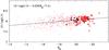 |
Fig. 5 Luminosity-metallicity relation. Symbols are the same as in Fig. 4. Linear likelihood regression is shown by solid line. Only 567 galaxies where the errors in [O iii] 4363 emission-line flux do not exceed 25% are also shown. The galaxies with red WISE colours W1 − W2 ≥ 2 mag are indicated by large black filled circles and the galaxies with SFR(Hα) ≥ 10 M⊙ yr-1 are encircled. |
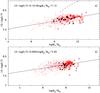 |
Fig. 6 a) Mass-metallicity relation. Symbols are the same as in Fig. 4. The linear likelihood regression is shown by solid line. The sample of galaxies is the same as in Fig. 5. The galaxies with red WISE colours W1 − W2 ≥ 2 mag are indicated by large black filled circles and the galaxies with SFR(Hα) ≥ 10 M⊙ yr-1 are encircled. For comparison, the mass-metallicity relation for 53 000 SDSS star-forming galaxies (Tremonti et al. 2004) is shown by a dashed line. b) Relation between the mass of the young stellar population and the oxygen abundance. The linear likelihood regression is shown by solid line. The galaxies with red WISE colours W1 − W2 ≥ 2 mag are resembled by large black filled circles and the galaxies with SFR(Hα) ≥ 10 M⊙ yr-1 are encircled. |
4.4. Colour–colour diagrams and galaxies with hot dust emission
The completion of the WISE All-Sky Source Catalogue (ASSC) in 2011 offered an opportunity in the search for star-forming galaxies with hot dust emission. First results in this direction were demonstrated by Griffith et al. (2011) and Izotov et al. (2011b), who found three and four galaxies respectively with very red 3.4 μm−4.6 μm colours, indicating the rapid increase of the dust emission in the 3.4−4.6 μm range, the signature of hot dust. These findings were based on the data from the Preliminary Release Source Catalogue (PRSC), which covered only half of the sky.
Several galaxy components can contribute to the emission in the 3.4−4.6 μm range: stars, ionised gas, polycyclic aromatic hydrocarbon (PAH) emission, and hot dust. However, the PAH emission is weak in a low-metallicity environment (Engelbracht et al. 2008; Hunt et al. 2010). Using results from the SED modelling of Sect. 4.5, we found that stellar and interstellar ionised gas emission are characterised by W1 − W2 colours of ~0 and ~0.7 mag, respectively (see also Table 1 in Wright et al. 2010). This indicates a steeper decline of stellar emission. Therefore, a colour excess above W1 − W2 ~ 0.7 mag could be an indication of hot dust with a temperature of several hundred Kelvin. However, the W1 − W2 colour alone is not sufficient for a precise determination of the dust temperature. The SED is needed in a wide wavelength range to fit and subtract stellar and gaseous emission.
In Fig. 7, we showed the W1 − W2 vs W2 − W3 colour–colour diagram for ~10 000 galaxies from the SDSS sample that excludes galaxies, which were not detected in each of the W1, W2, and W3 bands. The sample in Fig. 7a is split into two subsamples of objects with EW(Hβ) ≥ 50 Å (magenta dots) and EW(Hβ) < 50 Å (cyan dots). Twenty galaxies with W1 − W2 ≥ 2 mag are shown by large black filled circles. Four of these galaxies were discovered by Izotov et al. (2011b). With the ASSC, we added sixteen more galaxies with very red W1 − W2 colour. Similarly, we split the sample into two subsamples of objects in Fig. 7b with the Hβ luminosity L(Hβ) ≥ 3 × 1040 erg s-1 (orange dots) that corresponds to a star-formation rate SFR(Hα) ≥ 0.7 M⊙ yr-1 (according to prescriptions of Kennicutt 1998) and L(Hβ) < 3 × 1040 erg s-1 (green dots). Finally, we split the sample into two subsamples of objects with EW(Hβ) ≥ 50 Å and L(Hβ) ≥ 3 × 1040 erg s-1 (red dots) and EW(Hβ) < 50 Å and L(Hβ) < 3 × 1040 erg s-1 (blue dots) in Fig. 7c. The galaxies shown in red correspond to the LCGs discussed by Izotov et al. (2011a). For comparison, the cloud of grey dots is the sample of SDSS QSOs (Schneider et al. 2010). It is seen that QSOs are well distinct from star-forming galaxies.
Most of the galaxies (~90%) from our sample have blue W1 − W2 colours of ≲0.5 mag, which are consistent with the stellar and ionised gas emission, when only as a main source of radiation. Similarly to Izotov et al. (2011b), we found that galaxies with red W1 − W2 colours greater than 1 mag are mainly luminous galaxies with high-excitation H ii regions. This is most clearly seen in Fig. 7c where the red points diverge most notably from the blue ones. This finding suggests that the emission seen in the WISE bands and produced by hot dust is caused by the radiation from young star-forming regions.
In Fig. 8, we show the GALEX m(FUV)−SDSS r vs. WISE W1 − W4 colour-colour diagram. There is a clear separation between the faint galaxies with low-excitation H ii regions (blue dots) from the luminous galaxies with high-excitation H ii regions, which again implies that star-forming regions are the main source of hot dust heating. The galaxies with the reddest W1 − W2 colours (large black filled circles) are also among the galaxies with the reddest W1 − W4 colours.
Figure 8 also implies that SDSS star-forming galaxies are relatively transparent systems and only a small fraction of UV radiation is transformed into the emission in the mid-infrared range as seen by WISE. The same conclusion comes from the distribution of extinction coefficient C(Hβ) (Fig. 3e) and the comparison of the GALEX FUV and NUV luminosities (Figs. 4a and 4b) with WISE luminosities (Figs. 4k−4n). It is seen that luminosities in WISE bands are only ~10%−30% of those in GALEX bands.
In Fig. 9, we showed the relation between WISE W1 − W2 colour and oxygen abundance 12 + log O/H. The lowest-metallicity galaxies with 12 + log O/H < 7.6 were found mainly among the SDSS galaxies with low Hβ luminosity and blue W1 − W2 colours (blue symbols); the latter are consistent with stellar and ionised gas emission. The contribution of hot dust in these galaxies is small. Only few galaxies with L(Hβ) ≥ 3 × 1040 erg s-1 have the oxygen abundances of ~7.5−7.6. Most of the luminous SDSS galaxies have oxygen abundances above 8.0 (red symbols). There is no clear dependence of the W1 − W2 colour on the oxygen abundance, despite the already mentioned fact that lowest-metallicity galaxies are mainly blue.
However, there is one exception. This is the BCD SBS 0335–052E with 12 + log O/H = 7.3 (Fig. 9). First, Thuan et al. (1999) with ISO spectroscopic observations and later Houck et al. (2004) with Spitzer spectroscopic observations showed that mid-infrared emission in this galaxy is dominated by warm dust. The WISE photometric observations (Griffith et al. 2011) confirmed these findings. All galaxies with the red W1 − W2 colour found in this paper (large black filled circles) are high-metallicity analogues of the three lower-metallicity galaxies (asterisks) discussed by Griffith et al. (2011). Similar to other galaxies shown in Fig. 9, there is no evident dependence of the W1 − W2 colour with oxygen abundance among the galaxies with the reddest WISE colours.
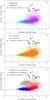 |
Fig. 7 a)m(3.4 μm)− m(4.6 μm) vs. m(4.6 μm)−m(12 μm) colour–colour diagram for a sample of emission-line galaxies detected in the three WISE bands 3.4 μm (W1), 4.6 μm (W2), and 12 μm (W3). Galaxies with Hβ equivalent width EW(Hβ) ≥ 50 Å are shown by magenta filled circles while galaxies with EW(Hβ) < 50 Å are shown by cyan open circles. Twenty newly identified galaxies with m(3.4 μm)−m(4.6 μm) ≥ 2 mag are shown by large black filled circles. b) Same as in a) but galaxies with Hβ luminosity L(Hβ) ≥ 3 × 1040 erg s-1 are shown by orange filled circles while galaxies with L(Hβ) < 3 × 1040 erg s-1 are shown by green open circles. c) Same as in a) but galaxies with Hβ luminosity L(Hβ) ≥ 3 × 1040 erg s-1 and with Hβ equivalent width EW(Hβ) ≥ 50 Å are shown by red filled circles while galaxies with L(Hβ) < 3 × 1040 erg s-1 and with EW(Hβ) < 50 Å are shown by blue open circles. For comparison, gray dots in (c) show the location of QSOs selected in the SDSS. |
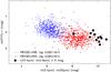 |
Fig. 8 m(3.4 μm)−m(22 μm) vs. m(FUV)−r colour–colour diagram for a sample of emission-line galaxies detected in the WISE 3.4 μm (W1) and 22 μm (W4) bands and in the GALEX FUV band. Galaxies with Hβ equivalent width EW(Hβ) ≥ 50 Å and with L(Hβ) ≥ 3 × 1040 erg s-1 are shown by red filled circles, while galaxies with EW(Hβ) < 50 Å and with L(Hβ) < 3 × 1040 erg s-1 are depicted by blue open circles. Galaxies with m(3.4 μm)−m(4.6 μm)≥ 2 mag are shown by large black filled circles. |
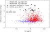 |
Fig. 9 m(3.4 μm)−m(4.6 μm) vs. 12 +log O/H diagram for a sample of emission-line galaxies detected in WISE 3.4 μm (W1) and 4.6 μm (W2) bands. Galaxies with Hβ equivalent width EW(Hβ) ≥ 50 Å and with L(Hβ) ≥ 3 × 1040 erg s-1 are shown by red filled circles while galaxies with EW(Hβ) < 50 Å and with L(Hβ) < 3 × 1040 erg s-1 are shown by blue open circles. Galaxies with m(3.4 μm)−m(4.6 μm)≥ 2 mag from this paper are shown by large black filled circles and from Griffith et al. (2011) by asterisks. Only the galaxies where the errors in [O iii] λ4363 emission-line flux do not exceed 50% are shown. |
4.5. Morphology and SEDs of the galaxies with hot dust emission
The galaxies with very red colours W1 − W2 ≥ 2 mag are rare. Griffith et al. (2011) found three galaxies that are not present in our sample, because no SDSS spectra are available for them. We found only twenty more galaxies like these out of ~14 000 galaxies from our SDSS sample with the available WISE data. The observed characteristics of these galaxies are shown in Table 2; the derived parameters are present in Table 3. For the sake of comparison, we also show the parameters of all 64 galaxies with 2 mag >W1 − W2 ≥ 1.5 mag and a representative sample of 10 galaxies with blue colours W1 − W2 < 0.5 mag in Tables 2 and 3. In general, galaxies with the reddest W1 − W2 colours are apparently faint but intrinsically bright with L(Hβ), which corresponds to SFR ~ 3−47 M⊙ yr-1 and is similar to that in high-redshift LBGs. Despite the high absolute brightness, their stellar masses of 108−109M⊙ are typical of dwarf galaxies.
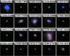
The SDSS composite g,r,i images of galaxies with W1 − W2 ≥ 2 mag, 2 mag > W1 − W2 ≥ 1.5 mag, and W1 − W2 < 0.5 mag are shown in Figs. 10−12, respectively. All galaxies with the reddest W1 − W2 colours are compact (Fig. 10) with angular diameters ≤1′′−2′′, corresponding to linear diameters ~3−6 kpc at the redshifts of 0.15−0.3. They can be classified as “green pea” (Cardamone et al. 2009) and/or LCGs (Izotov et al. 2011a). For comparison, the sample of galaxies with bluer colours (Figs. 11 and 12) include not only compact but also extended objects and objects with multiple knots.
Modelled and aperture-corrected observed SEDs for twenty galaxies with the reddest W1 − W2 are shown in Fig. 13. We produced modelled SEDs (blue lines) based on the observed SDSS spectra (black lines), which were extrapolated to the UV and IR ranges. They include the modelled stellar SEDs (green lines) and modelled ionised gas SEDs (magenta lines). For comparison, we show photometric data from GALEX, SDSS, 2MASS and WISE by red symbols and red lines. These data were transformed to units erg s-1 cm-2 Å-1 using equations in Sect. 3.2. However, we note that photometric data are not used for modelling of the SEDs. Nevertheless, photometric data agree with the modelled SEDs, such as in the GALEX FUV and NUV ranges. This is because all objects with the reddest W1 − W2 colours are compact with angular diameters that are comparable to that of the SDSS spectroscopic aperture. Therefore, the uncertainties introduced by aperture corrections are small.
Some photometric data in the visual range (SDSS g, r, i and z) show an excess above the continuum, which can exceed ~1.5 mag in some cases. This excess is due to a significant contribution of strong emission lines. We also noted that the contribution of the ionised gas emission is increased with increasing wavelength, and in some galaxies with high EW(Hβ) (e.g. J1327+6151 in Fig. 13), it is dominant longward of the K band. Therefore, it is important to consider this emission as to not misinterpret it as the emission of cool stars and hence not to overestimate the galaxy stellar mass (see, e.g. Izotov et al. 2011a). On the other hand, strong excess emission is seen in the WISE bands (red filled circles connected by solid lines) suggesting a dominating contribution of dust emission in this wavelength range. While the emission at 3.4 μm is still close to the value predicted for the combined stellar and ionised gas emission, it is higher by 1−2 orders of magnitude at 4.6 μm and continues to rise longward.
The SEDs of all galaxies with 2 mag >W1 − W2 ≥ 1.5 mag and of ten representative galaxies with W1 − W2 < 0.5 mag are shown in Figs. 14 and 15, respectively. The continuum in the mid-infrared range for objects in Fig. 14 does not rise so steeply, as in the case of objects in Fig. 13. As for galaxies with blue W1 − W2 colours (Fig. 15), the emission decreases in the wavelength range 3.4 μm−4.6 μm and agrees with the modelled combined stellar and ionised gas emission but increases at longer wavelengths, suggesting that the contribution of the hot dust is not as large as in the case of the galaxies with redder W1 − W2 colours. As noted, in the case of extended galaxies (e.g., J0849+1114 and J0949+1750 in Fig. 14), photometric data strongly deviate from the spectroscopic fits.
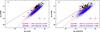 |
Fig. 16 a) Dependence of the luminosity L(WISE) integrated over all WISE bands in the wavelength range 3.4 μm−22 μm on the total extinction-corrected luminosity L(total) in the wavelength range 0.1 μm−22 μm. Galaxies with EW(Hβ) ≥ 50 Å and EW(Hβ) < 50 Å are shown by red and blue symbols, respectively. Galaxies with m(3.4 μm)−m(4.6 μm) ≥1.5 mag are shown by large black filled circles. Solid line is the line of equal values; dotted and dashed lines are maximum likelihood fits to the sample galaxies with EW(Hβ) ≥ 50 Å and EW(Hβ) < 50 Å, respectively. Error bars are average dispersions of the data around the fits. b) Dependence of the luminosity L(WISE) on the luminosity L(absorbed) of the absorbed emission in the wavelength range 0.1 μm−3 μm. The meaning of lines and symbols is the same as in a). |
4.6. Energy balance for the SDSS dwarf emission-line galaxies
The large wavelength coverage from 0.1 μm to 22 μm of our galaxy fits and the large sample allowed us to statistically study the energy balance for all SDSS spectra of emission-line galaxies. Some part of the galaxy emission is absorbed by dust at short wavelengths. It heats dust and is re-emitted in the infrared range. In particular, it is interesting to study what fraction of emission in the infrared is due to the hot dust.
We used the modelled SEDs (some examples are present in Figs. 13−15) and WISE photometric data
to calculate the total extinction-corrected luminosity of the galaxy
L(total) in the wavelength range 0.1 μm−22
μm:  (19)where λ and
λ(1 + z) are rest-frame and observed wavelengths,
Lλ is the rest-frame monochromatic
luminosity non-corrected for extinction,
Aλ(1 + z)(MW) is the
Milky Way extinction at the observed wavelength, and
Aλ(int) is the internal galaxy extinction
at the rest-frame wavelength. We also calculated the luminosity of the absorbed emission
L(absorbed) in the wavelength range 0.1 μm−3
μm by subtracting the galaxy luminosity corrected for the Milky Way
extinction (but not for the internal extinction) from the luminosity corrected for both
the Milky Way and galaxy internal extinction:
(19)where λ and
λ(1 + z) are rest-frame and observed wavelengths,
Lλ is the rest-frame monochromatic
luminosity non-corrected for extinction,
Aλ(1 + z)(MW) is the
Milky Way extinction at the observed wavelength, and
Aλ(int) is the internal galaxy extinction
at the rest-frame wavelength. We also calculated the luminosity of the absorbed emission
L(absorbed) in the wavelength range 0.1 μm−3
μm by subtracting the galaxy luminosity corrected for the Milky Way
extinction (but not for the internal extinction) from the luminosity corrected for both
the Milky Way and galaxy internal extinction: 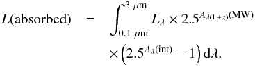 (20)Finally, we calculated the galaxy luminosity
L(WISE) in the wavelength range 3.4 μm−22
μm by using WISE photometric data. To reduce the uncertainties of
aperture corrections, however, we restricted ourselves to the consideration of compact
galaxies, which only comprises roughly half of the entire SDSS sample.
(20)Finally, we calculated the galaxy luminosity
L(WISE) in the wavelength range 3.4 μm−22
μm by using WISE photometric data. To reduce the uncertainties of
aperture corrections, however, we restricted ourselves to the consideration of compact
galaxies, which only comprises roughly half of the entire SDSS sample.
In Fig. 16a, we showed the dependence of L(WISE) on the total galaxy luminosity L(total). The total luminosity was varied in a wide range from ~107L⊙ to ~1012L⊙. The solid line in the Figure is a line of equal luminosities. It is seen that the fraction of the luminosity in the WISE bands at the low-luminosity end is ≲1% of the total luminosity (red and blue dots), but it is gradually increased to ~10% at the high-luminosity end. This fraction is also higher for galaxies with high EW(Hβ) ≥ 50 Å, which contain the dominating part of the hot dust emission. The largest fraction of the WISE luminosity is emitted in galaxies with red W1 − W2 colours. For galaxies with W1 − W2 ≥ 1.5 mag (large black filled circles), it may be as high as ~50% of L(total).
The dependence of the luminosity L(WISE) in the WISE bands on the luminosity L(absorbed) is shown in Fig. 16b. The solid line is the line of equal luminosities. The fraction of the radiation emitted by dust in the WISE bands is ~10% in galaxies with low EW(Hβ) < 50 Å (blue dots), and it is higher by a factor of ~3 in galaxies with high EW(Hβ) ≥ 50 Å (red dots), which again indicates the dominant role of young starbursts in heating the dust to high temperatures. As for galaxies with red W1 − W2 colours (≥1.5 mag), L(WISE) is comparable to L(absorbed) (large black filled circles). We concluded that the contribution of hot dust in the infrared emission is high and possibly is dominated in galaxies with the red W1 − W2 colours.
We have only scarce data from the IRAS 60 μm band because of the low IRAS sensitivity. For compact galaxies, which were detected by both IRAS and WISE, we show the dependence of the luminosity ratio L(WISE)/νLν(60 μm) vs W1 − W2 colour in Fig. 17. Because L(WISE) and νLν(60 μm) are tracers of hot (several hundred K) and cooler (several ten K) dust, respectively, the luminosity ratio tells us what the fraction of the infrared emission from the hot dust is. This is seen in Fig. 17 when L(WISE)/νLν(60 μm) is higher in galaxies with redder W1 − W2 colours and approaches ~1 in the reddest galaxies. It is also higher in galaxies with high L(Hβ) (red and black symbols), which again implies that dust is heated to high temperatures by young star-forming regions with an age of a few Myr.
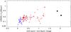 |
Fig. 17 Ratio L(WISE)/νLν(60 μm) vs. WISE W1 − W2 colour for the compact galaxies from the SDSS sample. Galaxies with L(Hβ) ≥ 3 × 1040 erg s-1 and L(Hβ) < 3 × 1040 erg s-1 are shown by red and blue dots, respectively. Galaxies with W1 − W2 ≥ 1.5 mag are shown by large black filled circles. |
5. Summary
We studied a large sample of ~14 000 SDSS emission-line star-forming galaxies. These data are supplemented by data from the GALEX survey in the UV range, the 2MASS survey in the near-infrared range, the WISE survey in the mid-infrared range, the IRAS survey in the far-infrared range, and the NVSS survey in the radio continuum at 20 cm. Using the SDSS spectra in the visible range, we fitted the SEDs by considering both the stellar and the ionised gas emission. These fits were extrapolated to the UV and mid-infrared ranges.
We also searched for star-forming SDSS galaxies with an aim to find galaxies with hot dust emission at wavelengths of λ3.4−4.6 μm (WISE W1 and W2 bands).
Our main results are as follows.
-
1.
We found that ~12 500 and ~13 500 galaxies out of the total sample of SDSS galaxies were detected by GALEX and WISE, respectively. Roughly half of the selected SDSS galaxies are compact systems. This allowed us to compare the global galaxy characteristics derived from the spectroscopic and photometric data.
-
2.
The luminosities obtained from the photometric observations in a wide wavelength range from the UV to the radio range are correlated with the luminosity L(Hβ) of the Hβ emission line, which implies that young star-forming regions strongly contribute to the emission of the galaxies. This contribution becomes more notable with a rising L(Hβ) and the equivalent width EW(Hβ) of the Hβ emission line. The luminosities of star-forming galaxies vary over a large range. At highest luminosities of ~1012L⊙, they approach the luminosities of high-redshift LBGs, implying that these galaxies can be considered as the local counterparts of distant forming galaxies in the early Universe. On the other hand, their stellar masses are low but similar to that of LBGs with an average value of ~109M⊙. This suggests that selected SDSS galaxies are dwarf systems with luminosities elevated by the strong ongoing star formation with SFRs up to ~100 M⊙ yr-1.
-
3.
A major fraction of galaxies has WISE W1 − W2 colours of ~0.0−0.4 mag, which are consistent with the colour for the emission from stars and the ionised interstellar medium. The contribution of hot dust with temperatures of several hundred degrees to the mid-infrared emission is small in these galaxies. On the other hand, we found 20 galaxies with redder colours, W1 − W2 ≥ 2 mag. Most of these galaxies are LCGs with star-formation rates SFR(Hα) > 0.7 M⊙ yr-1 and high Hβ equivalent widths EW(Hβ) > 50 Å, which implies a very recent starburst, that can efficiently heat interstellar dust to high temperatures.
-
4.
We analysed the energy balance between the emission that are absorbed by dust at short wavelengths from the UV to near-infrared ranges and those that are emitted by dust at longer wavelengths in the mid-infrared range. We found that the fraction of the emission by hot dust in the WISE bands at 3.4 μm−22 μm relative to the absorbed emission varies from a few percent in the lowest luminosity galaxies to several ten percent in the highest luminosity galaxies. This fraction also increases with increasing EW(Hβ). In galaxies with the reddest W1 − W2 colours the luminosity in the WISE bands compares well to the luminosity of the emission absorbed at shorter wavelengths and to the luminosity in the IRAS 60 μm band, which is emitted by cooler dust.
Online material
Observed parameters of the galaxies.
Derived parameters of the galaxies.
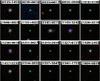 |
Fig. 10 20′′ × 20′′ SDSS composite g,r,i images of galaxies with m(3.4 μm)−m(4.6 μm) ≥ 2 mag. |
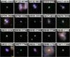 |
Fig. 11 20′′ × 20′′ SDSS composite g,r,i images of galaxies with 2 mag >m(3.4 μm)−m(4.6 μm) ≥ 1.5 mag. |
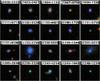 |
Fig. 11 continued. |
 |
Fig. 11 continued. |
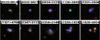 |
Fig. 12 20′′ × 20′′ SDSS composite g,r,i images of ten representative galaxies with m(3.4 μm)−m(4.6 μm) < 0.5 mag. |
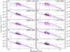 |
Fig. 13 Spectral energy distributions galaxies with m(3.4 μm)−m(4.6 μm) ≥ 2 mag. Observed SDSS optical spectra are shown by black solid lines; observed GALEX, SDSS and WISE monochromatic fluxes are shown by filled red circles. The WISE data are connected by a red solid line. The modelled SED shown by the blue line is a sum of stellar emission (green line) and ionised gas emission (magenta line). |
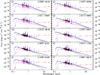 |
Fig. 13 continued. |
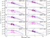 |
Fig. 14 continued. |
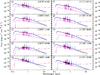 |
Fig. 14 continued. |
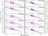 |
Fig. 14 continued. |
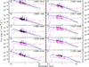 |
Fig. 14 continued. |
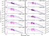 |
Fig. 14 continued. |
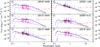 |
Fig. 14 continued. |
IRAF is the Image Reduction and Analysis Facility distributed by the National Optical Astronomy Observatory, which is operated by the Association of Universities for Research in Astronomy (AURA) under cooperative agreement with the National Science Foundation (NSF).
Acknowledgments
Y.I.I., N.G.G. and K.J.F. are grateful to the staff of the Max Planck Institute for Radioastronomy (MPIfR) for their warm hospitality. Y.I.I. and N.G.G. acknowledge financial support by the MPIfR. GALEX is a NASA mission managed by the Jet Propulsion Laboratory. This publication makes use of data products from the Two Micron All Sky Survey, which is a joint project of the University of Massachusetts and the Infrared Processing and Analysis Center/California Institute of Technology, funded by the National Aeronautics and Space Administration and the National Science Foundation. This publication makes use of data products from the Wide-field Infrared Survey Explorer, which is a joint project of the University of California, Los Angeles, and the Jet Propulsion Laboratory, California Institute of Technology, funded by the National Aeronautics and Space Administration. Funding for the Sloan Digital Sky Survey (SDSS) and SDSS-II has been provided by the Alfred P. Sloan Foundation, the Participating Institutions, the National Science Foundation, the US Department of Energy, the National Aeronautics and Space Administration, the Japanese Monbukagakusho, the Max Planck Society, and the Higher Education Funding Council for England. This research has made use of the NASA/IPAC Extragalactic Database (NED) which is operated by the Jet Propulsion Laboratory, California Institute of Technology, under contract with the National Aeronautics and Space Administration.
References
- Abazajian, K. N., Adelman-McCarthy, J. K., Agüeros, M. A., et al. 2009, ApJS, 182, 543 [NASA ADS] [CrossRef] [Google Scholar]
- Aller, L. H. 1984, Physics of Thermal Gaseous Nebulae (Dordrecht: Reidel) [Google Scholar]
- Andrews, B. H., & Martini, P. 2013, ApJ, 765, 140 [NASA ADS] [CrossRef] [Google Scholar]
- Baldwin, J. A., Phillips, M. M., & Terlevich, R. 1981, PASP, 93, 5 [NASA ADS] [CrossRef] [EDP Sciences] [Google Scholar]
- Calzetti, D., Armus, L., Bohlin, R. C., Kinney, A. L., & Storchi-Bergmann, T. 2000, ApJ, 533, 682 [NASA ADS] [CrossRef] [Google Scholar]
- Cardamone, C., Schawinski, K., Sarzi, M., et al., 2009, MNRAS, 399, 1191 [NASA ADS] [CrossRef] [Google Scholar]
- Cardelli, J. A., Clayton, G. C., & Mathis, J. S. 1989, ApJ, 345, 245 [NASA ADS] [CrossRef] [Google Scholar]
- Cohen, M., Wheaton, Wm. A., & Megeath, S. T. 2003, AJ, 126, 1090 [NASA ADS] [CrossRef] [Google Scholar]
- Condon, J. J., Cotton, W. D., Greisen, E. W., et al. 1998, AJ, 115, 1693 [NASA ADS] [CrossRef] [Google Scholar]
- Cresci, G., Hicks, E. K. S., Genzel, R., et al. 2009, ApJ, 697, 115 [NASA ADS] [CrossRef] [Google Scholar]
- Engelbracht, C. W., Rieke, G. H., Gordon, K. D., et al. 2008, ApJ, 678, 804 [NASA ADS] [CrossRef] [Google Scholar]
- Erb, D. K., Pettini, M., Shapley, A. E., et al. 2010, ApJ, 719,1168 [NASA ADS] [CrossRef] [Google Scholar]
- Epinat, B., Amram, P., Contini, T., et al. 2012, A&A, 539, 92 [Google Scholar]
- Ferland, G. 1980, PASP, 92, 596 [NASA ADS] [CrossRef] [Google Scholar]
- Fioc, M., & Rocca-Volmerange, B. 1997, A&A, 326, 950 [NASA ADS] [Google Scholar]
- FörsterSchreiber, N. M., Genzel, R., Bouché, N., et al. 2009, ApJ, 706, 1364 [NASA ADS] [CrossRef] [Google Scholar]
- Fukugita, M., Ichikawa, T., Gunn, J. E., et al. 1996, AJ, 111, 1748 [NASA ADS] [CrossRef] [Google Scholar]
- Girardi, L., Bressan, A., Bertelli, G., & Chiosi, C. 2000, A&AS, 141, 371 [NASA ADS] [CrossRef] [EDP Sciences] [Google Scholar]
- Gonçalves, T. S., Basu-Zych, A., Overzier, R., et al. 2010, ApJ, 724, 1373 [NASA ADS] [CrossRef] [Google Scholar]
- Griffith, R. L., Tsai, C.-W., Stern, D., et al. 2011, ApJ, 736, L22 [NASA ADS] [CrossRef] [Google Scholar]
- Guseva, N. G., Izotov, Y. I., & Thuan, T. X. 2006, ApJ, 644, 890 [NASA ADS] [CrossRef] [Google Scholar]
- Guseva, N. G., Izotov, Y. I., Papaderos, P., & Fricke, K. J. 2007, A&A, 464, 885 [NASA ADS] [CrossRef] [EDP Sciences] [Google Scholar]
- Guseva, N. G., Papaderos, P., Meyer, H. T., Izotov, Y. I., & Fricke, K. J. 2009, A&A, 505, 63 [NASA ADS] [CrossRef] [EDP Sciences] [Google Scholar]
- Heckman, T. M., Hoopes, C. G., Seibert, M., et al. 2005, ApJ, 619, L35 [NASA ADS] [CrossRef] [Google Scholar]
- Houck, J. R., Charmandaris, V., Brandl, B. R., et al. 2004, ApJS, 154, 211 [NASA ADS] [CrossRef] [EDP Sciences] [Google Scholar]
- Hoyos, C., Koo, D. C., Phillips, A. C., Willmer, C. N. A., & Guhathakurta, P. 2005, ApJ, 635, L21 [NASA ADS] [CrossRef] [Google Scholar]
- Hunt, L. K., Thuan, T. X., Izotov, Y. I., & Sauvage, M. 2010, ApJ, 712, 164 [NASA ADS] [CrossRef] [Google Scholar]
- Hunt, L. K., Magrini, L., Galli, D., et al. 2012, MNRAS, 427, 906 [NASA ADS] [CrossRef] [Google Scholar]
- Izotov, Y. I., & Thuan, T. X. 2007, ApJ, 665, 1115 [NASA ADS] [CrossRef] [Google Scholar]
- Izotov, Y. I., Thuan, T. X., & Lipovetsky, V. A. 1994, ApJ, 435, 647 [NASA ADS] [CrossRef] [Google Scholar]
- Izotov, Y. I., Thuan, T. X., & Lipovetsky, V. A. 1997, ApJS, 108, 1 [NASA ADS] [CrossRef] [Google Scholar]
- Izotov, Y. I., Stasińska, G., Meynet, G., Guseva, N. G., & Thuan, T. X. 2006, A&A, 448, 955 [NASA ADS] [CrossRef] [EDP Sciences] [Google Scholar]
- Izotov, Y. I., Guseva, N. G., & Thuan, T. X. 2011a, ApJ, 728, 161 [NASA ADS] [CrossRef] [Google Scholar]
- Izotov, Y. I., Guseva, N. G., Fricke, K. J., & Henkel, C. 2011b, A&A, 536, L7 [NASA ADS] [CrossRef] [EDP Sciences] [Google Scholar]
- Izotov, Y. I., Thuan, T. X., & Guseva, N. G. 2012, A&A, 546, A122 [NASA ADS] [CrossRef] [EDP Sciences] [Google Scholar]
- Kakazu, Y., Cowie, L. L., & Hu, E. M. 2007, ApJ, 668, 853 [NASA ADS] [CrossRef] [Google Scholar]
- Kauffmann, G., Heckman, T. M., Tremonti, C., et al. 2003, MNRAS, 346, 1055 [Google Scholar]
- Kennicutt, R. C. Jr., 1998, ARA&A, 36, 189 [Google Scholar]
- Lara-López, M. A., Cepa, J., Bongiovanni, A., et al. 2010, A&A, 521, L53 [NASA ADS] [CrossRef] [EDP Sciences] [Google Scholar]
- Leitherer, C. 1990, ApJS, 73, 1 [NASA ADS] [CrossRef] [Google Scholar]
- Manucci, F., Cresci, G., Maiolino, R., Marconi, A., & Gnerucci, A. 2010, MNRAS, 408, 2115 [NASA ADS] [CrossRef] [Google Scholar]
- Morrissey, P., Conrow, T., Barlow, T. A., et al. 2007, ApJS, 173, 682 [NASA ADS] [CrossRef] [Google Scholar]
- Pettini, M., Shapley, A. E., Steidel, C. C., et al. 2001, ApJ, 554, 981 [NASA ADS] [CrossRef] [Google Scholar]
- Planck collaboration 2013, A&A, in press [arXiv:1303.5075] [Google Scholar]
- Refsdal, S., Stabell, R., & de Lange, F. G., 1967, Mem. RAS, 71, 143 [NASA ADS] [Google Scholar]
- Schaerer, D., & de Barros, S. 2010, A&A, 515, 73 [Google Scholar]
- Schneider, D. P., Richards, G. T., Hall, P. B., et al. 2010, AJ, 139, 2360 [NASA ADS] [CrossRef] [Google Scholar]
- Skrutskie, M. F., Cutri, R. M., Stiening, R., et al. 2006, AJ, 131, 1163 [NASA ADS] [CrossRef] [Google Scholar]
- Stark, D. P., Ellis, R. S., Bunker, A., et al. 2009, ApJ, 697, 1493 [NASA ADS] [CrossRef] [Google Scholar]
- Stasińska, G., & Izotov, Y. I. 2003, A&A, 397, 71 [NASA ADS] [CrossRef] [EDP Sciences] [Google Scholar]
- Thuan, T. X., Izotov, Y. I., & Lipovetsky, V. A. 1995, ApJ, 445, 108 [NASA ADS] [CrossRef] [Google Scholar]
- Thuan, T. X., Sauvage, M., & Madden, S. 1999, ApJ, 516, 783 [NASA ADS] [CrossRef] [Google Scholar]
- Tremonti, C., Heckman, T. M., Kauffmann, G., et al. 2004, ApJ, 613, 898 [NASA ADS] [CrossRef] [Google Scholar]
- Wright, E. L., Eisenhardt, P. R. M., Mainzer, A. K., et al. 2010, AJ, 140, 1868 [NASA ADS] [CrossRef] [Google Scholar]
All Tables
All Figures
|
Fig. 1 Baldwin-Phillips-Terlevich (BPT) diagram (Baldwin et al. 1981). Selected SDSS star-forming galaxies are shown by blue filled circles. Also plotted are all emission-line galaxies from SDSS DR7 (cloud of grey dots). The red solid line from Kauffmann et al. (2003) separates star-forming galaxies from AGNs. |
| In the text | |
|
Fig. 2 Relation between the difference of oxygen abundances Δlog(O/H) derived by the direct and semi-empirical methods (Izotov & Thuan 2007) and the oxygen abundance obtained by the direct method. Only galaxies where [O iii] λ4363 is measured with accuracy better than 50% are shown. |
| In the text | |
|
Fig. 3 Distribution of the SDSS emission-line galaxies a) over redshift z; b) over extinction-corrected absolute- SDSS g-magnitude Mg; c) over total stellar mass M∗; d) over mass My of the young stellar population; e) over the extinction coefficient C(Hβ); f) over the equivalent width EW(Hβ) of the Hβ emission line; g) over the extinction- and aperture-corrected Hβ luminosity L(Hβ) (lower axis) and the star-formation rate SFR (upper axis); and h) over the oxygen abundance 12 +log O/H (h). Dotted vertical lines in all panels indicate mean values of the distributions. |
| In the text | |
|
Fig. 4 Relations between the extinction- and aperture-corrected Hβ luminosity L(Hβ) (abscissa) and different extinction-corrected luminosity ratios (ordinates). a) The GALEX FUV-to-Hβ luminosity ratio νLν(0.15 μm)/L(Hβ) is shown. Galaxies with EW(Hβ) ≥ 50 Å and EW(Hβ) < 50 Å are shown by red and blue symbols, respectively. The galaxies with red WISE W1 − W2 ≥ 2 mag colours are shown by large filled circles. b) Same as in a) but the GALEX NUV-to-Hβ luminosity ratio νLν(0.23 μm)/L(Hβ) is shown. c) Same as in a) but the SDSS u-to-Hβ luminosity ratio νLν(0.35 μm)/L(Hβ) is shown. d) Same as in a) but the SDSS g-to-Hβ luminosity ratio νLν(0.48 μm)/L(Hβ) is shown. e) Same as in a) but the SDSS r-to-Hβ luminosity ratio νLν(0.63 μm)/L(Hβ) is shown. f) Same as in a) but the SDSS i-to-Hβ luminosity ratio νLν(0.77 μm)/L(Hβ) is shown. g) Same as in a) but the SDSS z-to-Hβ luminosity ratio νLν(0.91 μm)/L(Hβ) is shown. h) Same as in a) but the 2MASS J-to-Hβ luminosity ratio νLν(1.24 μm)/L(Hβ) is shown. i) Same as in a) but the 2MASS H-to-Hβ luminosity ratio νLν(1.66 μm)/L(Hβ) is shown. j) Same as in a) but the 2MASS K-to-Hβ luminosity ratio νLν(2.16 μm)/L(Hβ) is shown. k) Same as in a) but the WISE W1-to-Hβ luminosity ratio νLν(3.4 μm)/L(Hβ) is shown. l) Same as in a) but the WISE W2-to-Hβ luminosity ratio νLν(4.6 μm)/L(Hβ) is shown. m) Same as in a) but the WISE W3-to-Hβ luminosity ratio νLν(12 μm)/L(Hβ) is shown. n) Same as in a) but the WISE W4-to-Hβ luminosity ratio νLν(22 μm)/L(Hβ) is shown. o) Same as in a) but the IRAS 60 μm-to-Hβ luminosity ratio νLν(60 μm)/L(Hβ) is shown. p) Same as in a) but the NVSS 20 cm-to-Hβ luminosity ratio νLν(20 cm)/L(Hβ) is shown. |
| In the text | |
|
Fig. 4 continued. |
| In the text | |
|
Fig. 5 Luminosity-metallicity relation. Symbols are the same as in Fig. 4. Linear likelihood regression is shown by solid line. Only 567 galaxies where the errors in [O iii] 4363 emission-line flux do not exceed 25% are also shown. The galaxies with red WISE colours W1 − W2 ≥ 2 mag are indicated by large black filled circles and the galaxies with SFR(Hα) ≥ 10 M⊙ yr-1 are encircled. |
| In the text | |
|
Fig. 6 a) Mass-metallicity relation. Symbols are the same as in Fig. 4. The linear likelihood regression is shown by solid line. The sample of galaxies is the same as in Fig. 5. The galaxies with red WISE colours W1 − W2 ≥ 2 mag are indicated by large black filled circles and the galaxies with SFR(Hα) ≥ 10 M⊙ yr-1 are encircled. For comparison, the mass-metallicity relation for 53 000 SDSS star-forming galaxies (Tremonti et al. 2004) is shown by a dashed line. b) Relation between the mass of the young stellar population and the oxygen abundance. The linear likelihood regression is shown by solid line. The galaxies with red WISE colours W1 − W2 ≥ 2 mag are resembled by large black filled circles and the galaxies with SFR(Hα) ≥ 10 M⊙ yr-1 are encircled. |
| In the text | |
|
Fig. 7 a)m(3.4 μm)− m(4.6 μm) vs. m(4.6 μm)−m(12 μm) colour–colour diagram for a sample of emission-line galaxies detected in the three WISE bands 3.4 μm (W1), 4.6 μm (W2), and 12 μm (W3). Galaxies with Hβ equivalent width EW(Hβ) ≥ 50 Å are shown by magenta filled circles while galaxies with EW(Hβ) < 50 Å are shown by cyan open circles. Twenty newly identified galaxies with m(3.4 μm)−m(4.6 μm) ≥ 2 mag are shown by large black filled circles. b) Same as in a) but galaxies with Hβ luminosity L(Hβ) ≥ 3 × 1040 erg s-1 are shown by orange filled circles while galaxies with L(Hβ) < 3 × 1040 erg s-1 are shown by green open circles. c) Same as in a) but galaxies with Hβ luminosity L(Hβ) ≥ 3 × 1040 erg s-1 and with Hβ equivalent width EW(Hβ) ≥ 50 Å are shown by red filled circles while galaxies with L(Hβ) < 3 × 1040 erg s-1 and with EW(Hβ) < 50 Å are shown by blue open circles. For comparison, gray dots in (c) show the location of QSOs selected in the SDSS. |
| In the text | |
|
Fig. 8 m(3.4 μm)−m(22 μm) vs. m(FUV)−r colour–colour diagram for a sample of emission-line galaxies detected in the WISE 3.4 μm (W1) and 22 μm (W4) bands and in the GALEX FUV band. Galaxies with Hβ equivalent width EW(Hβ) ≥ 50 Å and with L(Hβ) ≥ 3 × 1040 erg s-1 are shown by red filled circles, while galaxies with EW(Hβ) < 50 Å and with L(Hβ) < 3 × 1040 erg s-1 are depicted by blue open circles. Galaxies with m(3.4 μm)−m(4.6 μm)≥ 2 mag are shown by large black filled circles. |
| In the text | |
|
Fig. 9 m(3.4 μm)−m(4.6 μm) vs. 12 +log O/H diagram for a sample of emission-line galaxies detected in WISE 3.4 μm (W1) and 4.6 μm (W2) bands. Galaxies with Hβ equivalent width EW(Hβ) ≥ 50 Å and with L(Hβ) ≥ 3 × 1040 erg s-1 are shown by red filled circles while galaxies with EW(Hβ) < 50 Å and with L(Hβ) < 3 × 1040 erg s-1 are shown by blue open circles. Galaxies with m(3.4 μm)−m(4.6 μm)≥ 2 mag from this paper are shown by large black filled circles and from Griffith et al. (2011) by asterisks. Only the galaxies where the errors in [O iii] λ4363 emission-line flux do not exceed 50% are shown. |
| In the text | |
|
Fig. 16 a) Dependence of the luminosity L(WISE) integrated over all WISE bands in the wavelength range 3.4 μm−22 μm on the total extinction-corrected luminosity L(total) in the wavelength range 0.1 μm−22 μm. Galaxies with EW(Hβ) ≥ 50 Å and EW(Hβ) < 50 Å are shown by red and blue symbols, respectively. Galaxies with m(3.4 μm)−m(4.6 μm) ≥1.5 mag are shown by large black filled circles. Solid line is the line of equal values; dotted and dashed lines are maximum likelihood fits to the sample galaxies with EW(Hβ) ≥ 50 Å and EW(Hβ) < 50 Å, respectively. Error bars are average dispersions of the data around the fits. b) Dependence of the luminosity L(WISE) on the luminosity L(absorbed) of the absorbed emission in the wavelength range 0.1 μm−3 μm. The meaning of lines and symbols is the same as in a). |
| In the text | |
|
Fig. 17 Ratio L(WISE)/νLν(60 μm) vs. WISE W1 − W2 colour for the compact galaxies from the SDSS sample. Galaxies with L(Hβ) ≥ 3 × 1040 erg s-1 and L(Hβ) < 3 × 1040 erg s-1 are shown by red and blue dots, respectively. Galaxies with W1 − W2 ≥ 1.5 mag are shown by large black filled circles. |
| In the text | |
|
Fig. 10 20′′ × 20′′ SDSS composite g,r,i images of galaxies with m(3.4 μm)−m(4.6 μm) ≥ 2 mag. |
| In the text | |
|
Fig. 11 20′′ × 20′′ SDSS composite g,r,i images of galaxies with 2 mag >m(3.4 μm)−m(4.6 μm) ≥ 1.5 mag. |
| In the text | |
|
Fig. 11 continued. |
| In the text | |
|
Fig. 11 continued. |
| In the text | |
|
Fig. 12 20′′ × 20′′ SDSS composite g,r,i images of ten representative galaxies with m(3.4 μm)−m(4.6 μm) < 0.5 mag. |
| In the text | |
|
Fig. 13 Spectral energy distributions galaxies with m(3.4 μm)−m(4.6 μm) ≥ 2 mag. Observed SDSS optical spectra are shown by black solid lines; observed GALEX, SDSS and WISE monochromatic fluxes are shown by filled red circles. The WISE data are connected by a red solid line. The modelled SED shown by the blue line is a sum of stellar emission (green line) and ionised gas emission (magenta line). |
| In the text | |
|
Fig. 13 continued. |
| In the text | |
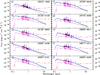 |
Fig. 14 Same as in Fig. 13 but for galaxies with 2 mag >m(3.4 μm)−m(4.6 μm) ≥ 1.5 mag. |
| In the text | |
|
Fig. 14 continued. |
| In the text | |
|
Fig. 14 continued. |
| In the text | |
|
Fig. 14 continued. |
| In the text | |
|
Fig. 14 continued. |
| In the text | |
|
Fig. 14 continued. |
| In the text | |
|
Fig. 14 continued. |
| In the text | |
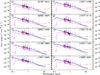 |
Fig. 15 Same as in Fig. 13 but for galaxies with m(3.4 μm)−m(4.6 μm) < 0.5 mag. |
| In the text | |
Current usage metrics show cumulative count of Article Views (full-text article views including HTML views, PDF and ePub downloads, according to the available data) and Abstracts Views on Vision4Press platform.
Data correspond to usage on the plateform after 2015. The current usage metrics is available 48-96 hours after online publication and is updated daily on week days.
Initial download of the metrics may take a while.