| Issue |
A&A
Volume 560, December 2013
|
|
|---|---|---|
| Article Number | A39 | |
| Number of page(s) | 16 | |
| Section | Interstellar and circumstellar matter | |
| DOI | https://doi.org/10.1051/0004-6361/201322400 | |
| Published online | 03 December 2013 | |
Deuterated water in the solar-type protostars NGC 1333 IRAS 4A and IRAS 4B⋆,⋆⋆
1 Université de Toulouse, UPS-OMP, IRAP, Toulouse, France
e-mail: This email address is being protected from spambots. You need JavaScript enabled to view it.
2 CNRS, IRAP, 9 Av. Colonel Roche, BP 44346, 31028 Toulouse Cedex 4, France
3 Niels Bohr Institute, University of Copenhagen, Juliane Maries Vej 30, 2100 Copenhagen Ø., Denmark
4 Centre for Star and Planet Formation, Natural History Museum of Denmark, University of Copenhagen, Øster Voldgade 57, 1350 Copenhagen K., Denmark
5 LERMA, Observatoire de Paris, UMR 8112 CNRS/INSU, 61 Av. de l’Observatoire, 75014 Paris, France
6 INAF – Osservatorio Astrofisico di Arcetri, Largo E. Fermi 5, 50125 Firenze, Italy
7 Harvard-Smithsonian Center for Astrophysics, 60 Garden Street, Cambridge, MA 02138, USA
8 Institut de Planétologie et d’Astrophysique de Grenoble (IPAG), UMR 5274, UJF-Grenoble 1/CNRS, 38041 Grenoble, France
9 Leiden Observatory, Leiden University, PO Box 9513, 2300 RA Leiden, The Netherlands
10 Max-Planck-Institut für Extraterrestrische Physik, Giessenbachstrasse 1, 85748 Garching, Germany
11 California Institute of Technology, Infrared Processing and Analysis Center, Mail Code 100-22, Pasadena, CA 91125, USA
12 Université de Bordeaux, Laboratoire d’Astrophysique de Bordeaux, 33000 Bordeaux, France
13 CNRS/INSU, UMR 5804, BP 89, 33271 Floirac Cedex, France
14 Physikalisches Institut, Universität zu Köln, Zülpicher Str. 77, 50937 Köln, Germany
15 Max-Planck-Institut für Radioastronomie, Auf dem Hügel 69, 53121 Bonn, Germany
16 University of Waterloo, Department of Physics and Astronomy, Waterloo, Ontario, Canada
17 NASA Postdoctoral Program Fellow, NASA Goddard Space Flight Center, 8800 Greenbelt Road, Greenbelt, MD 20770, USA
18 SRON Netherlands Institute for Space Research, Landleven 12, 9747 AD Groningen, The Netherlands
19 Kapteyn Astronomical Institute, University of Groningen, 9700 AV Groningen, The Netherlands
20 Department of Astronomy, University of Michigan, 500 Church Street, Ann Arbor, MI 48109-1042, USA
Received: 30 July 2013
Accepted: 21 October 2013
Abstract
Context. The measure of the water deuterium fractionation is a relevant tool for understanding mechanisms of water formation and evolution from the prestellar phase to the formation of planets and comets.
Aims. The aim of this paper is to study deuterated water in the solar-type protostars NGC 1333 IRAS 4A and IRAS 4B, to compare their HDO abundance distributions with other star-forming regions, and to constrain their HDO/H2O abundance ratios.
Methods. Using the Herschel/HIFI instrument as well as ground-based telescopes, we observed several HDO lines covering a large excitation range (Eup/k = 22–168 K) towards these protostars and an outflow position. Non-local thermal equilibrium radiative transfer codes were then used to determine the HDO abundance profiles in these sources.
Results. The HDO fundamental line profiles show a very broad component, tracing the molecular outflows, in addition to a narrower emission component and a narrow absorbing component. In the protostellar envelope of NGC 1333 IRAS 4A, the HDO inner (T ≥ 100 K) and outer (T < 100 K) abundances with respect to H2 are estimated with a 3σ uncertainty at 7.5-3.0+3.5 × 10⁻⁹ and 1.2-0.4+0.4 × 10⁻¹¹, respectively, whereas in NGC 1333 IRAS 4B they are 1-0.9+1.8 × 10⁻⁸ and 1.2-0.4+0.6 × 10⁻¹⁰, respectively. Similarly to the low-mass protostar IRAS 16293-2422, an absorbing outer layer with an enhanced abundance of deuterated water is required to reproduce the absorbing components seen in the fundamental lines at 465 and 894 GHz in both sources. This water-rich layer is probably extended enough to encompass the two sources, as well as parts of the outflows. In the outflows emanating from NGC 1333 IRAS 4A, the HDO column density is estimated at about (2–4) × 1013 cm-2, leading to an abundance of about (0.7–1.9) × 10-9. An HDO/H2O ratio between 7 × 10⁻⁴ and 9 × 10⁻² is also derived in the outflows. In the warm inner regions of these two sources, we estimate the HDO/H2O ratios at about 1 × 10⁻⁴–4 × 10⁻³. This ratio seems higher (a few %) in the cold envelope of IRAS 4A, whose possible origin is discussed in relation to formation processes of HDO and H2O.
Conclusions. In low-mass protostars, the HDO outer abundances range in a small interval, between ~10-11 and a few 10-10. No clear trends are found between the HDO abundance and various source parameters (Lbol, Lsmm, Lsmm/Lbol, Tbol, Lbol0.6/Menv). A tentative correlation is observed, however, between the ratio of the inner and outer abundances with the submillimeter luminosity.
Key words: astrochemistry / ISM: individual objects: NGC 1333 IRAS 4A / ISM: individual objects: NGC 1333 IRAS 4B / ISM: abundances / ISM: molecules
Based on observations carried out with the Herschel/HIFI instrument, the Institut de Radioastronomie Millimétrique (IRAM) 30 m Telescope, the James Clerk Maxwell Telescope (JCMT), and one of the ESO telescopes at the La Silla Paranal, the Atacama Pathfinder Experiment (APEX, programme ID 090.C-0239). Herschel is an ESA space observatory with science instruments provided by European-led principal Investigator consortia and with important participation from NASA. IRAM is supported by INSU/CNRS (France), MPG (Germany), and IGN (Spain). The JCMT is operated by the Joint Astronomy Centre on behalf of the Science and Technology Facilities Council of the United Kingdom, the Netherlands Organization for Scientific Research, and the National Research Council of Canada. APEX is a collaboration between the Max-Planck-Institut für Radioastronomie, the ESO, and the Onsala Space Observatory.
Appendices are available in electronic form at http://www.aanda.org
© ESO, 2013
1. Introduction
The study of the deuterated isotopologues of water, HDO and D2O, is helpful in order to understand water chemistry in the interstellar medium. Indeed, the HDO/H2O1 ratio can be used to constrain the water formation conditions. Water can be formed by different mechanisms, both in the gas phase and on grain surfaces. In diffuse clouds, gas-phase ion-molecule reactions lead to the formation of the H3O+ ion, which can dissociatively recombine to form H2O (e.g., Dalgarno 1980; Jensen et al. 2000). Water can also form in the gas phase through the endothermic reaction of O with H2 to form OH, followed by the reaction between OH and H2 (e.g., Wagner & Graff 1987). Because of the endothermicity of the first reaction (~2000 K) and the high energy barrier of the second reaction (~2100 K), this mechanism is only important in regions with high temperatures (>230 K), such as hot cores and shocks (Ceccarelli et al. 1996; Hollenbach & McKee 1979). In cold and dense regions, water is mainly formed by grain-surface chemistry, through hydrogenation of atomic and molecular oxygen accreted on the grains (e.g., Tielens & Hagen 1982; Ioppolo et al. 2008; Miyauchi et al. 2008; Dulieu et al. 2010; Cazaux et al. 2010). Water can then be thermally desorbed when the temperature is higher than ~100 K (Fraser et al. 2001), for example in the inner parts of the low-mass protostellar envelopes. It can also be released into the gas phase by non-thermal desorption mechanisms such as mechanical erosion (sputtering) in shocks (e.g., Flower & Pineau des Forêts 1994), or photodesorption by the interstellar radiation field or the cosmic ray induced UV-field (e.g., Öberg et al. 2009; Caselli et al. 2012). Deuterated water is expected to be formed in a similar way, but because of deuterium fractionation effects (e.g., Phillips & Vastel 2003), the HDO/H2O ratio is dependent on the temperature at which the water formation takes place. This ratio should then be high if water forms at low temperatures, whereas it should be low if water forms at high temperatures.
Parameters for the observed HDO lines.
In the past decade, many attempts have been made to explain the origin of Earth’s water. Its formation may be endogenous or exogenous: water adsorbed on dry silicate grains in the protosolar nebula (Stimpfl et al. 2004), delivery through asteroids, comets, planetary embryos, and planetesimals (Morbidelli et al. 2000; O’Brien et al. 2006; Raymond et al. 2004, 2006, 2009; Lunine et al. 2003; Drake & Campins 2006), and water production through oxidation of a hydrogen rich atmosphere (Ikoma & Genda 2006). These sources can be investigated by studying the water D/H ratio. For example, the value toward eight Oort Cloud comets is, on average, twice that of the standard mean ocean water (SMOW, 1.56 × 10⁻⁴) and 12 times the value of the D/H ratio in the early solar nebula (~2.5 × 10⁻⁵; Niemann et al. 1996; Geiss & Gloeckler 1998). This difference led to the conclusion that comets were not the main source of the delivery of water to Earth (e.g., Bockelée-Morvan et al. 1998; Meier et al. 1998; Villanueva et al. 2009), although the original value of the D/H ratio of the Earth’s water is unknown, and it is unclear how that value changed during the geophysical and geochemical evolution of the Earth (Campins & Lauretta 2004; Genda & Ikoma 2008). Recently, the water D/H ratio was measured with the HIFI spectrometer (Heterodyne Instrument for Far Infrared; de Graauw et al. 2010) onboard the Herschel Space Observatory (Pilbratt et al. 2010) to 1.61 × 10⁻⁴ in the Jupiter-family comet 103P/Hartley2 (Hartogh et al. 2011), close to the isotopic ratio measured in the Earth’s oceans (1.5 × 10⁻⁴; Lecuyer et al. 1998). The determination of the HDO/H2O ratio at different stages of the star formation process is then a way to determine how water evolves from the cold prestellar phase to the formation of planets and comets.
Until now, the HDO/H2O ratio has been determined in four Class 0 protostars, corresponding to the main accretion phase. At this stage, the results are quite disparate. For example, in the warm inner regions (T > 100 K) of IRAS 16293-2422, Parise et al. (2005) and Coutens et al. (2012, 2013) estimated a warm HDO/H2O ratio2, at about a few percent, using single-dish observations, whereas Persson et al. (2013) found a much lower estimate (~9 × 10⁻⁴) using interferometric data. This source is not the only one to present divergent results that depend on the studies. Indeed, the HDO/H2O ratio in the warm inner envelope of NGC 1333 IRAS 2A, first estimated by Liu et al. (2011) at ≥1%, was determined at about 1 × 10⁻³ after revision of the H2O abundance by Visser et al. (2013). This result remains different from another estimate, (0.3–8) × 10-2, by Taquet et al. (2013a). In NGC 1333 IRAS 4A (hereafter IRAS 4A) and NGC 1333 IRAS 4B (hereafter IRAS 4B), fewer studies have been carried out and are only based on interferometric observations. In IRAS 4A, Taquet et al. (2013a) found a ratio of 5 × 10⁻³ − 3 × 10⁻², and in IRAS 4B, Jørgensen & van Dishoeck (2010a) derived an upper limit of ~6 × 10⁻⁴. For more details on the results of the different studies of HDO/H2O ratios in Class 0 sources and their type of analysis, we refer the reader to Table 4 and Sect. 4.2. Singly deuterated water has also been studied in ices. Only upper limits between 5 × 10⁻³ and 2 × 10⁻² have been determined (Parise et al. 2003; Dartois et al. 2003), which do not allow us to conclude on rather high (~10-2) or low (≲10-3) HDO/H2O ratios in grain mantles.
Even if it is not possible to disentangle the emission from the hot corino (defined as the warm inner part of the envelope in which complex organic species are detected; Bottinelli et al. 2004) and the outer envelope using single-dish telescopes, these observations can be extremely helpful to constrain the HDO/H2O ratio in the outer part of the protostellar envelopes (T < 100 K). Indeed, the extended emission coming from the cold envelope cannot be probed with interferometers. Only two Class 0 sources were consequently studied for their cold HDO/H2O ratios2. It was determined to be between 3 × 10⁻³ and 1.5 × 10⁻² in IRAS 16293-2422 by Coutens et al. (2012, 2013), and between 9 × 10⁻³ and 1.8 × 10⁻¹ in NGC 1333 IRAS 2A by Liu et al. (2011). The fundamental HDO 11,1–00,0 transition at 894 GHz observed with Herschel/HIFI at high sensitivity provides particularly strong constraints on the outer HDO abundance. In IRAS 16293-2422, this line shows a specific line profile with a very deep absorption in addition to emission (Coutens et al. 2012). Combined with the observation of the other fundamental HDO 10,1–00,0 transition at 465 GHz with the JCMT, Coutens et al. (2012) showed that a cold water-rich absorbing layer surrounds this source. Without this layer, the deep absorbing components cannot be reproduced. Similar conclusions were obtained for the D2O absorbing lines observed with Herschel (Vastel et al. 2010; Coutens et al. 2013). However, the origin of this absorbing layer is not clearly determined. It has been suggested, for example, that it could result from an equilibrium between photodesorption and photodissociation by the UV interstellar radiation field, as predicted by Hollenbach et al. (2009). It would thus be helpful to know if this layer is observed around other protostars. Indeed, the ubiquity of this layer would give clues to the nature of this layer.
A collaboration between three Herschel key programs: CHESS (Chemical HErschel Surveys of Star forming regions; Ceccarelli et al. 2010), WISH (Water In Star-forming regions with Herschel; van Dishoeck et al. 2011), and HEXOS (Herschel/HIFI observations of EXtraOrdinary Sources: The Orion and Sagittarius B2 Star-forming Regions; Bergin et al. 2010) was set up to investigate the water chemistry in star-forming regions. As part of this collaboration, new observations of HDO were carried out towards two low-mass protostars, IRAS 4A and IRAS 4B, allowing us to estimate the HDO abundance profiles in these sources. These results are useful to derive, in particular, the HDO/H2O ratio in the outer envelope of these protostars. These two sources are located in the NGC 1333 reflection nebula in the Perseus molecular cloud. They are separated by 31″ (~7500 AU), and IRAS 4A is a binary system with a separation of ~1.8″ between its two components (Lay et al. 1995; Jørgensen et al. 2007). These protostars are well known for the complex organic chemistry observed in their hot corinos (Bottinelli et al. 2004, 2007; Sakai et al. 2006; Persson et al. 2012) and for their outflows detected in particular in CO, SiO, and CS (see, e.g., Blake et al. 1995; Lefloch et al. 1998; Choi 2005; Yıldız et al. 2012) and in H2O (Kristensen et al. 2010, 2012). The distance to the NGC 1333 region is uncertain (see Curtis et al. 2010 for more details). We adopt here the distance of 235 ± 18 pc determined by Hirota et al. (2008) using very-long-baseline interferometry (VLBI) parallax measurements of water masers in SVS 13 located in the same cloud.
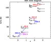 |
Fig. 1 Energy level diagram of the HDO lines. In red, IRAM-30 m observations; in magenta, JCMT/APEX observation; in blue, HIFI observations. The frequencies are written in GHz. |
The paper is organized as follows. First, we present the observations in Sect. 2. Then we describe the modeling and show the results in Sect. 3. Finally, we discuss the results in Sect. 4 and conclude in Sect. 5.
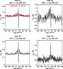 |
Fig. 2 Upper-left panel: HIFI observations of the fundamental line at 894 GHz towards the protostar IRAS 4A (black) and an outflow position (red, discussed in Sect. 3.3). The spectrum at the outflow position has been shifted vertically by 0.178 K. Upper-right panel: JCMT observations of the fundamental line at 465 GHz towards IRAS 4A. Lower-left panel: HIFI observations of the fundamental line at 894 GHz towards the protostar IRAS 4B. Lower-right panel: APEX observations of the fundamental line at 465 GHz towards IRAS 4B. The continuum refers to SSB data for each panel. |
HDO line components observed towards IRAS 4A and IRAS 4B.
2. Observations
The various transitions observed towards IRAS 4A and IRAS 4B are shown in the energy level diagram in Fig. 1 and summarized in Table 1. The original observations (without subtraction of the broad outflow component) of the 11,1–00,0 and 10,1–00,0 fundamental transitions are presented in Fig. 2. The other transitions are shown with the modeling in Figs. 5 and 7.
2.1. HIFI data
In the framework of a collaboration between the CHESS, WISH, and HEXOS Herschel key programs, two HDO transitions were observed with the HIFI instrument towards the solar-type protostars IRAS 4A and IRAS 4B: the fundamental 11,1–00,0 line at 894 GHz with Eup = 43 K, and the 21,1–20,2 line at 600 GHz with Eup = 95 K (see Table 1). The targeted coordinates are  , δ2000 = 31°13′30.9″ for IRAS 4A, and
  , δ2000 = 31°13′8.1″ for IRAS 4B. The two transitions were also observed in the red-shifted part of the outflow emanating from IRAS 4A at
  , δ2000 = 31°13′50.9″. It corresponds to an offset position (+4″, +20″) with respect to IRAS 4A. This position was chosen using the map of the CO 6–5 line in Fig. 3 of Yıldız et al. (2012), so that the telescope half power beam width (HPBW) at 600 and 894 GHz (36 and 24″, respectively) do not include the position of the IRAS 4A source.
The pointed observations were obtained in August 2011, using the HIFI double beam switch (DBS) fast chop mode with optimization of the continuum. The DBS reference positions were situated at 3′ from the source. We checked that no line was detected in the OFF-position spectra. The HIFI wide band spectrometer (WBS) was used, providing a spectral resolution of 1.1 MHz (0.55 km s-1 at 600 GHz and 0.37 km s-1 at 894 GHz). The data were processed using the standard HIFI pipeline up to frequency and amplitude calibrations (level 2) with the ESA-supported package HIPE 7.1 (Ott 2010). After being inspected separately, the H and V polarizations were averaged weighting them by the observed noise, using the GILDAS/CLASS3 software. The forward efficiency is about 0.96 and the main beam efficiency about 0.74–0.75 (Roelfsema et al. 2012). The HIFI instrument uses double sideband receivers. A sideband gain ratio of 1 is assumed to estimate the continuum value at 894 GHz (Roelfsema et al. 2012), necessary in the modeling of the deep absorption line. The continuum was fitted with a polynomial of degree 1. Standing waves are not visible in the observations. From Roelfsema et al. (2012), we thus estimate the uncertainties on the continuum level to be less than 10% for both IRAS 4A and IRAS 4B observations. Observations were also carried out with the high resolution spectrometer (HRS). The WBS and HRS observations are in agreement (see Fig. A.1).
The line profiles observed at 894 GHz clearly show a broad emission component tracing the outflows, a narrower emission component tracing the envelope, and a deep narrow absorption component (see Fig. 3). The parameters of the three components, fitted by Gaussians using the CASSIS4 software, are presented in Table 2. Figure 2 superposes the HIFI HDO spectra towards IRAS 4A and the position in the red outflow lobe. The spectrum in the red lobe is similar to that towards IRAS 4A except that the blue outflow wing is no longer seen. The absorption appears less deep because of the lower continuum level at the outflow position.
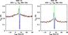 |
Fig. 3 Decomposition of the 11,1–00,0 fundamental transitions observed towards IRAS 4A and IRAS 4B with HIFI in three Gaussians: a broad emission component (red), a narrower emission component (green), and a narrow absorption component (blue). The parameters of the Gaussian fits are given in Table 2. |
2.2. JCMT data
The HDO 10,1–00,0 fundamental transition at 465 GHz (Table 1) was observed towards the source IRAS 4A with the JCMT in September 2004 (project M04BN06). The spectral resolution of the observations is 0.1 km s-1. As in the case of the other fundamental transition at 894 GHz observed with HIFI, three components are observed: a broad component tracing the outflows, a narrower emission line, and a deep absorption component (see Fig. 2). The continuum level is ~0.8 K with an uncertainty of 13% obtained from the comparison of the spectra in the dataset. The full width at half maximum (FWHM) and the peak-intensity velocity of the Gaussian fitted on the broad component at 894 GHz are consistent with the data at 465 GHz. The fit results from the higher signal-to-noise ratio profile at 894 GHz were then fixed for the 465 GHz profile to determine the intensity of the broad component (see Table 2). Keeping parameters free would not affect the results significantly.
2.3. APEX data
The HDO 10,1–00,0 fundamental transition was also observed towards IRAS 4B with the Swedish Heterodyne Facility Instrument (SHeFI) receiver at 460 GHz of the APEX telescope. The observations were carried out in October 2012 using the wobbler symmetric switching mode with an amplitude of 150″, resulting in OFF positions at 300″ from the source. The beam efficiency and the forward efficiency are shown in Table 1. This fundamental line again shows a broad emission component, a narrow emission component, and a weak absorbing component. The absorbing component appears weaker than in IRAS 4A, because the absorbing line is slightly shifted with respect to the velocity of the narrower emission component, leading to less absorption than there would be if the velocity of the absorption was exactly the same as the velocity of the emission. A continuum level cannot be extracted with precision from these observations. It is estimated at about 0.2 K according to the model predictions (see Sect. 3.2). The continuum level would then be lower in IRAS 4B than in IRAS 4A (~0.8 K), which also implies a shallower absorption in IRAS 4B for the same column density of the absorber.
2.4. IRAM data
Three additional transitions at 81 (11,0–11,1), 226 (31,2–22,1), and 242 GHz (21,1–21,2) were observed with the IRAM-30 m telescope towards IRAS 4A. The observations were carried out in November 2004 for the 81 and 226 GHz lines with the VESPA autocorrelator in wobbler switching mode, whereas the 242 GHz transition was observed in April 2012 in position switching mode using the fast Fourier transform spectrometer (FTS) at a 200 kHz resolution. The spectral resolution is 0.14, 0.10, and 0.24 km s-1 for the 81, 226, and 242 GHz transitions respectively. For clarity, the spectra shown hereafter were smoothed to a resolution of ~0.4–0.6 km s-1.
These three transitions were also observed towards IRAS 4B in January 2013. The observations were carried out in position switching mode using the FTS with a fine spectral resolution of 50 kHz. The beam efficiencies and forward efficiencies for the different observations are shown in Table 1.
Table 2 summarizes, for each line, the Gaussian parameters of the different components derived with CASSIS. The FWHM of the narrower emission component is different depending on the line. Indeed these sources undergo an infall which necessarily leads to higher FWHM for the excited lines, such as the 31,2–22,1 and 21,1–21,2 transitions that probe the warm inner regions, and smaller FWHM for the fundamental lines that probe a colder medium. Moreover, the determination of the FWHM for the fundamental lines could be underestimated because of the blending between the narrow emission and absorption components. Only the broad emission component can be clearly extracted thanks to the absence of blending at high velocities (Δν > 3 km s-1).
3. Modeling and results
3.1. Protostellar envelope of NGC 1333 IRAS 4A
The spherical non-LTE (local thermal equilibrium) radiative transfer code RATRAN (Hogerheijde & van der Tak 2000), which includes continuum emission and absorption by dust, was used to determine the HDO abundances in the protostellar envelope. First, it was necessary to subtract the broad outflow component fitted by a Gaussian profile (see Table 2) from the HDO fundamental transitions at 465 and 894 GHz. Then a similar method to the study on the protostar IRAS 16293-2422 (Coutens et al. 2012) was carried out on the line profiles obtained after the removal of the broad component. We used the HDO collisional rates calculated with ortho and para–H2 (Faure et al. 2011; Wiesenfeld et al. 2011), assuming an ortho/para ratio of H2 at local thermodynamic equilibrium with the gas temperature. The density and temperature radial profiles of the source IRAS 4A were determined by Kristensen et al. (2012). The envelope mass is estimated at 5.2 M⊙ (Kristensen et al. 2012), and the radius of the protostellar envelope extends from 33.5 AU to 33 500 AU. The density power-law index is 1.8. At r = 1000 AU, the density is equal to 6.7 × 106 cm-3, and the temperature is 21 K. However, at small scale (≲500 AU, Jørgensen et al. 2004), the structure is rather uncertain because of the limited spatial resolution of the continuum maps used to determine the profiles. The velocity profile is assumed as a free-fall profile ( ). The central mass M was estimated at ~0.5 M⊙ by Maret et al. (2002) and Jørgensen et al. (2009) and at ~0.7 M⊙ by Di Francesco et al. (2001) and Mottram et al. (2013). Several grids of models with different values of M (0.3, 0.5, and 0.7 M⊙) were then run. To reproduce the absorption component seen in the fundamental lines, the Doppler b-parameter (db), which is related to the turbulence broadening, is estimated at 0.4 km s-1. This is the same as found independently for H2O by Mottram et al. (2013). It means that the FWHM produced by the turbulence is equal to db/0.6, i.e., about 0.67 km s-1. The continuum is not correctly fitted with the dust opacity used by Kristensen et al. (2012, model OH5 in Ossenkopf & Henning 1994. It is 17% lower than the observed continuum at 465 GHz and 28% higher at 895 GHz. Calibration uncertainties could play a role. The study of the absorbing components requires, however, the use of the correct continuum value. A power-law emissivity model was then estimated locally to fit the observed continuum,
 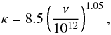 (1)with κ the absorption coefficient in cm2 g
 and ν the frequency in Hz. We assumed an abundance profile with a jump at 100 K (θ ~ 0.73″, r ~ 85 AU), for the release by thermal desorption of the water molecules trapped in the icy grain mantles into the gas phase (Fraser et al. 2001). This type of jump abundance profile was assumed in a number of studies of water and deuterated water in low-mass protostars (Ceccarelli et al. 2000; Parise et al. 2005; Liu et al. 2011; Coutens et al. 2012). A recent study shows, however, that in the outer envelope of low-mass protostars the H
 O line profiles are better reproduced with an abundance increasing gradually with radius (Mottram et al. 2013). To compare the HDO abundances in IRAS 4A with previous results in other low-mass protostars and to keep a reasonable number of free parameters in the modeling, we used a jump abundance profile with a constant outer abundance for this study.
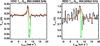 |
Fig. 4 Comparison of the modeling of the HDO 11,1–00,0 and 10,1–00,0 fundamental transitions observed towards IRAS 4A with an added absorbing layer (in green) and without this layer (in red). The HDO column density in the absorbing layer is about 1.4 × 1013 cm-3. The broad outflow component seen in the observations was subtracted. The continuum refers to SSB data. |
Grids of models with different inner (Xin) and outer (Xout) abundances5, and central masses (M) were run. Similarly to IRAS 16293-2422 (Coutens et al. 2012), an absorbing layer had to be added to the structure to reproduce the absorption lines observed at 894 and 465 GHz, without overpredicting the line emissions. Figure 4 shows the difference of the modeling with and without the absorbing layer for an HDO column density of 1.4 × 1013 cm-3. The analysis and the discussion regarding this layer are detailed in Sect. 3.3. A χ2 minimization was then used to determine the best-fit parameters, adding this absorbing layer to the structure. The χ2 is computed on the line profiles with the formalism, 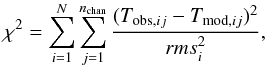 (2)with N the number of observed lines i, nchan the number of channels j for each line, Tobs,ij and Tmod,ij the intensity observed and predicted by the model in the channel j of the line i, and rmsi the rms of the line i. Taking into account this foreground absorbing layer in the modeling, the best-fit is obtained for an inner abundance Xin = 7.5 × 10⁻⁹, an outer abundance Xout = 1.2 × 10⁻¹¹, and a central mass M = 0.5 M⊙. The line profiles predicted by this model are shown in Fig. 5, and the χ2 contours at 1, 2, and 3σ are plotted in Fig. 6. At 3σ, the inner abundance is between 4.5 × 10⁻⁹ and 1.1 × 10⁻⁸, whereas the outer abundance is between 8 × 10-12 and 1.6 × 10⁻¹¹. Although the models with M = 0.3 M⊙ and M = 0.7 M⊙ show higher χ2 values, some of them are, however, included in the 3σ uncertainties. For these masses, the best-fit abundances remain quite similar: Xin = 7.0 × 10⁻⁹, Xout = 1.2 × 10⁻¹¹ for M = 0.3 M⊙ and Xin = 8.5 × 10⁻⁹, Xout = 1.0 × 10⁻¹¹ for M = 0.7 M⊙.
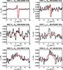 |
Fig. 5 In black: HDO lines observed towards IRAS 4A with HIFI, IRAM, and JCMT. The broad outflow component seen in the observations was subtracted. The continuum seen in the observations of the 894 GHz and 465 GHz lines refers to SSB data. In red: best-fit model obtained when adding an absorbing layer with an HDO column density of ~1.4 × 1013 cm-2 to the structure. The best-fit inner abundance is 7.5 × 10⁻⁹ and the best-fit outer abundance is 1.2 × 10⁻¹¹. |
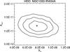 |
Fig. 6 χ2 contours at 1σ, 2σ, and 3σ obtained for IRAS 4A when adding an absorbing layer with an HDO column density of 1.4 × 1013 cm-2 to the structure. The best-fit model is represented by the symbol “+”. The mass is equal to 0.5 M⊙. |
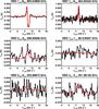 |
Fig. 7 In black: HDO lines observed towards IRAS 4B with HIFI, IRAM, and APEX. The broad outflow component seen in the observations was subtracted. The continuum seen in the observations of the 894 GHz and 465 GHz lines refers to SSB data. In red: best-fit model obtained when adding the absorbing layer used to model the IRAS 4A lines (N(HDO) ~ 1.4 × 1013 cm-2). The best-fit inner abundance is 1 × 10⁻⁸ and the best-fit outer abundance is 1.2 × 10⁻¹⁰. |
3.2. Protostellar envelope of NGC 1333 IRAS 4B
A similar modeling was carried out to determine the HDO abundance distribution in IRAS 4B. The outflow components were subtracted here again. We used the source structure determined by Kristensen et al. (2012), for which the radius of the protostellar envelope ranges between 15 AU and 12 000 AU and the envelope mass is about 3.0 M⊙. The density power-law index is 1.4. At r = 1000 AU, the density is 5.7 × 106 cm-3, and the temperature is 17 K. As in the case of IRAS 4A, the structure is quite uncertain at small scale. According to this structure, the size of the abundance jump (T > 100 K) is θ ~ 0.4″, i.e., r ~ 47 AU. When the absorbing layer defined for IRAS 4A (N(HDO) = 1.4 × 1013 cm-2) is added to the structure of its nearby companion IRAS 4B, the absorbing components are well reproduced (see Fig. 7). The velocity profile is assumed to be a free-fall profile. The central mass M derived in previous studies varies by more than a factor of 2. Di Francesco et al. (2001) and Jørgensen et al. (2009) predicted a mass about 0.2 M⊙, whereas Maret et al. (2002) determined a mass about 0.5 M⊙.
Several values were then considered for the central mass M chosen from 0.1 M⊙ to 0.5 M⊙ in steps of 0.1 M⊙. The Doppler b-parameter is estimated at 0.5 km s-1, to reproduce the deep absorbing component at 894 GHz. We used the emissivity model determined by Ossenkopf & Henning (1994), for thin ice-coated grains with a growth of 106 years (OH5, similar to Kristensen et al. 2012), which gives a dust continuum value in agreement with the Herschel/HIFI observations. The continuum level at 465 GHz is then predicted at about 0.2 K for the APEX beam.
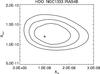 |
Fig. 8 χ2 contours at 1σ, 2σ, and 3σ obtained for IRAS 4B when adding the absorbing layer used to model the IRAS 4A lines. The best-fit model is represented by the symbol “+”. The mass is equal to 0.1 M⊙. |
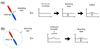 |
Fig. 9 Different scenarios for the position of the absorbing layer with respect to the protostar and the outflows and influence on the absorbing line depth. In case a), the absorbing layer is less extended than the outflows. The continuum that is absorbed is only due to the protostar. The broad component is superposed. In case b), the absorbing layer is more extended than the outflows. The continuum that is absorbed is due both to the protostar and the outflows. |
Running a grid with different values for Xin, Xout, and M, the best-fit model is obtained for an inner abundance of about 1 × 10⁻⁸, an outer abundance of about 1.2 × 10⁻¹⁰, and a central mass of about 0.1 M⊙. The best-fit line profiles are overplotted on the observations in Fig. 7. The χ2 contours are shown in Fig. 8. At 3σ, the inner abundance varies between 1.5 × 10⁻⁹ and 2.8 × 10⁻⁸, whereas the outer abundance is included between 8.5 × 10⁻¹¹ and 1.75 × 10⁻¹⁰. Some models with M = 0.2 M⊙ are also included in the 3σ uncertainties, but not for masses higher than or equal to 0.3 M⊙.
3.3. Absorbing layer
Depending on the position of the absorbing layer with respect to the outflows, the depth of the absorption components may vary after the subtraction of the broad component. Indeed, if the absorbing layer is situated between the outflows and the protostellar envelope (see case (a) in Fig. 9), the depth of the absorption line has to be unchanged after the subtraction of the large component, because the continuum produced by the outflows (i.e., the broad component) is not absorbed by the added layer. On the contrary, if the absorbing layer is located in front of the outflows (see case (b) in Fig. 9), the continuum obtained after subtraction is lower than the real absorbed continuum, since the line wing effectively contributes to the continuum that is being absorbed. In this case, to accurately estimate the HDO column density in the absorbing layer, the depths of the absorbing lines must be corrected, reducing them by a value close to the intensities of the broad components. The uncertainty on this value is ≲10%, which is comparable to the calibration uncertainties of the HIFI observations and is probably even lower for the JCMT observations. The presence of an absorption component in the data at 894 GHz towards the outflow of IRAS 4A (see Fig. 2) suggests that the foreground absorbing layer is more extended than a part of the outflows (case (b) in Fig. 9). When subtracting the broad components on the IRAS 4A observations, the depth of the absorbing lines was consequently reduced to take into account the absorption by the continuum produced by the outflows. We assumed a similar behavior for IRAS 4B and treated the absorptions in the same way.
To reproduce the depth of the absorption lines, the column density of HDO is then about 1.4 × 1013 cm-2. The temperature is assumed to be between 10 and 30 K and the H2 density is found to be lower than 105 cm-3 to reproduce the absorptions. This upper limit on the H2 density is consistent with the study by Coutens et al. (2013) using the D2O lines observed towards IRAS 16293-2422. The HDO column density derived here differs by less than a factor of 2 compared with the estimate in the absorbing layer of IRAS 16293-2422 (2.3 × 1013 cm-2; Coutens et al. 2012). As the absorbing layer shows the same characteristics for IRAS 4A and IRAS 4B, this could mean that this layer is sufficiently extended (≳7000 AU) to encompass the two sources.
Several molecules (CO, HCN, HCO+, H2CO) show, over a large extent (≳200″) around IRAS 4, asymmetric line-profiles with dips at a velocity about 8 km s-1 (~7.5 km s-1 at the IRAS 4A position; Choi et al. 2004). In our data, the velocity of the absorbing components appears at 7.6 km s-1. These molecules and water could consequently arise from the same absorbing layer. The origin of this absorbing layer was largely debated (e.g., Langer et al. 1996; Di Francesco et al. 2001; Choi 2001, and references therein). In particular, Choi et al. (2004) interpreted these absorptions as produced by a cold foreground layer unrelated to the IRAS 4A source. This interpretation was, however, questioned by Belloche et al. (2006), as they showed that an infall motion would be sufficient to explain the observed absorptions of CS and N2H+ transitions if a source velocity of 7.2 km s-1 is assumed instead of the value of 6.7 km s-1 used by Choi et al. (2004). Walsh et al. (2006) drew similar conclusions, favoring the interpretation that the HCO+ line profiles are indicative of large-scale inward motions associated with the IRAS4A source. In our study, nothing allows us to conclude that the water-rich absorbing layer is unrelated to the protostellar sources. This cold layer could consequently be a part of the complex surrounding IRAS 4.
While it is not surprising to detect molecules such as CO, HCO+, etc., in cold environments, the presence of water is more puzzling. Indeed, at low temperatures, water is mainly trapped on the grain mantles. Hypotheses were suggested by Coutens et al. (2012) to explain the presence of a water-rich absorbing layer surrounding the protostar IRAS 16293-2422. The most probable explanation is that this layer results from an equilibrium between the photodesorption of water molecules trapped in the icy grain mantles and their photodissociation by an external UV radiation field, as predicted by Hollenbach et al. (2009) in molecular clouds at a visual extinction AV between 1 and 4. Assuming the relation NH/AV = 2 × 1021 cm-2 mag-1 (Vuong et al. 2003), the deuterated water abundance with respect to H2 would then be ~3.7 × 10⁻⁹–1.5 × 10⁻⁸ in the assumed photodesorption layer of IRAS 4, which is comparable to the layer surrounding IRAS 16293-2422 (~6 × 10⁻⁹–2.4 × 10⁻⁸). Other mechanisms able to explain the presence of gaseous water in a cold layer are discussed in Appendix B.
We have to point out that photodesorption by the cosmic-ray induced UV-field certainly plays a role in the outer envelope, as shown by Mottram et al. (2013) in low-mass protostars and Caselli et al. (2012) in prestellar cores. In this case, the abundance increases gradually with the outer radius. As the outer abundance is assumed to be constant here, a part of the absorption could also be produced in the outermost part of the envelope (which encompasses the outflow position and shows low temperatures as well as low densities). The column density of water derived in the added absorbing layer should then be considered to be an upper limit. An analysis of the HDO lines with a more physical abundance profile in the outer layer would be required to know the proportion of cold water in the outer envelope and at larger scale in the molecular cloud.
HDO abundances with respect to H2 determined in several low-mass star-forming regions.
3.4. Outflow of NGC 1333 IRAS 4A
A broad component tracing the outflows is seen in the two fundamental 11,1–00,0 and 10,1–00,0 transitions observed with HIFI and JCMT towards IRAS 4A. This HDO outflow component is very similar to the broad component seen on the CO 6–5 line profile observed with APEX by Yıldız et al. (2012) (see Fig. 10), suggesting a common origin for the entrainment of the HDO and CO molecules. The RADEX non-LTE radiative transfer code (van der Tak et al. 2007) was employed to estimate the HDO column density present in the outflows of IRAS 4A. We used a H2 density of 3 × 105 cm-3 and a temperature between 100 and 150 K, as determined by Yıldız et al. (2012) for CO in the outflow positions R1 and B1. The HDO column density is estimated at ~(2–4) × 1013 cm-2. These estimates remain valid, even if the temperature is lower than 100 K. Using the H2 column density of (2.1–2.8) × 1022 cm-2 estimated by Yıldız et al. (2012) in the outflows, the HDO abundance is therefore about 7 × 10⁻¹⁰ − 1.9 × 10⁻⁹.
The HDO/H2O ratio in the outflows can be also estimated with RADEX using the line ratios of the HDO 11,1–00,0 line at 894 GHz with the para–H2O 11,1–00,0 line at 1113 GHz (Kristensen et al. 2010). At these frequencies, the beam sizes are quite similar (19″ vs. 24″). An ortho-to-para ratio of 3 is assumed to consider the H2O abundance. The profile of the para–H2O line appears quite different from that of the HDO line (see Fig. 10). The H2O outflow profile shows a peak intensity at − 0.6 km s-1 that we do not see for the HDO lines. Kristensen et al. (2010) fitted it with a sum of two Gaussians, one centered at − 0.6 km s-1 and a broader one centered at 8.7 km s-1. However, it is not possible to reproduce the HDO profile with the same velocity and FWHM. To estimate the HDO/H2O abundance ratio in the outflows, we consequently compared the predicted line ratios with the line ratios at the velocities where the HDO broad component is detected. A range of densities (105–107 cm-3) and temperatures (100–1000 K) was considered. The derived HDO/H2O ratio ranges between 1 × 10⁻³ and 9 × 10⁻² in the red part of the outflow and between 7 × 10⁻⁴ and 6 × 10⁻² in the blue part of the outflow. These estimates are consistent with the HDO/H2O ratio derived by Taquet et al. (2013a) in the hot corino of IRAS 4A (5 × 10⁻³–3 × 10⁻²). If the HDO/H2O ratios are actually similar in the outflow and in the hot corino, it could mean that water is contained in grain mantles and then released into the gas phase by sputtering in outflows and thermal desorption in the warm inner envelope. The isotopologue HDO would then be omnipresent and produced early in the evolution of the core. However, the wide range of values determined here does not allow us to clearly assert this possibility. The HDO/H2O ratio is not determined at high velocities (Δν > 10 km s-1) where only H2O is detected.
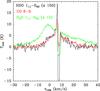 |
Fig. 10 Comparison of the line profiles of the CO 6–5 transition (in red), the HDO 11,1–00,0 transition (in black, intensities multiplied by 150), and the H2O 11,1–00,0 transition (in green, intensities multiplied by 15) towards IRAS 4A. |
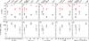 |
Fig. 11 Upper panels: comparison of the inner (red) and outer (black) HDO abundances estimated in the low-mass protostars IRAS 16293-2422, NGC 1333 IRAS 4A, NGC 1333 IRAS 2A, and L1448-mm (see also Table 3) as a function of a) the ratio between the submillimeter and bolometric luminosities Lsmm/Lbol; b) the bolometric luminosity Lbol; c) the submillimeter luminosity Lsmm; d) the bolometric temperature Tbol; e) the ratio |
4. Discussion
4.1. Comparison of the HDO abundances in low-mass star-forming regions
Table 3 summarizes the HDO abundances measured in low-mass protostars. For all sources except L1448-mm, the derived abundances are based on RATRAN modeling of multi-line single-dish observations. For IRAS 16293-2422, IRAS 4A, and IRAS 4B, the HDO fundamental 11,1–00,0 transition was observed at high sensitivity with Herschel/HIFI, allowing us to strongly constrain the outer abundance of deuterated water. The estimate of the HDO inner abundance in L1448-mm by Codella et al. (2010) is based on interferometric observations of the HDO 11,0–11,1 line at 80.6 GHz. Using the spherical source structure determined by Jørgensen et al. (2002), the abundance is then estimated at 4 × 10⁻⁷. The source IRAS 4A shows the lowest HDO abundances among the low-mass protostars (both inner and outer), whereas IRAS 16293-2422 shows the highest inner abundance and IRAS 2A the highest outer abundance. The HDO outer abundances do not cover a wide range of values. They only range between ~1 × 10-11 and a few 10-10. In addition, the HDO outer abundance of IRAS 2A (~7 × 10⁻¹⁰) is not as strongly constrained as in the other sources, because the modeling did not include the HDO line observed with HIFI at 894 GHz. At 3σ, the HDO abundance could be as low as 9 × 10-11 in the colder envelope.
We searched for a correlation between the HDO abundances and different source parameters such as the submillimeter luminosity Lsmm (i.e., measured longward of 350 μm), the bolometric luminosity Lbol, and the bolometric temperature Tbol. Figure 11 shows the inner and outer abundances as a function of these parameters as well as the Lsmm/Lbol and Lbol0.6/Menv ratios (where Menv is the envelope mass). The Lsmm/Lbol ratio is an indicator of the evolution stage of star formation (André et al. 1993). The higher it is, the less evolved the protostar is. The function  /Menv is also considered to be correlated with the protostellar evolution (Bontemps et al. 1996). The bolometric temperature is a third parameter used to evaluate the evolutionary stage of the protostar (Myers & Ladd 1993), a higher bolometric temperature meaning that the source is more evolved. We do not find correlations of the abundances with the evolution of the protostars, Lsmm or Lbol; however we have to be careful with the estimate of the inner abundances. They are derived using the density profile estimated at large scale. The structure is consequently not constrained at scales comparable to the hot corino size. In addition, it seems that disks could already be present at the Class 0 stage (see for example Pineda et al. 2012). The ratio between the inner and outer abundances, also plotted in Fig. 11, could be correlated with the submillimeter luminosity which is physically related to the envelope mass. However, it is not clear why this would happen. This correlation could be simply fortuitous. The low number of studies taken into account does not allow us to assert it at the moment.
Another point to check is the variation of the HDO abundances with the physical environment. Indeed the HDO abundances could also depend on the initial conditions of the molecular cloud in which they are embedded. In this case, it would be sensible to only compare the results for the sources situated in the NGC 1333 complex. A correlation between the HDO outer abundances and the submillimeter luminosities of the three NGC 1333 sources is then observed. The lower the Lsmm parameter, the higher the outer abundance, which could simply reflect the fact that water trapped in the icy grain mantles is more efficiently released in the gas phase by non-thermal desorption mechanisms when the density is less important (i.e., when Lsmm is low). Cosmic rays and UV photons could then penetrate more deeply in the envelope to desorb water molecules. It is also possible that it favors the ion-molecule reactions in the gas phase. This hypothesis is strengthened by the comparison of the outer abundance with the value of the density at 1000 AU (1.5 × 10⁶, 5.7 × 10⁶, and 6.7 × 106 cm-3 for IRAS 2A, IRAS 4B, and IRAS 4A, respectively), as Xout increases with decreasing H2 densities. Therefore, the difference between the submillimeter luminosities of IRAS 4A and IRAS 4B could explain why the outer abundance is higher in IRAS 4B.
Summary of the HDO/H2O ratios determined in Class 0 protostars.
4.2. Water deuterium fractionation
4.2.1. Warm inner HDO/H2O ratios
The warm HDO/H2O ratio cannot be directly determined by comparing Xin(HDO) with the abundance of H218O derived by Persson et al. (2012), as the H2 densities are estimated in different ways. It is, however, possible to estimate it using the HDO column density derived with our modeling in the warm inner regions of the envelope and the column density of water derived with interferometric observations of the para–H218O 31,3–22,0 transition at 203 GHz.
Including the 3σ uncertainties, we obtain a column density of HDO of about (1.4–3.5) × 1016 cm-2 in the warm inner envelope (T ≥ 100 K) of IRAS 4A. The column density of p–H218O is estimated by Taquet et al. (2013a) to be between 5.5 × 10¹⁵ and 1.5 × 1016 cm-2 for a hot corino size comparable to ours (~0.73″, ~85 AU). It is also consistent with the estimate of 7.9 × 1015 cm-2 by Persson et al. (2012) for the same object. Assuming an ortho-to-para ratio of water equal to 3 and an isotopic H216O/H218O ratio of 500, we can consequently estimate the inner HDO/H2O ratio to be about 4 × 10⁻⁴–3.0 × 10⁻³ in the warm envelope of IRAS 4A. This result is, however, lower than the estimate by Taquet et al. (2013a) of 5 × 10⁻³–3 × 10⁻². In IRAS 4B, we find a column density of deuterated water between 1.0 × 10¹⁵ and 3.0 × 1016 cm-2. Using the para–H218O column density estimated by Jørgensen & van Dishoeck (2010b) at 4 × 1015 cm-2, the HDO/H2O ratio is then about 1 × 10⁻⁴–3.7 × 10⁻³. A part of this range is consequently in agreement with the upper limit previously determined by Jørgensen & van Dishoeck (2010a, ≤6 × 10⁻⁴. The range in HDO/H2O determined for IRAS 4B appears larger than for IRAS 4A because of the larger uncertainties obtained with the HDO inner abundances.
Table 4 summarizes the HDO/H2O ratios derived in Class 0 sources in this paper and in previous studies. The results found here seem to favor low values around 10-3 for the warm HDO/H2O ratios. We have to keep in mind that in our modeling, the HDO inner abundance is constrained thanks to the HDO excited lines at 226 and 242 GHz. In Jørgensen & van Dishoeck (2010a), the non-detection of the line at 226 GHz with the SMA was used to determine an upper limit on the water D/H ratio. The use of the same lines explains easily why our results are in agreement with Jørgensen & van Dishoeck (2010a). Taquet et al. (2013a) used interferometric observations of the more excited HDO 42,2–42,3 line at 144 GHz (Eup = 319 K) to derive the HDO/H2O ratio using a non-LTE approach. These different results suggest that, depending on their excitation, the HDO lines could be emitted in different regions inside the hot corino where disks could be present. Observations at very high spatial resolution, such as with the Atacama Large Millimeter/Submillimeter Array (ALMA), as well as more complex modeling would then be required to answer this question. Another simpler explanation could arise from the H2 density assumed in the hot corino. If the density used by Taquet et al. (2013a) were slightly higher, it could lead to a lower HDO/H2O ratio, reconciling the results.
Assuming that the presence of HDO and H2O in the warm inner envelope is only due to the desorption from the grains, grain-surface chemical models (Cazaux et al. 2011; Taquet et al. 2013b) can be used to determine the initial conditions (temperature and H2 density) of the parent cloud leading to the HDO/H2O ratios obtained here. The model by Cazaux et al. (2011), which studies the formation of deuterated ices by accreting species from the gas phase during a free-fall collapse, shows that low temperatures (~12 K) are required to obtain HDO/H2O ratios between 10-4 and a few 10-3 (see Fig. 4 in Coutens et al. 2013). The density is, however, not constrained. Additional information such as D2O/H2O ratios would be necessary to estimate it. The model by Taquet et al. (2013b), which follows the multilayer formation of deuterated ices with a pseudo time-dependent approach, confirms that the temperature should be low (~10 K) to obtain HDO/H2O ratios close to 10-3. Low densities (~103 cm-3) would also be needed (see Fig. 2 in Taquet et al. 2013a).
4.2.2. Cold outer HDO/H2O ratios
Mottram et al. (2013) studied several Herschel/HIFI water lines for deriving the H2O abundance profile along the envelope of several low-mass protostars and in particular IRAS 4A. They showed that, in the colder envelope, an H2O abundance profile with a gradual increase of the abundance with the radius is more consistent with the observations than a drop abundance profile as used here (see Fig. 14 in Mottram et al. 2013). Their best-fit obtained with the drop profile (Xout = 3 × 10⁻¹⁰ in the outer envelope and Xabs = 3 × 10⁻⁷, Nabs = 1 × 1015 cm-2 in the absorbing layer) can, however, give some ideas on the order of magnitude of cold HDO/H2O ratios. In IRAS 4A, the HDO/H2O ratio is then estimated at about 4% in the outer envelope and about 9 × 10⁻³ in the absorbing layer. The cold HDO/H2O ratios therefore seem to be about a few percent and higher than the warm HDO/H2O ratios. These results obviously have to be considered carefully, as it is shown that the H2O lines are better fitted with a sloping abundance profile. A proper estimate of the HDO/H2O ratio with similar abundance profiles for HDO and H2O is therefore required to confirm the relatively high values of the cold HDO/H2O ratios. These high estimates of the cold HDO/H2O ratios are also in agreement with the cold ratios found in IRAS 16293-2422 by Coutens et al. (2012, 0.3–1.5 × 10⁻² and in NGC 1333 IRAS 2A by Liu et al. (2011, 0.9–18 × 10-2. No analysis of the H2O lines observed towards IRAS 4B was carried out; consequently, the cold HDO/H2O ratio cannot be determined in this source at the moment.
In IRAS 4A, the cold HDO/H2O ratio seems to be higher than the warm HDO/H2O ratio. Similar conclusions were obtained by Coutens et al. (2013) with the study of the D2O/H2O ratio in IRAS 16293-2422. Different mechanisms were proposed to explain this difference. The first is that water could be formed differently in the warm and cold regions. We can imagine, for example, that, in addition to the desorption of the water molecules trapped in the icy grain mantles (thermal desorption in the hot corino and photodesorption in the outer envelope), water could also be formed in the gas phase through ion-molecule reactions in the cold outer envelope, giving a HDO/H2O abundance ratio up to 1 (Roberts et al. 2004), and through neutral-neutral endothermic reactions in the warm regions, giving a HDO/H2O abundance ratio of 10-3–10-2 (Thi et al. 2010). As the D/H ratio would lead to a higher deuterium fractionation for cold environments, it could explain why the HDO/H2O ratio is higher in the cold outer envelope. Self-shielding in the hot corino was also suggested in Coutens et al. (2013). Since H2O is more abundant than its deuterated forms, it should self-shield first, reducing its photodissociation comparatively to HDO and D2O. Another hypothesis is provided by chemical models including a multi-layer approach. Interstellar ices display a gradient of their deuterium fractionation, the D/H ratio increasing towards the surface of the ices. External ice layers are enriched in deuterium because they have been formed in prestellar cores where the gaseous D/H ratio is high, while the internal part of the ices have been formed in molecular cloud conditions with limited deuterium fractionation. The first outer layers, which are highly deuterated, are then evaporated in the outer envelope through non-thermal processes (photo-evaporation or reactive evaporation), whereas the less deuterated inner layers are only released in the gas phase in the warm envelope when the temperature reaches ~100 K (Taquet et al., in prep.). The difference in the HDO/H2O ratio could then originate from the grain layer-structure.
5. Conclusions
Deuterated water was detected in the low-mass protostars NGC 1333 IRAS 4A and IRAS 4B with the Herschel/HIFI instrument, as well as with ground-based telescopes (IRAM, JCMT, and APEX). The HDO fundamental 11,1–00,0 and 10,1–00,0 transitions observed at 894 and 465 GHz, respectively, show a broad component tracing the outflows in addition to an inverse P-Cygni profile indicating infall motions in the protostellar envelope.
A RATRAN non-LTE model was then carried out to determine the HDO abundances in the protostellar envelope, after subtraction of the broad component observed on the line profiles. In IRAS 4A, the derived HDO abundances are about 7.5 × 10⁻⁹ in the warm inner regions of the envelope (T > 100 K) where water molecules thermally desorb from the grain mantles, and about 1.2 × 10⁻¹¹ in the outer envelope. In IRAS 4B, the inner abundance is about 1.0 × 10⁻⁸, whereas the outer abundance is about 1.2 × 10⁻¹⁰. Using the H218O column density determined thanks to the interferometric observations of the 31,3–22,0 transition, we obtain in the warm inner regions HDO/H2O ratios of about 4 × 10⁻⁴–3.0 × 10⁻³ for IRAS 4A and 1 × 10⁻⁴–3.7 × 10⁻³ for IRAS 4B. Comparing the HDO outer abundance with the H2O abundance estimated by Mottram et al. (2013) in IRAS 4A, the outer HDO/H2O ratio seems to be much higher (about a few percent) than in the hot corino. Several mechanisms were suggested in Sect. 4.2.2 to explain this variation.
The presence of an extended absorbing layer with a HDO column density of ~1.4 × 1013 cm-2 is required to reproduce the deep absorbing components seen in the fundamental lines of both sources. Such a layer was already discovered around the low-mass protostar IRAS 16293-2422 (Coutens et al. 2012). This layer could then be ubiquitous in the surroundings of low-mass protostars. A narrow SiO emission line detected in the IRAS4 complex by Lefloch et al. (1998) appears at the same velocity as the HDO absorbing components and shows a similar linewidth, which could suggest a common origin of these two species (see Appendix B). Photodesorption mechanisms or sputtering due to decelerated shocks could release into the gas phase molecules of water and SiO contained in the grain mantles.
In the outflows, the HDO column density is estimated, using the RADEX non-LTE code, at ~(2 − 4) × 1013 cm-2, which leads to an abundance of about (0.7 − 1.9) × 10-9. The HDO/H2O ratio is estimated at ~1 × 10⁻³–9 × 10⁻² in the red part of the outflow and 7 × 10⁻⁴–6 × 10⁻² in the blue part. These results are consistent with the water deuterium fractionation in the warm inner regions of IRAS 4A derived here, and with the results of Taquet et al. (2013a). This could mean that water is released from the grain mantles by sputtering mechanisms in the outflows and by thermal desorption in the hot corino, supporting an early formation of H2O and HDO during the star formation. However, the wide range of values determined in the outflows does not allow us to clearly assert it.
Finally, we also compared the HDO abundances derived in low-mass protostars. The outer abundances are particularly well constrained by the HDO 11,1–00,0 line observed at 894 GHz with Herschel/HIFI. The source NGC 1333 IRAS 4A shows the lowest HDO abundances among the low-mass protostars. But the range of HDO outer abundances is relatively narrow, between 10-11 and a few 10-10. A correlation is observed between the ratio of the inner and outer abundances and the submillimeter luminosity, but more observations on a larger sample are required to confirm this correlation. For the same region, the HDO outer abundances also seem to vary with the submillimeter luminosity, which could reflect a more efficient non-thermal desorption in less dense envelopes.
Online material
Appendix A: Herschel/HIFI observations
List of the Herschel/HIFI obsIDs.
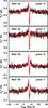 |
Fig. A.1 Comparison of the WBS (red) and HRS (black) spectra obtained at 894 GHz with Herschel/HIFI towards IRAS 4A and IRAS 4B for the H and V polarizations. |
Appendix B: SiO and HDO: The same origin?
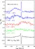 |
Fig. B.1 Comparison of the HDO 11,1–00,0 transition (black) observed towards IRAS 4A and the SiO ν= 0 J = 2–1 line observed towards IRAS 4A (green), a position in the red part of the outflow (red, position (+ 0″, + 20″) with respect to IRAS4A) and two positions in the blue part of the outflow (blue, upper spectra: position (− 12″, − 16″), lower spectra: position (− 12″, − 4″)). The narrow emission line of SiO appears at the same velocity as the thin absorbing layer of HDO. |
The present observations towards the IRAS 4 region reveal an interesting similarity between the deep absorbing components of HDO and the narrow SiO emission line detected by Lefloch et al. (1998). The latter shows a velocity and a linewidth consistent with the HDO absorbing component (see Fig. B.1), which could suggest a common origin. The narrow SiO emission is quite extended (~200″, see Fig. 2 in Lefloch et al. 1998), as we have also inferred for the HDO absorbing layer (see Sect. 3.3). Variations of the narrow SiO line intensity are observed along the NGC 1333 complex, with particularly bright lines around the blue lobe and non-detections towards the source and the red lobe. From LVG (Large Velocity Gradient) modeling of the bright SiO narrow components in the blue lobe, Lefloch et al. (1998) estimated the SiO column density of (1 − 5) × 1012 cm-2 and the H2 density at about (1 − 5) × 105 cm-3, assuming a gas temperature of 33 K equal to that of the dust. For the same SiO column density and a lower H2 density (~104 cm-3), the intensity of the SiO ν= 0 J = 2–1 line is only 0.07 K, in agreement with the non-detection by Lefloch et al. of narrow SiO emission towards our HDO spectra positions (≲0.27 K for both the source position and the red lobe). To reproduce the HDO absorbing components with the RATRAN modeling, it is also necessary to restrain the H2 density at a lower value (<105 cm-3; see Sect. 3.3). A layer of constant column density but subject to density variations (n(H2) < 105 cm-3 towards the sources and the red lobe and n(H2) ~ (1 − 5) × 105 cm-3 towards the blue lobe) could then explain both the deep HDO absorptions and the lack of detectable SiO narrow emission towards the sources and the red lobe as well as the bright SiO narrow emission towards the blue lobe. Alternatively, a layer of uniform low density ~104 cm-3, but with gas temperature locally increasing to ~80–100 K towards the blue lobe, would explain why SiO is only detected in this region. In these cases, the HDO absorptions should be shallower towards the blue part of the outflow. Unfortunately, no HDO observation is available at this position to confirm it. Assuming that the HDO column density of the absorbing layer does not vary significantly between IRAS 4A and the blue outflow lobe, the SiO/HDO abundance ratio in this layer would be ~0.07–0.35. The beam sizes of the HDO 11,1–00,0 line at 894 GHz and the SiO ν= 0 J = 2–1 transition mapped by Lefloch et al. (1998) with the IRAM-30 m telescope are similar.
Another argument suggesting that the narrow HDO and SiO components may trace the same layer is that, in dense and dark clouds, both of these species are believed to be mostly trapped in dust grains and their associated icy mantles. Hence, the same mechanism could release SiO (or other Si components) at the same time as HDO and H2O into the gas phase. We discuss below two mechanisms able to release these molecules into the gas phase: photodesorption and shocks. Another mechanism proposed by Yıldız et al. (2012) to explain detections of narrow 13CO emission lines within the outflow lobes of IRAS 4A is UV-heating by the central source. The narrow SiO emission in NGC 1333 has a more extended spatial distribution, which instead tends to peak outside of the outflow cavities (see Fig. 1 in Lefloch et al. 1998), which appears to rule out this interpretation here.
Appendix B.1: Photodesorption
It was suggested that narrow SiO emission at the systemic velocity could be produced by photodesorption mechanisms in photodissociation regions (PDR) such as the Orion bar (Walmsley et al. 1999; Schilke et al. 2001). Indeed, the strength of Si+ in irradiated regions suggests that up to ~10% of the elemental silicon is not locked in silicate grain cores, but in less refractory material that gets efficiently desorbed at low AV (Haas et al. 1986). We note that a similar fraction of silicon (~5%) with respect to the cosmic abundance (~3 × 10⁻⁵) is measured in the gas-phase of diffuse clouds (e.g., Morton 1975; Sofia et al. 1994; Miller et al. 2007). Gusdorf et al. (2008b) also estimated that, to account for the observed SiO line intensities in the blue lobe of L1157, about ~10% of the silicon assumed in the form of SiO has to be locked in the grain mantles.
Photodesorption could then release SiO in the gas phase simultaneously with water and HDO. Alternatively, the material could be trapped in grain mantles in the form of atomic Si; the Si would then be desorbed and react with O2 or OH to form SiO according to the following reactions (Walmsley et al. 1999):  The balance between photodesorption and photodissociation predicts an SiO-enriched layer located at some depth behind the photodissociation front, which can easily explain the SiO column density observed towards the Orion Bar of a few 1012 cm-2 (Walmsley et al. 1999; Schilke et al. 2001). Although O2 is actually less abundant than assumed in these early models, a tentative detection of O2 was recently reported towards IRAS 4A at a velocity (~8.0 km s-1) close to our HDO absorptions (~7.6 km s-1), and suggested to be produced by photodesorption mechanisms (Yıldız et al. 2013). Photodissociation of H2O would also produce ample OH to react with Si and form SiO by the second reaction above.
Photodesorption of grain mantles thus appears as a possible explanation for the narrow HDO and SiO components at the systemic velocity towards the IRAS 4A region. Photodissociation region models appropriate for the surface of the NGC 1333 cloud, i.e., with lower UV radiation field (χ ~ 1) than the Orion bar (χ ~ 104–105), could verify if this mechanism also reproduces the observed SiO/HDO ratio.
Appendix B.2: Shocks
Shocks are another non-thermal mechanism able to remove both silicon and water from dust grains. Contrary to CO that traces all of the entrained material in molecular flows, broad SiO emission is mostly detected in the youngest outflows from Class 0 protostars (Gibb et al. 2004). This is not surprising, as SiO requires a higher density than CO for excitation and especially shocks fast enough (≥10 − 25 km s-1) to efficiently sputter SiO and Si from the mantles and grain cores in which they would otherwise remain locked (Schilke et al. 1997; Caselli et al. 1997; Gusdorf et al. 2008a,b; Guillet et al. 2009). Sputtering processes also efficiently release water ice from grain mantles, as illustrated, for example, by the similarity of the SiO and H2O high-velocity wings in the L1157 outflow (Lefloch et al. 2010), and the broad wings in the HDO profile towards IRAS 4A (see Fig. B.1). The IRAS 4A outflow wings have a total SiO column density of a few 1013 cm-2 and an abundance relative to CO ~ 3 × 10⁻⁴ (Lefloch et al. 1998), typical of young outflows (Tafalla et al. 2010). The narrow SiO component towards IRAS 4A has a column density that is 10 times smaller than the column density in the broad SiO component, and an abundance relative to CO that is 100 times lower, when compared to the total C18O at systemic velocity (Lefloch et al. 1998). Hence, the presence of the narrow SiO and HDO components could be explained in this context if about 10% of the SiO (and HDO) released in outflow shocks suffered strong deceleration and chemical dilution (by a typical factor of 10–100) due to turbulent mixing with static ambient gas (Lefloch et al. 1998; Codella et al. 1999). The surface dilution induced by the mixing process would be compensated by the contribution of neighboring outflows, which cover a large fraction of the surface area in NGC 1333. The SiO/HDO ratio is estimated in the outflows at 0.25–1.5 (using N(SiO) = 1–3 × 1013 cm-2 from Lefloch et al. 1998 and N(HDO) = 2–4 × 1013 cm-2 from Sect. 3.4). This could be consistent with that estimated for the narrow layer (0.07–0.35), raising the possibility that shocked gas could contribute to this extended SiO/HDO layer. The SiO and HDO molecules will then re-deplete onto grain mantles on timescales depending on the volume densities (~104 years for densities about 105 cm-3 and ~105 years for densities about 104 cm-3). Numerical simulations would be helpful to compare the predicted SiO/HDO ratio with the observations as well as to verify that sufficient deceleration can indeed be reached before SiO and HDO are readsorbed onto the grains to produce narrow SiO and HDO features close to systemic velocity.
Interactions of magnetic and/or radiative shock precursors with the ambient pre-shocked clumpy medium were also mentioned as a potential mechanism leading to the emission of narrow SiO lines (Jiménez-Serra et al. 2004, 2010, 2011). This interpretation was supported by the higher degree of excitation of the ion fluid compared to the neutral fluid towards the protostar L1448-mm. Roberts et al. (2012) showed, however, that the higher excitation of H13CO+ in the narrow component is not a conclusive indication of a precursor (it could simply be due to protostellar heating). This interpretation then relies entirely on the fact that the narrow SiO emission is compact and spatially confined to the regions around protostars. In the NGC 1333 complex, the narrow SiO component is spatially extended over the whole region (Lefloch et al. 1998). Therefore, the shock precursor interpretation would not hold here.
The HDO/H2O ratio refers to twice the water D/H abundance ratio.
We call warm HDO/H2O ratios the HDO/H2O ratios measured in the warm gas of the protostellar envelope (T ≥ 100 K). The cold HDO/H2O ratios refer then to the measure in the cold gas of the outer envelope (T < 100 K).
CASSIS (http://cassis.irap.omp.eu) has been developed by IRAP-UPS/CNRS.
The HDO abundances quoted in the paper correspond to the N(HDO)/N(H2) ratio.
Acknowledgments
The authors thank D. C. Lis for his comments on the manuscript. HIFI has been designed and built by a consortium of institutes and university departments from across Europe, Canada, and the United States under the leadership of SRON Netherlands Institute for Space Research, Groningen, The Netherlands, and with major contributions from Germany, France, and the US. Consortium members are: Canada: CSA, U. Waterloo; France: IRAP (formerly CESR), LAB, LERMA, IRAM; Germany: KOSMA, MPIfR, MPS; Ireland, NUI Maynooth; Italy: ASI, IFSI-INAF, Osservatorio Astrofisico di Arcetri-INAF; Netherlands: SRON, TUD; Poland: CAMK, CBK; Spain: Observatorio Astronómico Nacional (IGN), Centro de Astrobiología (CSIC-INTA). Sweden: Chalmers University of Technology – MC2, RSS & GARD; Onsala Space Observatory; Swedish National Space Board, Stockholm University – Stockholm Observatory; Switzerland: ETH Zurich, FHNW; USA: Caltech, JPL, NHSC.
References
- André, P., Ward-Thompson, D., & Barsony, M. 1993, ApJ, 406, 122 [NASA ADS] [CrossRef] [Google Scholar]
- Belloche, A., Hennebelle, P., & André, P. 2006, A&A, 453, 145 [NASA ADS] [CrossRef] [EDP Sciences] [Google Scholar]
- Bergin, E. A., Phillips, T. G., Comito, C., et al. 2010, A&A, 521, L20 [NASA ADS] [CrossRef] [EDP Sciences] [Google Scholar]
- Blake, G. A., Sandell, G., van Dishoeck, E. F., et al. 1995, ApJ, 441, 689 [Google Scholar]
- Bockelée-Morvan, D., Gautier, D., Lis, D. C., et al. 1998, Icarus, 133, 147 [NASA ADS] [CrossRef] [Google Scholar]
- Bontemps, S., Andre, P., Terebey, S., & Cabrit, S. 1996, A&A, 311, 858 [NASA ADS] [Google Scholar]
- Bottinelli, S., Ceccarelli, C., Lefloch, B., et al. 2004, ApJ, 615, 354 [NASA ADS] [CrossRef] [Google Scholar]
- Bottinelli, S., Ceccarelli, C., Williams, J. P., & Lefloch, B. 2007, A&A, 463, 601 [NASA ADS] [CrossRef] [EDP Sciences] [Google Scholar]
- Campins, H., & Lauretta, D. S. 2004, in AAS/Division for Planetary Sciences Meeting Abstracts #36, BAAS, 36, 1118 [NASA ADS] [Google Scholar]
- Caselli, P., Hartquist, T. W., & Havnes, O. 1997, A&A, 322, 296 [NASA ADS] [Google Scholar]
- Caselli, P., Keto, E., Bergin, E. A., et al. 2012, ApJ, 759, L37 [Google Scholar]
- Cazaux, S., Cobut, V., Marseille, M., Spaans, M., & Caselli, P. 2010, A&A, 522, A74 [NASA ADS] [CrossRef] [EDP Sciences] [Google Scholar]
- Cazaux, S., Caselli, P., & Spaans, M. 2011, ApJ, 741, L34 [NASA ADS] [CrossRef] [Google Scholar]
- Ceccarelli, C., Hollenbach, D. J., & Tielens, A. G. G. M. 1996, ApJ, 471, 400 [Google Scholar]
- Ceccarelli, C., Castets, A., Caux, E., et al. 2000, A&A, 355, 1129 [NASA ADS] [Google Scholar]
- Ceccarelli, C., Bacmann, A., Boogert, A., et al. 2010, A&A, 521, L22 [NASA ADS] [CrossRef] [EDP Sciences] [Google Scholar]
- Choi, M. 2001, ApJ, 553, 219 [NASA ADS] [CrossRef] [Google Scholar]
- Choi, M. 2005, ApJ, 630, 976 [NASA ADS] [CrossRef] [Google Scholar]
- Choi, M., Kamazaki, T., Tatematsu, K., & Panis, J.-F. 2004, ApJ, 617, 1157 [NASA ADS] [CrossRef] [Google Scholar]
- Codella, C., Bachiller, R., & Reipurth, B. 1999, A&A, 343, 585 [NASA ADS] [Google Scholar]
- Codella, C., Ceccarelli, C., Nisini, B., et al. 2010, A&A, 522, L1 [NASA ADS] [CrossRef] [EDP Sciences] [Google Scholar]
- Coutens, A., Vastel, C., Caux, E., et al. 2012, A&A, 539, A132 [NASA ADS] [CrossRef] [EDP Sciences] [Google Scholar]
- Coutens, A., Vastel, C., Cazaux, S., et al. 2013, A&A, 553, A75 [NASA ADS] [CrossRef] [EDP Sciences] [Google Scholar]
- Crimier, N., Ceccarelli, C., Maret, S., et al. 2010, A&A, 519, A65 [NASA ADS] [CrossRef] [EDP Sciences] [Google Scholar]
- Curtis, E. I., Richer, J. S., & Buckle, J. V. 2010, MNRAS, 401, 455 [NASA ADS] [CrossRef] [Google Scholar]
- Dalgarno, A. 1980, in Interstellar Molecules, ed. B. H. Andrew, IAU Symp., 87, 273 [NASA ADS] [Google Scholar]
- Dartois, E., Thi, W.-F., Geballe, T. R., et al. 2003, A&A, 399, 1009 [NASA ADS] [CrossRef] [EDP Sciences] [Google Scholar]
- de Graauw, T., Helmich, F. P., Phillips, T. G., et al. 2010, A&A, 518, L6 [NASA ADS] [CrossRef] [EDP Sciences] [Google Scholar]
- Di Francesco, J., Myers, P. C., Wilner, D. J., Ohashi, N., & Mardones, D. 2001, ApJ, 562, 770 [NASA ADS] [CrossRef] [Google Scholar]
- Drake, M. J., & Campins, H. 2006, in Asteroids, Comets, Meteors, eds. L. Daniela, M. Sylvio Ferraz, & F. J. Angel, IAU Symp., 229, 381 [Google Scholar]
- Dulieu, F., Amiaud, L., Congiu, E., et al. 2010, A&A, 512, A30 [NASA ADS] [CrossRef] [EDP Sciences] [Google Scholar]
- Evans,II, N. J., Dunham, M. M., Jørgensen, J. K., et al. 2009, ApJS, 181, 321 [NASA ADS] [CrossRef] [Google Scholar]
- Faure, A., Wiesenfeld, L., Scribano, Y., & Ceccarelli, C. 2011, MNRAS, 2015 [Google Scholar]
- Flower, D. R., & Pineau des Forêts, G. 1994, MNRAS, 268, 724 [NASA ADS] [CrossRef] [Google Scholar]
- Fraser, H. J., Collings, M. P., McCoustra, M. R. S., & Williams, D. A. 2001, MNRAS, 327, 1165 [NASA ADS] [CrossRef] [Google Scholar]
- Froebrich, D. 2005, ApJS, 156, 169 [NASA ADS] [CrossRef] [Google Scholar]
- Geiss, J., & Gloeckler, G. 1998, Space Sci. Rev., 84, 239 [NASA ADS] [CrossRef] [Google Scholar]
- Genda, H., & Ikoma, M. 2008, Icarus, 194, 42 [NASA ADS] [CrossRef] [Google Scholar]
- Gibb, A. G., Richer, J. S., Chandler, C. J., & Davis, C. J. 2004, ApJ, 603, 198 [NASA ADS] [CrossRef] [Google Scholar]
- Guillet, V., Jones, A. P., & Pineau DesForêts, G. 2009, A&A, 497, 145 [Google Scholar]
- Gusdorf, A., Cabrit, S., Flower, D. R., & Pineau DesForêts, G. 2008a, A&A, 482, 809 [Google Scholar]
- Gusdorf, A., Pineau DesForêts, G., Cabrit, S., & Flower, D. R. 2008b, A&A, 490, 695 [NASA ADS] [CrossRef] [EDP Sciences] [Google Scholar]
- Haas, M. R., Hollenbach, D. J., & Erickson, E. F. 1986, ApJ, 301, L57 [NASA ADS] [CrossRef] [Google Scholar]
- Hartogh, P., Lis, D. C., Bockelée-Morvan, D., et al. 2011, Nature, 478, 218 [NASA ADS] [CrossRef] [PubMed] [Google Scholar]
- Hirota, T., Bushimata, T., Choi, Y. K., et al. 2008, PASJ, 60, 37 [NASA ADS] [CrossRef] [Google Scholar]
- Hogerheijde, M. R., & van der Tak, F. F. S. 2000, A&A, 362, 697 [NASA ADS] [Google Scholar]
- Hollenbach, D., & McKee, C. F. 1979, ApJS, 41, 555 [NASA ADS] [CrossRef] [Google Scholar]
- Hollenbach, D., Kaufman, M. J., Bergin, E. A., & Melnick, G. J. 2009, ApJ, 690, 1497 [CrossRef] [Google Scholar]
- Ikoma, M., & Genda, H. 2006, LPI Contributions, 1335, 50 [NASA ADS] [Google Scholar]
- Ioppolo, S., Cuppen, H. M., Romanzin, C., van Dishoeck, E. F., & Linnartz, H. 2008, ApJ, 686, 1474 [NASA ADS] [CrossRef] [Google Scholar]
- Jensen, M. J., Bilodeau, R. C., Safvan, C. P., et al. 2000, ApJ, 543, 764 [NASA ADS] [CrossRef] [Google Scholar]
- Jiménez-Serra, I., Martín-Pintado, J., Rodríguez-Franco, A., & Marcelino, N. 2004, ApJ, 603, L49 [NASA ADS] [CrossRef] [Google Scholar]
- Jiménez-Serra, I., Caselli, P., Tan, J. C., et al. 2010, MNRAS, 406, 187 [NASA ADS] [CrossRef] [Google Scholar]
- Jiménez-Serra, I., Martín-Pintado, J., Winters, J.-M., Rodríguez-Franco, A., & Caselli, P. 2011, ApJ, 739, 80 [NASA ADS] [CrossRef] [Google Scholar]
- Jørgensen, J. K., & van Dishoeck, E. F. 2010a, ApJ, 725, L172 [NASA ADS] [CrossRef] [Google Scholar]
- Jørgensen, J. K., & van Dishoeck, E. F. 2010b, ApJ, 710, L72 [NASA ADS] [CrossRef] [Google Scholar]
- Jørgensen, J. K., Schöier, F. L., & van Dishoeck, E. F. 2002, A&A, 389, 908 [NASA ADS] [CrossRef] [EDP Sciences] [Google Scholar]
- Jørgensen, J. K., Hogerheijde, M. R., van Dishoeck, E. F., Blake, G. A., & Schöier, F. L. 2004, A&A, 413, 993 [NASA ADS] [CrossRef] [EDP Sciences] [Google Scholar]
- Jørgensen, J. K., Bourke, T. L., Myers, P. C., et al. 2007, ApJ, 659, 479 [NASA ADS] [CrossRef] [Google Scholar]
- Jørgensen, J. K., van Dishoeck, E. F., Visser, R., et al. 2009, A&A, 507, 861 [NASA ADS] [CrossRef] [EDP Sciences] [Google Scholar]
- Karska, A., Herczeg, G. J., van Dishoeck, E. F., et al. 2013, A&A, 552, A141 [NASA ADS] [CrossRef] [EDP Sciences] [Google Scholar]
- Kristensen, L. E., Visser, R., van Dishoeck, E. F., et al. 2010, A&A, 521, L30 [NASA ADS] [CrossRef] [EDP Sciences] [Google Scholar]
- Kristensen, L. E., van Dishoeck, E. F., Bergin, E. A., et al. 2012, A&A, 542, A8 [NASA ADS] [CrossRef] [EDP Sciences] [Google Scholar]
- Langer, W. D., Castets, A., & Lefloch, B. 1996, ApJ, 471, L111 [NASA ADS] [CrossRef] [Google Scholar]
- Lay, O. P., Carlstrom, J. E., & Hills, R. E. 1995, ApJ, 452, L73 [NASA ADS] [CrossRef] [Google Scholar]
- Lecuyer, C., Gillet, P., & Robert, F. 1998, Chem. Geol., 145, 249 [NASA ADS] [CrossRef] [Google Scholar]
- Lefloch, B., Castets, A., Cernicharo, J., & Loinard, L. 1998, ApJ, 504, L109 [NASA ADS] [CrossRef] [Google Scholar]
- Lefloch, B., Cabrit, S., Codella, C., et al. 2010, A&A, 518, L113 [NASA ADS] [CrossRef] [EDP Sciences] [Google Scholar]
- Levenberg, K. 1944, Quart. Appl. Math., 2, 164 [Google Scholar]
- Liu, F., Parise, B., Kristensen, L., et al. 2011, A&A, 527, A19 [NASA ADS] [CrossRef] [EDP Sciences] [Google Scholar]
- Lunine, J. I., Chambers, J., Morbidelli, A., & Leshin, L. A. 2003, Icarus, 165, 1 [NASA ADS] [CrossRef] [Google Scholar]
- Maret, S., Ceccarelli, C., Caux, E., Tielens, A. G. G. M., & Castets, A. 2002, A&A, 395, 573 [NASA ADS] [CrossRef] [EDP Sciences] [Google Scholar]
- Marquardt, D. 1963, SIAM J. Appl. Math, 11, 431 [Google Scholar]
- Meier, R., Owen, T. C., Matthews, H. E., et al. 1998, Science, 279, 842 [NASA ADS] [CrossRef] [PubMed] [Google Scholar]
- Miller, A., Lauroesch, J. T., Sofia, U. J., Cartledge, S. I. B., & Meyer, D. M. 2007, ApJ, 659, 441 [NASA ADS] [CrossRef] [Google Scholar]
- Miyauchi, N., Hidaka, H., Chigai, T., et al. 2008, Chem. Phys. Lett., 456, 27 [NASA ADS] [CrossRef] [Google Scholar]
- Morbidelli, A., Chambers, J., Lunine, J. I., et al. 2000, Meteoritics and Planetary Science, 35, 1309 [Google Scholar]
- Morton, D. C. 1975, ApJ, 197, 85 [NASA ADS] [CrossRef] [Google Scholar]
- Mottram, J. C., van Dishoeck, E. F., Schmalzl, M., et al. 2013, A&A, 558, A126 [NASA ADS] [CrossRef] [EDP Sciences] [Google Scholar]
- Myers, P. C., & Ladd, E. F. 1993, ApJ, 413, L47 [NASA ADS] [CrossRef] [Google Scholar]
- Niemann, H. B., Atreya, S. K., Carignan, G. R., et al. 1996, Science, 272, 846 [NASA ADS] [CrossRef] [PubMed] [Google Scholar]
- Öberg, K. I., Linnartz, H., Visser, R., & van Dishoeck, E. F. 2009, ApJ, 693, 1209 [NASA ADS] [CrossRef] [Google Scholar]
- O’Brien, D. P., Morbidelli, A., & Levison, H. F. 2006, in 37th Annual Lunar and Planetary Science Conference, eds. S. Mackwell, & E. Stansbery, Lunar and Planetary Inst. Technical Report, 37, 2347 [Google Scholar]
- Ossenkopf, V., & Henning, T. 1994, A&A, 291, 943 [NASA ADS] [Google Scholar]
- Ott, S. 2010, in Astronomical Data Analysis Software and Systems XIX, ASP Conf. Ser., 434, 139 [NASA ADS] [Google Scholar]
- Parise, B., Simon, T., Caux, E., et al. 2003, A&A, 410, 897 [NASA ADS] [CrossRef] [EDP Sciences] [Google Scholar]
- Parise, B., Caux, E., Castets, A., et al. 2005, A&A, 431, 547 [NASA ADS] [CrossRef] [EDP Sciences] [Google Scholar]
- Persson, M. V., Jørgensen, J. K., & van Dishoeck, E. F. 2012, A&A, 541, A39 [NASA ADS] [CrossRef] [EDP Sciences] [Google Scholar]
- Persson, M. V., Jørgensen, J. K., & van Dishoeck, E. F. 2013, A&A, 549, L3 [NASA ADS] [CrossRef] [EDP Sciences] [Google Scholar]
- Phillips, T. G., & Vastel, C. 2003, in SFChem 2002: Chemistry as a Diagnostic of Star Formation, eds. C. L. Curry, & M. Fich, 3 [Google Scholar]
- Pickett, H. M., Poynter, R. L., Cohen, E. A., et al. 1998, J. Quant. Spectr. Rad. Transf., 60, 883 [NASA ADS] [CrossRef] [Google Scholar]
- Pilbratt, G. L., Riedinger, J. R., Passvogel, T., et al. 2010, A&A, 518, L1 [CrossRef] [EDP Sciences] [Google Scholar]
- Pineda, J. E., Maury, A. J., Fuller, G. A., et al. 2012, A&A, 544, L7 [NASA ADS] [CrossRef] [EDP Sciences] [Google Scholar]
- Raymond, S. N., Quinn, T., & Lunine, J. I. 2004, Icarus, 168, 1 [NASA ADS] [CrossRef] [MathSciNet] [Google Scholar]
- Raymond, S. N., Quinn, T., & Lunine, J. I. 2006, Icarus, 183, 265 [NASA ADS] [CrossRef] [Google Scholar]
- Raymond, S. N., O’Brien, D. P., Morbidelli, A., & Kaib, N. A. 2009, Icarus, 203, 644 [NASA ADS] [CrossRef] [Google Scholar]
- Roberts, H., Herbst, E., & Millar, T. J. 2004, A&A, 424, 905 [NASA ADS] [CrossRef] [EDP Sciences] [Google Scholar]
- Roberts, J. F., Jiménez-Serra, I., Gusdorf, A., & Martín-Pintado, J. 2012, A&A, 544, A150 [NASA ADS] [CrossRef] [EDP Sciences] [Google Scholar]
- Roelfsema, P. R., Helmich, F. P., Teyssier, D., et al. 2012, A&A, 537, A17 [NASA ADS] [CrossRef] [EDP Sciences] [Google Scholar]
- Sakai, N., Sakai, T., & Yamamoto, S. 2006, PASJ, 58, L15 [NASA ADS] [Google Scholar]
- Schilke, P., Walmsley, C. M., Pineau des Forêts, G., & Flower, D. R. 1997, A&A, 321, 293 [NASA ADS] [Google Scholar]
- Schilke, P., Pineau des Forêts, G., Walmsley, C. M., & Martín-Pintado, J. 2001, A&A, 372, 291 [NASA ADS] [CrossRef] [EDP Sciences] [Google Scholar]
- Sofia, U. J., Cardelli, J. A., & Savage, B. D. 1994, ApJ, 430, 650 [NASA ADS] [CrossRef] [Google Scholar]
- Stimpfl, M., Lauretta, D. S., & Drake, M. J. 2004, Meteoritics and Planetary Science Supplement, 39, 5218 [NASA ADS] [Google Scholar]
- Tafalla, M., Santiago-García, J., Hacar, A., & Bachiller, R. 2010, A&A, 522, A91 [NASA ADS] [CrossRef] [EDP Sciences] [Google Scholar]
- Taquet, V., López-Sepulcre, A., Ceccarelli, C., et al. 2013a, ApJ, 768, L29 [NASA ADS] [CrossRef] [Google Scholar]
- Taquet, V., Peters, P. S., Kahane, C., et al. 2013b, A&A, 550, A127 [NASA ADS] [CrossRef] [EDP Sciences] [Google Scholar]
- Thi, W.-F., Woitke, P., & Kamp, I. 2010, MNRAS, 407, 232 [NASA ADS] [CrossRef] [Google Scholar]
- Tielens, A. G. G. M., & Hagen, W. 1982, A&A, 114, 245 [NASA ADS] [Google Scholar]
- van der Tak, F. F. S., Black, J. H., Schöier, F. L., Jansen, D. J., & van Dishoeck, E. F. 2007, A&A, 468, 627 [NASA ADS] [CrossRef] [EDP Sciences] [Google Scholar]
- van Dishoeck, E. F., Kristensen, L. E., Benz, A. O., et al. 2011, PASP, 123, 138 [NASA ADS] [CrossRef] [Google Scholar]
- Vastel, C., Ceccarelli, C., Caux, E., et al. 2010, A&A, 521, L31 [NASA ADS] [CrossRef] [EDP Sciences] [Google Scholar]
- Villanueva, G. L., Mumma, M. J., Bonev, B. P., et al. 2009, ApJ, 690, L5 [NASA ADS] [CrossRef] [Google Scholar]
- Visser, R., Jørgensen, J. K., Kristensen, L. E., van Dishoeck, E. F., & Bergin, E. A. 2013, ApJ, 769, 19 [NASA ADS] [CrossRef] [Google Scholar]
- Vuong, M. H., Montmerle, T., Grosso, N., et al. 2003, A&A, 408, 581 [NASA ADS] [CrossRef] [EDP Sciences] [Google Scholar]
- Wagner, A. F., & Graff, M. M. 1987, ApJ, 317, 423 [NASA ADS] [CrossRef] [Google Scholar]
- Walmsley, C. M., Pineau des Forêts, G., & Flower, D. R. 1999, A&A, 342, 542 [NASA ADS] [Google Scholar]
- Walsh, A. J., Bourke, T. L., & Myers, P. C. 2006, ApJ, 637, 860 [NASA ADS] [CrossRef] [Google Scholar]
- Wiesenfeld, L., Scribano, Y., & Faure, A. 2011, Physical Chemistry Chemical Physics (Incorporating Faraday Transactions), 13, 8230 [NASA ADS] [CrossRef] [Google Scholar]
- Yıldız, U. A., Kristensen, L. E., van Dishoeck, E. F., et al. 2012, A&A, 542, A86 [NASA ADS] [CrossRef] [EDP Sciences] [Google Scholar]
- Yıldız, U. A., Acharyya, K., Goldsmith, P. F., et al. 2013, A&A, 558, A58 [NASA ADS] [CrossRef] [EDP Sciences] [Google Scholar]
All Tables
HDO abundances with respect to H2 determined in several low-mass star-forming regions.
All Figures
|
Fig. 1 Energy level diagram of the HDO lines. In red, IRAM-30 m observations; in magenta, JCMT/APEX observation; in blue, HIFI observations. The frequencies are written in GHz. |
| In the text | |
|
Fig. 2 Upper-left panel: HIFI observations of the fundamental line at 894 GHz towards the protostar IRAS 4A (black) and an outflow position (red, discussed in Sect. 3.3). The spectrum at the outflow position has been shifted vertically by 0.178 K. Upper-right panel: JCMT observations of the fundamental line at 465 GHz towards IRAS 4A. Lower-left panel: HIFI observations of the fundamental line at 894 GHz towards the protostar IRAS 4B. Lower-right panel: APEX observations of the fundamental line at 465 GHz towards IRAS 4B. The continuum refers to SSB data for each panel. |
| In the text | |
|
Fig. 3 Decomposition of the 11,1–00,0 fundamental transitions observed towards IRAS 4A and IRAS 4B with HIFI in three Gaussians: a broad emission component (red), a narrower emission component (green), and a narrow absorption component (blue). The parameters of the Gaussian fits are given in Table 2. |
| In the text | |
|
Fig. 4 Comparison of the modeling of the HDO 11,1–00,0 and 10,1–00,0 fundamental transitions observed towards IRAS 4A with an added absorbing layer (in green) and without this layer (in red). The HDO column density in the absorbing layer is about 1.4 × 1013 cm-3. The broad outflow component seen in the observations was subtracted. The continuum refers to SSB data. |
| In the text | |
|
Fig. 5 In black: HDO lines observed towards IRAS 4A with HIFI, IRAM, and JCMT. The broad outflow component seen in the observations was subtracted. The continuum seen in the observations of the 894 GHz and 465 GHz lines refers to SSB data. In red: best-fit model obtained when adding an absorbing layer with an HDO column density of ~1.4 × 1013 cm-2 to the structure. The best-fit inner abundance is 7.5 × 10⁻⁹ and the best-fit outer abundance is 1.2 × 10⁻¹¹. |
| In the text | |
|
Fig. 6 χ2 contours at 1σ, 2σ, and 3σ obtained for IRAS 4A when adding an absorbing layer with an HDO column density of 1.4 × 1013 cm-2 to the structure. The best-fit model is represented by the symbol “+”. The mass is equal to 0.5 M⊙. |
| In the text | |
|
Fig. 7 In black: HDO lines observed towards IRAS 4B with HIFI, IRAM, and APEX. The broad outflow component seen in the observations was subtracted. The continuum seen in the observations of the 894 GHz and 465 GHz lines refers to SSB data. In red: best-fit model obtained when adding the absorbing layer used to model the IRAS 4A lines (N(HDO) ~ 1.4 × 1013 cm-2). The best-fit inner abundance is 1 × 10⁻⁸ and the best-fit outer abundance is 1.2 × 10⁻¹⁰. |
| In the text | |
|
Fig. 8 χ2 contours at 1σ, 2σ, and 3σ obtained for IRAS 4B when adding the absorbing layer used to model the IRAS 4A lines. The best-fit model is represented by the symbol “+”. The mass is equal to 0.1 M⊙. |
| In the text | |
|
Fig. 9 Different scenarios for the position of the absorbing layer with respect to the protostar and the outflows and influence on the absorbing line depth. In case a), the absorbing layer is less extended than the outflows. The continuum that is absorbed is only due to the protostar. The broad component is superposed. In case b), the absorbing layer is more extended than the outflows. The continuum that is absorbed is due both to the protostar and the outflows. |
| In the text | |
|
Fig. 10 Comparison of the line profiles of the CO 6–5 transition (in red), the HDO 11,1–00,0 transition (in black, intensities multiplied by 150), and the H2O 11,1–00,0 transition (in green, intensities multiplied by 15) towards IRAS 4A. |
| In the text | |
|
Fig. 11 Upper panels: comparison of the inner (red) and outer (black) HDO abundances estimated in the low-mass protostars IRAS 16293-2422, NGC 1333 IRAS 4A, NGC 1333 IRAS 2A, and L1448-mm (see also Table 3) as a function of a) the ratio between the submillimeter and bolometric luminosities Lsmm/Lbol; b) the bolometric luminosity Lbol; c) the submillimeter luminosity Lsmm; d) the bolometric temperature Tbol; e) the ratio |
| In the text | |
|
Fig. A.1 Comparison of the WBS (red) and HRS (black) spectra obtained at 894 GHz with Herschel/HIFI towards IRAS 4A and IRAS 4B for the H and V polarizations. |
| In the text | |
|
Fig. B.1 Comparison of the HDO 11,1–00,0 transition (black) observed towards IRAS 4A and the SiO ν= 0 J = 2–1 line observed towards IRAS 4A (green), a position in the red part of the outflow (red, position (+ 0″, + 20″) with respect to IRAS4A) and two positions in the blue part of the outflow (blue, upper spectra: position (− 12″, − 16″), lower spectra: position (− 12″, − 4″)). The narrow emission line of SiO appears at the same velocity as the thin absorbing layer of HDO. |
| In the text | |
Current usage metrics show cumulative count of Article Views (full-text article views including HTML views, PDF and ePub downloads, according to the available data) and Abstracts Views on Vision4Press platform.
Data correspond to usage on the plateform after 2015. The current usage metrics is available 48-96 hours after online publication and is updated daily on week days.
Initial download of the metrics may take a while.