| Issue |
A&A
Volume 560, December 2013
|
|
|---|---|---|
| Article Number | A87 | |
| Number of page(s) | 13 | |
| Section | Astrophysical processes | |
| DOI | https://doi.org/10.1051/0004-6361/201322185 | |
| Published online | 11 December 2013 | |
Magnetic field amplification in young galaxies
1
Universität Heidelberg, Zentrum für Astronomie, Institut für Theoretische
Astrophysik, Albert-Ueberle-Strasse
2, 69120
Heidelberg,
Germany
e-mail: This email address is being protected from spambots. You need JavaScript enabled to view it.
2
Georg-August-Universität Göttingen, Institut für
Astrophysik, Friedrich-Hund-Platz
1, 37077
Göttingen,
Germany
Received:
1
July
2013
Accepted:
7
November
2013
Abstract
The Universe at present is highly magnetized, with fields of a few 10-5 G and coherence lengths greater than 10 kpc in typical galaxies like the Milky Way. We propose that the magnetic field was already amplified to these values during the formation and the early evolution of galaxies. Turbulence in young galaxies is driven by accretion, as well as by supernova (SN) explosions of the first generation of stars. The small-scale dynamo can convert the turbulent kinetic energy into magnetic energy and amplify very weak primordial seed fields on short timescales. Amplification takes place in two phases: in the kinematic phase the magnetic field grows exponentially, with the largest growth rate on the smallest nonresistive scale. In the following nonlinear phase the magnetic energy is shifted toward larger scales until the dynamo saturates on the turbulent forcing scale. To describe the amplification of the magnetic field quantitatively, we modeled the microphysics in the interstellar medium (ISM) of young galaxies and determined the growth rate of the small-scale dynamo. We estimated the resulting saturation field strengths and dynamo timescales for two turbulent forcing mechanisms: accretion-driven turbulence and SN-driven turbulence. We compare them to the field strength that is reached when only stellar magnetic fields are distributed by SN explosions. We find that the small-scale dynamo is much more efficient in magnetizing the ISM of young galaxies. In the case of accretion-driven turbulence, a magnetic field strength on the order of 10-6 G is reached after a time of 24−270 Myr, while in SN-driven turbulence the dynamo saturates at field strengths of typically 10-5 G after only 4−15 Myr. This is considerably shorter than the Hubble time. Our work can help for understanding why present-day galaxies are highly magnetized.
Key words: ISM: magnetic fields / galaxies: high-redshift / galaxies: magnetic fields / dynamo / magnetic fields / turbulence
© ESO, 2013
1. Introduction
The present-day Universe is filled with magnetic fields. Observations show that galaxies (Beck et al. 1999; Beck 2011) and stars (Donati & Landstreet 2009; Reiners 2012) are strongly magnetized, and there are also hints of weak magnetic fields in the intergalactic medium (Kim et al. 1989; Kronberg 1994; Neronov et al. 2013). The origin of these strong fields remains an unsolved problem in astrophysics.
Local spiral galaxies typically have turbulent field components of (2−3) × 10-5 G within the arms and bars, while a field of (5−10) × 10-5 G is observed in the central starburst regions. Moreover, these fields appear to be coherent on scales larger than 10 kpc, which is the same order of magnitude as the size of the galaxy. The magnetic energy in the galactic interstellar medium (ISM) is thus approximately in equipartition with the thermal energy and the energy in cosmic rays. The field in the interarm region is usually ordered and has a strength on the order of (1−1.5) × 10-5 G (Beck 2011). Also dwarf irregular galaxies have magnetic fields: however, they appear not to be ordered on large scales and have a lower strength of ≤4 × 10⁻⁶ G (Chyży et al. 2011).
New observations indicate that even highly redshifted galaxies have magnetic field strengths comparable to present-day galaxies (Bernet et al. 2008). For instance, the rotation measure, a quantity that depends on the magnetic field along the line of sight, is constant up to redshifts of roughly 5 (Hammond et al. 2012). An important tool is, moreover, the far-infrared radio correlation, which can be interpreted as a relation between the star formation rate and the synchrotron radiation of cosmic ray electrons in magnetic fields (Sargent et al. 2010; Bourne et al. 2011) and appears to be valid until z ≈ 2 (Murphy 2009). We note, however, that one expects a breakdown at higher redshift as a result of inverse Compton scattering with cosmic microwave background photons (Schleicher & Beck 2013). Observations of the intergalactic medium provide further information on primordial seed fields. Detailed analysis of the CMB temperature bispectrum using data from the Planck satellite gives an upper limit of the magnetic field strength of a few nG on the Mpc scale (Shiraishi et al. 2012). The increasing evidence of magnetic fields in highly redshifted galaxies and the intergalactic medium indicates an early generation of the magnetic fields.
Theoretically, the first seed fields might have already been generated in the very early
Universe during inflation, leading to a field strength of
B0 ≈ 10-34–10-10 G on a scale of 1 Mpc
(Turner & Widrow 1988). Another generation
mechanism are first-order phase transitions. Sigl et al.
(1997) predict a field strength of
B0 ≈ 10-29 G from the electroweak phase transition
and B0 ≈ 10-20 G from the QCD phase transition on a
scale of 10 Mpc. The correlation length of the primordial magnetic seed fields has been
shown to crucially depend on the initial properties of the field, e.g., on the amount of
magnetic helicity (Banerjee & Jedamzik 2004). We
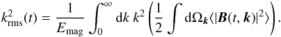
can determine the typical strength of a statistical seed field by writing the magnetic
energy as  . Magnetic fields can be also generated as a
result of the Biermann term in the generalized Ohm’s law, which takes the different behavior
of the electron and ion fluid into account (Biermann
1950; Kulsrud & Zweibel 2008). A typical
field strength resulting from this so-called “Biermann battery” is 10-19 G
(Xu et al. 2008 ). Recently, Schlickeiser (2012) has shown that a turbulent magnetic field can be
generated in plasma fluctuations within an unmagnetized nonrelativistic medium. From this
effect we would expect typical seed fields of a few 10-10 G within the first
galaxies. Although this exceeds the resulting field strengths of other generation mechanisms
it still cannot explain the typical values in local galaxies. Thus, amplification processes
need to take place.
. Magnetic fields can be also generated as a
result of the Biermann term in the generalized Ohm’s law, which takes the different behavior
of the electron and ion fluid into account (Biermann
1950; Kulsrud & Zweibel 2008). A typical
field strength resulting from this so-called “Biermann battery” is 10-19 G
(Xu et al. 2008 ). Recently, Schlickeiser (2012) has shown that a turbulent magnetic field can be
generated in plasma fluctuations within an unmagnetized nonrelativistic medium. From this
effect we would expect typical seed fields of a few 10-10 G within the first
galaxies. Although this exceeds the resulting field strengths of other generation mechanisms
it still cannot explain the typical values in local galaxies. Thus, amplification processes
need to take place.
A very efficient mechanism to amplify weak seed fields is the small-scale or turbulent
dynamo, which converts kinetic energy from turbulence into magnetic energy by randomly
stretching and twisting the field lines. The magnetic energy grows exponentially in the
kinematic phase, while the growth rate is largest on the resistive scale (Kazantsev 1968; Subramanian 1997; Brandenburg & Subramanian
2005). There are two dimensionless parameters, which control the efficiency of this
process (Schober et al. 2012b; Bovino et al. 2013): the hydrodynamic Reynolds number  (1)where V is the turbulent
velocity on the outer scale of the inertial range L and ν
is the viscosity, and the magnetic Reynolds number
(1)where V is the turbulent
velocity on the outer scale of the inertial range L and ν
is the viscosity, and the magnetic Reynolds number  (2)with η being the magnetic
resistivity. The ratio of the Reynolds numbers defines the magnetic Prandtl number
(2)with η being the magnetic
resistivity. The ratio of the Reynolds numbers defines the magnetic Prandtl number
 (3)Furthermore, the dynamo growth rate depends on
the type of the turbulence ranging from incompressible Kolmogorov turbulence (Kolmogorov 1941) to highly compressible Burgers
turbulence (Burgers 1948). Eventually the magnetic
field is strong enough for back reactions to occur on the gas and the nonlinear growth sets
in (Schekochihin et al. 2002). In this phase the
magnetic energy is transported toward larger scales. Now the evolution no longer depends on
the Reynolds and Prandtl numbers, but still on the type of turbulence (Schleicher et al. 2013). The nonlinear phase comes to an end, when the
magnetic field reaches saturation on the turbulent forcing scale L.
(3)Furthermore, the dynamo growth rate depends on
the type of the turbulence ranging from incompressible Kolmogorov turbulence (Kolmogorov 1941) to highly compressible Burgers
turbulence (Burgers 1948). Eventually the magnetic
field is strong enough for back reactions to occur on the gas and the nonlinear growth sets
in (Schekochihin et al. 2002). In this phase the
magnetic energy is transported toward larger scales. Now the evolution no longer depends on
the Reynolds and Prandtl numbers, but still on the type of turbulence (Schleicher et al. 2013). The nonlinear phase comes to an end, when the
magnetic field reaches saturation on the turbulent forcing scale L.
Turbulence is driven efficiently for the first time in the history of the Universe when dark matter halos become massive enough that gas begins to cool efficiently and flows into the potential wells of dark matter halos. This leads to the formation of the first generation of stars and the subsequent build-up of galaxies. The first stars form at redhifts between 20 and 15 within primordial minihalos, which have typical masses of more than 105 solar masses (M⊙) (see e.g., Abel et al. 2002; Bromm & Larson 2004; Clark et al. 2011). In recent publications it was shown, numerically as well as semi-analytically, that during the formation of the first stars, dynamically important magnetic fields can be generated by the small-scale dynamo on short timescales (Sur et al. 2012; Turk et al. 2012; Schober et al. 2012a). According to the theory of hierarchical structure formation the first galaxies, also called protogalaxies, form at redshifts smaller than about 10 in massive dark matter halos with more than 107 M⊙ (Greif et al. 2008; Bromm et al. 2009). In young galaxies accretion as well as the penetration of supernovae (SN) shocks through the gas generate turbulence, which initiates small-scale dynamo action (Beck et al. 2012; Latif et al. 2013).
In this paper, we follow the evolution of the magnetic field in an initially weakly magnetized young galaxy. Because the true dynamical nature of the first galaxies is not well known, we adopt two simplified complementary models: a spherical galaxy as well as a disk-like system, both with constant density and temperature. We model microphysical processes, such as the diffusion of the kinematic and magnetic energy, in order to find the magnetohydrodynamical (MHD) quantities, which determine the growth rate of the small-scale dynamo. Turbulence can be generated by accretion flows into the center of the halo, for which we estimate the typical Reynolds numbers. Then we follow the evolution of the magnetic field strength in the kinematic and the nonlinear phase, until saturation on the driving scale of the turbulence is reached. Stellar feedback, in particular SN explosions, also influences the evolution of the magnetic field. On the one hand supernovae distribute stellar magnetic fields in the ISM (Rees 1987), on the other hand they drive turbulence, which again leads to dynamo action (Balsara et al. 2004). We compare the resulting magnetic field strengths from both mechanisms with the field strength gained by an accretion-driven small-scale dynamo.
The outline of the paper is as follows: in Sect. 2 we describe our model. We determine the values of viscosity and magnetic diffusivity in the ISM and estimate the evolution of SN explosions. Driving mechanisms of turbulence are discussed in general. In the last part of this section we summarize the main points of a mathematical description of magnetic field amplification by the small-scale dynamo. The kinematic phase described by the so-called Kazantsev theory and a model for the nonlinear growth phase are introduced. In Sect. 3 we present our results for the evolution of the magnetic field in the different types of models. First we discuss the generation of turbulence by accretion and the resulting efficiencies of the dynamo, i.e. the saturation magnetic field strength and the time until saturation occurs. Second, we analyze the effect of stellar feedback. We compare the efficiency of distributing stellar magnetic fields by SN with the one of the SN-driven turbulent dynamo. We draw our conclusions in Sect. 4.
2. Modeling physical processes in a protogalaxy
2.1. General aspects
The nature of young galaxies is still an active topic of research (see Bromm & Yoshida 2011, for a review). For our order of magnitude estimate of the magnetic field evolution we use a very simplified model, with the choice of parameters being motivated from numerical simulations (Greif et al. 2008; Bromm et al. 2009; Latif et al. 2013). We are interested in massive protogalactic objects at redshifts of roughly 10.
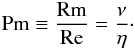
In our model we assume a mean particle density of
 (4)and a temperature of
 (5)The density as well as the temperature are,
as first approximation, constant throughout the whole galaxy. For simplicity we take a gas
into account that only consists of hydrogen, which is at the given values of
n and T mostly ionized.
(5)The density as well as the temperature are,
as first approximation, constant throughout the whole galaxy. For simplicity we take a gas
into account that only consists of hydrogen, which is at the given values of
n and T mostly ionized.
The mean shape of the primordial galaxies differs most probably from the one of present-day galaxies. Due to a significant amount of angular momentum the protogalaxies may form in a spherical way and develop a more disk-like structure at later stages. To account for the unknown typical shape, we model two extreme cases, a spherical and a disk-like galaxy, which have the same gas mass.
Spherical galaxy. In the case of a spherical protogalaxy we assume the radius to be
 (6)As within this radius the density as well as
the temperature are constant we find a total mass of the baryonic gas of
(6)As within this radius the density as well as
the temperature are constant we find a total mass of the baryonic gas of
 (7)
(7)
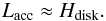
Disk-like galaxy. As our second fiducial model we use a galaxy with disk scale height of
ten percent of the radius, i.e.  (8)With the condition that the gas mass of the
disk needs to be the same as in the spherical case, the disk radius is
(8)With the condition that the gas mass of the
disk needs to be the same as in the spherical case, the disk radius is  (9)
(9)
2.2. Microphysics in the ISM
As the temperature in the primordial ISM is very high, we can assume the gas to be (at
least partially) ionized. We thus need to deal with the full plasma equations, i.e. the
continuity, the momentum and the energy equations for both the ions and the electrons.
Closures of these equations were found by Braginskii
(1965), who used the Chapman-Enskog scheme (Chapman et al. 1953). The closure is based on the assumption that the
macroscopic scale of the plasma is large compared to the mean-free path  (10)or compared to the gyro-radii of the
electrons and the ions
(10)or compared to the gyro-radii of the
electrons and the ions  (11)Here
rc = e2/(kT) is
the distance of closest particle approach with e being the elementary
charge and k the Boltzmann constant. The mass of the species is labeled
ms, where the s stands for electrons (e) or protons (p), and
c is the speed of light. Further, we use here the thermal velocity
(2kT/ms)1/2 and assume that the
temperatures of the ions and electrons are equal
(Te = Tp ≡ T).
In principle, the components of a plasma can have unequal temperatures as during plasma
heating the different fluids are heated differently. However, after a certain time
teq, an equilibrium will be reached. The electron-proton
equilibrium time can be computed by (Spitzer 1956)
(11)Here
rc = e2/(kT) is
the distance of closest particle approach with e being the elementary
charge and k the Boltzmann constant. The mass of the species is labeled
ms, where the s stands for electrons (e) or protons (p), and
c is the speed of light. Further, we use here the thermal velocity
(2kT/ms)1/2 and assume that the
temperatures of the ions and electrons are equal
(Te = Tp ≡ T).
In principle, the components of a plasma can have unequal temperatures as during plasma
heating the different fluids are heated differently. However, after a certain time
teq, an equilibrium will be reached. The electron-proton
equilibrium time can be computed by (Spitzer 1956)
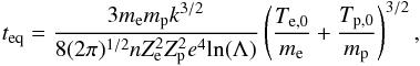 (12)where Zs is the
charge of species s, Ts,0 its initial temperature and the
Coulomb logarithm is defined by
(12)where Zs is the
charge of species s, Ts,0 its initial temperature and the
Coulomb logarithm is defined by 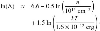 (13)If we assume Te,0
and Tp,0 to be extremely different, e.g.,
Te,0 = 103 Tp,0, the
typical teq for our model is on the order of 440 yr. It will
be shown later that this is way below the typical dynamo timescales, which can be up to
many Myr. Thus, the electron and the proton temperature can be assumed to be equal in our
calculation.
(13)If we assume Te,0
and Tp,0 to be extremely different, e.g.,
Te,0 = 103 Tp,0, the
typical teq for our model is on the order of 440 yr. It will
be shown later that this is way below the typical dynamo timescales, which can be up to
many Myr. Thus, the electron and the proton temperature can be assumed to be equal in our
calculation.
A comparison of the length scales (10) and (11) in our model can be found in Fig. 1. When the gyro-radius becomes smaller than the mean-free path, the magnetic field dominates the dynamics of the plasma, i.e. it becomes “magnetized”. In our model the electron fluid becomes magnetized at a magnetic field strength of roughly 10-12 G, the ion fluid at 10-10 G.
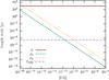 |
Fig. 1 Gyro-radii of electrons and ions ρe and ρp as a function of magnetic field strength compared to the typical macroscopic scale L ≈ 103 pc and the mean-free path ℓmfp. Within our fiducial case for the density and the temperature the electron fluid becomes magnetized at a magnetic field strength of roughly 10-12 G, the ion fluid at 10-10 G. |
2.2.1. Viscosity
In the transition from an unmagnetized to a magnetized state, the plasma becomes anisotropic, i.e. certain physical quantities then depend on their relative orientation to the magnetic field direction.
In the unmagnetized case the kinematic viscosities for electrons and ions obtained from
the Chapman-Enskog closure scheme are (Braginskii
1965) ![Mathematical equation: \begin{eqnarray} \label{nu_parallel_e} \nu_{\parallel,\mathrm{e}} & = & 0.73 \frac{\tau_\mathrm{e} k T}{m_\mathrm{e}} = 1.4\times10^{14}~\mathrm{cm}^2\,\mathrm{s}^{-1} \\[2mm] \label{nu_parallel_p} \nu_{\parallel,\mathrm{p}} & = & 0.96 \frac{\tau_\mathrm{p} k T}{m_\mathrm{p}} = 8.7\times10^{15}~\mathrm{cm}^2\,\mathrm{s}^{-1} \end{eqnarray}](/articles/aa/full_html/2013/12/aa22185-13/aa22185-13-eq60.png) with the collision times for electrons and
ions
with the collision times for electrons and
ions ![Mathematical equation: \begin{eqnarray} \tau_{\mathrm{e}} & = & \frac{6 \sqrt{2} \sqrt{m_\mathrm{e}} (k T)^{3/2}}{16 \pi^{1/2} \mathrm{ln}(\Lambda) e^4 n}\\[2mm] \tau_{\mathrm{p}} & = & \frac{12 \sqrt{m_\mathrm{p}} (k T)^{3/2}}{16 \pi^{1/2} \mathrm{ln}(\Lambda) e^4 n}\cdot \end{eqnarray}](/articles/aa/full_html/2013/12/aa22185-13/aa22185-13-eq61.png) In the presence of a strong magnetic field
the viscosity becomes anisotropic and one has to distinguish between the viscosity along
(parallel to) and the one perpendicular to the magnetic field lines. While the parallel
viscosity stays the same as in the unmagnetized case (e.g., Eqs. (14) and (15)), the viscosity perpendicular to the field is given by (Simon 1955)
In the presence of a strong magnetic field
the viscosity becomes anisotropic and one has to distinguish between the viscosity along
(parallel to) and the one perpendicular to the magnetic field lines. While the parallel
viscosity stays the same as in the unmagnetized case (e.g., Eqs. (14) and (15)), the viscosity perpendicular to the field is given by (Simon 1955) 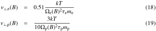 with the gyro-frequencies
 Diffusion perpendicular to the magnetic
field lines is also known as “Bohm diffusion”.
Diffusion perpendicular to the magnetic
field lines is also known as “Bohm diffusion”.
The different viscosities as a function of density are shown in Fig. 2. Note that the perpendicular viscosity only becomes
valid when the plasma is magnetized, i.e. when the gyro-radius becomes smaller than the
mean-free path. According to Fig. 1 this is the
case above a magnetic field strength of 10-11 G for the electrons and
10-9 G for the ions. Thus, the most important part of the viscosity is the
parallel one and we will ignore the perpendicular part, which decreases proportional the
1/B2, from now on. Furthermore, the viscosity of the ions
exceeds the electron viscosity by roughly two orders of magnitude. This is caused by the
fact that the ions carry the largest part of the momentum. In total, the parallel
viscosity of the ions is the crucial quantity and we will refer from now on to
 (22)
(22)
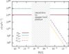 |
Fig. 2 Kinematic viscosity parallel (ν∥) and perpendicular to the magnetic field lines (ν⊥) as a function of magnetic field strength B. We show the results for the electron as well as for the ion fluid. The range between 10-11 G and 10-7 G is not shown, as here the transition from the unmagnetized to a magnetized plasma takes place. |
2.2.2. Magnetic diffusivity
For the parallel conductivity the closure scheme yields (Spitzer 1956)
 (23)and for the conductivity perpendicular to
the magnetic field
(23)and for the conductivity perpendicular to
the magnetic field  (24)The conductivity perpendicular to the
magnetic field lines is, contrary to the case of viscosity, no function of the magnetic
field strength. The difference between the parallel and the perpendicular component of
the conductivity is just approximately a factor of two. Usually,
σ∥ is used to determine the magnetic diffusivity
η of a plasma. We thus find
(24)The conductivity perpendicular to the
magnetic field lines is, contrary to the case of viscosity, no function of the magnetic
field strength. The difference between the parallel and the perpendicular component of
the conductivity is just approximately a factor of two. Usually,
σ∥ is used to determine the magnetic diffusivity
η of a plasma. We thus find  (25)which is also known as “Spitzer
resistivity”.
(25)which is also known as “Spitzer
resistivity”.
2.2.3. Magnetic Prandtl number
With these values of viscosity and resistivity the magnetic Prandtl number (see Eq.
(3)) is
 (26)
(26)
2.3. Turbulence
2.3.1. Generation of turbulent motions by accretion
Structure formation is always associated with accretion. In order to build up the first stars and galaxies, gas flows into the potential wells of dark matter halos, where it gets compressed and cools. The potential energy released during that process in parts gets converted into turbulent kinetic energy (Klessen & Hennebelle 2010). Simulations by Greif et al. (2008) of atomic cooling halos show that two types of accretion occur: in the so-called “hot accretion” mode gas is accreted directly from the intergalactic medium, while in the “cold accretion” mode gas is cooled down and flows into the central regions of the halo at high velocities (Dekel et al. 2009; Nelson et al. 2013).
2.3.2. Generation of turbulent motions by supernova explosions
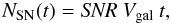
Once stars have formed, their feedback strongly influences the ISM in galaxies in terms of ionizing radiation and at later stages by SN explosions, which are especially important for the generation of turbulence.
In order to calculate the corresponding energy input, we need to estimate the rate of
SN explosions. The star formation rate (SFR) is proportional to the mass density
ρ = nm over the free-fall time
tff = (3π/(32Gρ))1/2
(Mac Low & Klessen 2004; McKee & Ostriker 2007):  (27)From the star formation rate we can
estimate the supernova rate (SNR). For this we divide the star formation rate by the
typical mass of a star that results in a SN (10 M⊙). As not
all the gas goes into stars and not all the stars are massive enough to end in a SN we
introduce an efficiency factor α:
(27)From the star formation rate we can
estimate the supernova rate (SNR). For this we divide the star formation rate by the
typical mass of a star that results in a SN (10 M⊙). As not
all the gas goes into stars and not all the stars are massive enough to end in a SN we
introduce an efficiency factor α:  (28)The number of supernovae within the whole
galaxy with a volume Vgal and a time interval
t is then given by
(28)The number of supernovae within the whole
galaxy with a volume Vgal and a time interval
t is then given by
 (29)where we assume that SNR stays constant
over time. In general the SN rate is expected to change with time, however, modeling
this time dependency goes beyond the scope of this work.
(29)where we assume that SNR stays constant
over time. In general the SN rate is expected to change with time, however, modeling
this time dependency goes beyond the scope of this work.
2.4. Turbulent magnetic field amplification
2.4.1. Kinematic small-scale dynamo
The induction equation, 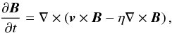 (30)describes the time evolution of a magnetic
field B, where v is the
velocity and η the magnetic diffusivity (25). An arbitrary magnetic field can, in general, be separated into
a mean component B0 and a fluctuating component
δB with
(30)describes the time evolution of a magnetic
field B, where v is the
velocity and η the magnetic diffusivity (25). An arbitrary magnetic field can, in general, be separated into
a mean component B0 and a fluctuating component
δB with 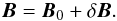 (31)Substituting (31) into the induction equation leads to two equations: an equation
for the large-scale field evolution and the Kazantsev equation (Kazantsev 1968; Brandenburg &
Subramanian 2005), which describes the small-scale evolution of the field.
(31)Substituting (31) into the induction equation leads to two equations: an equation
for the large-scale field evolution and the Kazantsev equation (Kazantsev 1968; Brandenburg &
Subramanian 2005), which describes the small-scale evolution of the field.
The derivation of the Kazantsev equation is based on the assumption that the
fluctuations of the magnetic field as well as the fluctuations of the velocity field are
homogeneous and isotropic even if the mean fields are not isotropic. Furthermore, the
fluctuations are assumed to be Gaussian with a zero mean and the velocity fluctuations
are thought to be δ-correlated in time. For simplicity, any helicity of
the magnetic field is neglected. With these assumptions the Kazantsev equation is (Kazantsev 1968) 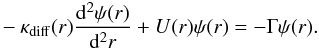 (32)The eigenfunctions of this equation are
related to the longitudinal correlation function of the magnetic fluctuations
ML(r,t) by
(32)The eigenfunctions of this equation are
related to the longitudinal correlation function of the magnetic fluctuations
ML(r,t) by
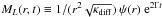 . We call Γ the growth rate of the
small-scale magnetic field. The function κdiff is the
magnetic diffusion coefficient, which contains besides the magnetic diffusivity
η also a scale-dependent turbulent diffusivity. U is
called the “potential” of the Kazantsev equation. Both κdiff
and U only depend on the correlation function of the turbulent velocity
field and the magnetic diffusivity (Subramanian
1997; Schober et al. 2012b).
. We call Γ the growth rate of the
small-scale magnetic field. The function κdiff is the
magnetic diffusion coefficient, which contains besides the magnetic diffusivity
η also a scale-dependent turbulent diffusivity. U is
called the “potential” of the Kazantsev equation. Both κdiff
and U only depend on the correlation function of the turbulent velocity
field and the magnetic diffusivity (Subramanian
1997; Schober et al. 2012b).
The correlation function of the turbulent velocity field in turn depends on the
different types of turbulence, which can be distinguished by the slope of the velocity
spectrum ϑ in the inertial range, where
 (33)Here δv is the velocity of
the fluctuations on the scale ℓ. The range of ϑ goes
from incompressible Kolmogorov turbulence with ϑ = 1/3 (Kolmogorov 1941) to highly compressible Burgers
turbulence with ϑ = 1/2 (Burgers
1948). The gas motions during structure formation have high Mach numbers and
thus the gas gets strongly compressed within shocks. Observations within present-day
molecular clouds by Larson (1981) show that the
slope of the turbulence spectrum is ϑ ≈ 0.38 and thus deviates from
Kolmogorov turbulence. However, other studies (Solomon
et al. 1987; Ossenkopf & Mac Low
2002; Heyer & Brunt 2004) find a
slope of roughly 0.5, whereas Roman-Duval et al.
(2011) show that the variance of ϑ is very large. For our
fiducial model we choose a value of ϑ = 0.4, which lies in between the
extremes.
(33)Here δv is the velocity of
the fluctuations on the scale ℓ. The range of ϑ goes
from incompressible Kolmogorov turbulence with ϑ = 1/3 (Kolmogorov 1941) to highly compressible Burgers
turbulence with ϑ = 1/2 (Burgers
1948). The gas motions during structure formation have high Mach numbers and
thus the gas gets strongly compressed within shocks. Observations within present-day
molecular clouds by Larson (1981) show that the
slope of the turbulence spectrum is ϑ ≈ 0.38 and thus deviates from
Kolmogorov turbulence. However, other studies (Solomon
et al. 1987; Ossenkopf & Mac Low
2002; Heyer & Brunt 2004) find a
slope of roughly 0.5, whereas Roman-Duval et al.
(2011) show that the variance of ϑ is very large. For our
fiducial model we choose a value of ϑ = 0.4, which lies in between the
extremes.
With a model for the turbulent correlation function, the Kazantsev Eq. (32) can be solved with the WKB-approximation
for very large and low Pm. This method is named after Wentzel, Kramers and Brillouin and
is used to find approximative solutions for Schrödinger-type differential equations. In
our model we are in the limit of the very high Pm, where Schober et al. (2012b) find the growth rate 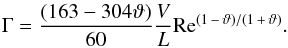 (34)Here V is the typical
velocity on the largest scale of the turbulent eddies of size L. By
solving the Kazantsev Eq. (32)
numerically, Bovino et al. (2013) have recently
confirmed that Eq. (34) describes the
growth rate of the dynamo in the limit large Pm. For our fiducial model with
ϑ = 0.4 the growth rate thus scales with Re0.43.
(34)Here V is the typical
velocity on the largest scale of the turbulent eddies of size L. By
solving the Kazantsev Eq. (32)
numerically, Bovino et al. (2013) have recently
confirmed that Eq. (34) describes the
growth rate of the dynamo in the limit large Pm. For our fiducial model with
ϑ = 0.4 the growth rate thus scales with Re0.43.
2.4.2. Nonlinear small-scale dynamo
As soon as the magnetic energy is comparable to the kinetic energy of the turbulence on
the viscous scale the exponential growth comes to an end. We label this point in time
tν. The dynamo is then saturated on the
viscous scale and the nonlinear growth begins. In this phase the magnetic energy
Emag on the scale of fastest amplification
ℓa evolves as (Schekochihin et al. 2002) 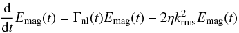 (35)with the nonlinear growth rate
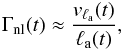 (36)and
 (37)Schleicher
et al. (2013) find that further evaluation of Eq. (35) yields
(37)Schleicher
et al. (2013) find that further evaluation of Eq. (35) yields
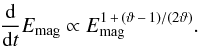 (38)Thus, in the case of Kolmogorov turbulence
with ϑ = 1/3 the magnetic energy grows linear in time, while it grows
quadratically in case of Burgers turbulence with ϑ = 1/2. In our
fiducial model, where we assume ϑ = 0.4, we find
Emag ∝ t4/3 on
ℓa.
(38)Thus, in the case of Kolmogorov turbulence
with ϑ = 1/3 the magnetic energy grows linear in time, while it grows
quadratically in case of Burgers turbulence with ϑ = 1/2. In our
fiducial model, where we assume ϑ = 0.4, we find
Emag ∝ t4/3 on
ℓa.
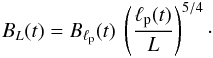
In the nonlinear phase the dynamo process shifts the magnetic energy to larger scales
with the peak scale evolving as 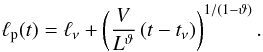 (39)From the peak scale to larger scales we
assume the spectrum to drop off with the Kazantsev slope. By this we can determine the
magnetic field on the forcing scale L at each point in time as
(39)From the peak scale to larger scales we
assume the spectrum to drop off with the Kazantsev slope. By this we can determine the
magnetic field on the forcing scale L at each point in time as
 (40)The nonlinear growth phase comes to an end,
when saturation on the turbulent forcing scale is achieved. Now the spectrum of the
magnetic energy density scales as the one of the kinetic energy density.
(40)The nonlinear growth phase comes to an end,
when saturation on the turbulent forcing scale is achieved. Now the spectrum of the
magnetic energy density scales as the one of the kinetic energy density.
2.4.3. Saturation magnetic field strength from dynamo amplification
A turbulent dynamo can amplify magnetic fields at most to equipartition with the turbulent kinetic energy. However, high-resolution simulations by Federrath et al. (2011a) show that only a certain fraction f of the turbulent kinetic energy can be transformed into magnetic energy. This fraction depends on the type of forcing as well as on the Mach number ℳ. We show f(ℳ) for solenoidal and compressive forcing of turbulence in Fig. 3. Note, that the efficiency of the small-scale dynamo in case of compressive forcing peaks at a Mach number of 1, i.e. at the transition from the subsonic to the supersonic regime. At this point shocks appear, which generate solenoidal motions that are more efficient for dynamo amplification. At larger Mach numbers the efficiency decreases again and appears to become constant.
According to Federrath et al. (2010) solenoidal forcing leads to a slope of the turbulence spectrum of 0.43, while compressive forcing results in ϑ ≈ 0.47. For our fiducial model we choose the saturation efficiency of solenoidal driven turbulence, as we assume a spectrum with ϑ = 0.4.
The resulting saturation magnetic field strength on the forcing scale is
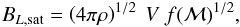 (41)where V is again the
velocity at the forcing scale. If we scale down the turbulent velocity to the viscous
scale by
(41)where V is again the
velocity at the forcing scale. If we scale down the turbulent velocity to the viscous
scale by 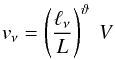 (42)the saturation magnetic field strength on
the viscous scale is
(42)the saturation magnetic field strength on
the viscous scale is 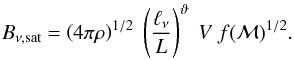 (43)
(43)
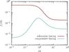 |
Fig. 3 Ratio of magnetic over turbulent kinetic energy at saturation f(ℳ) as a function of the Mach number ℳ. We present fits for solenoidal (solid line) and compressive forcing (dashed line) of the turbulence from the driven MHD simulations by Federrath et al. (2011a). |
2.4.4. Evolution of a magnetic field amplified by the small-scale dynamo
Summarizing the results of this section gives for the magnetic field evolution on the
viscous scale 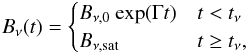 (44)i.e. it grows exponentially with the rate
(34) until saturation on the viscous
scale is reached at the time tν.
(44)i.e. it grows exponentially with the rate
(34) until saturation on the viscous
scale is reached at the time tν.
The field on the turbulent forcing scale evolves as 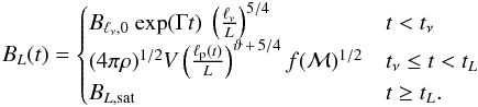 (45)Until the time
tν the field grows exponentially in the
kinematic phase. For
t ≥ tν the dynamo is in
the nonlinear phase, in which the peak of the magnetic spectrum, which is given by Eq.
(39), is shifted toward larger scales.
The dynamo is saturated on all scales of the turbulent inertial range including the
driving scale for times
t ≥ tL.
(45)Until the time
tν the field grows exponentially in the
kinematic phase. For
t ≥ tν the dynamo is in
the nonlinear phase, in which the peak of the magnetic spectrum, which is given by Eq.
(39), is shifted toward larger scales.
The dynamo is saturated on all scales of the turbulent inertial range including the
driving scale for times
t ≥ tL.
The dynamo amplification of a weak magnetic seed field of 10-20 G is shown in Fig. 4. We choose here a forcing scale of 103 pc, which is the radius of the spherical halo considered here, and three different turbulent velocities: 1 km s-1, 10 km s-1 and 100 km s-1. The microphysical quantities are taken from the calculations in the previous sections. In the figure the dashed lines represent the magnetic field strength on the viscous scale, the solid lines the one on the forcing scale.
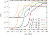 |
Fig. 4 Evolution of the magnetic field amplified by the small-scale dynamo. The dashed lines show the evolution on the viscous scale ℓν, the solid lines the one on the forcing scale of the turbulence L. We use in this plot L = 103 pc. The different colors indicate different turbulent velocities: the red lines have velocities of 1 km s-1, the green lines 10 km s-1 and the orange lines 100 km s-1. The microphysical quantities are determined in Sect. 2.2. The viscosity is ν = 8.7 × 1015 cm2 s-1, the magnetic resistivity η = 37.8 cm2 s-1, the density is n = 10 cm-3 and the mean particle mass is m = 1.6 × 10⁻²⁴ g. The initial magnetic field strength on the viscous scale in this plot is B0 = 10-20 G and the slope of the turbulence spectrum ϑ is 0.4. |
Characteristic quantities of the small-scale dynamo for accretion-driven turbulence (left hand side) and for SN-driven turbulence (right hand side).
3. Magnetic field evolution in a protogalaxy
3.1. Magnetic fields from an accretion-driven small-scale dynamo
3.1.1. Forcing turbulence by accretion
Accretion in a spherical galaxy. During the formation of the primordial halo turbulence
is generated by accretion (Birnboim & Dekel
2003; Semelin & Combes 2005; Wise et al. 2008; Vogelsberger et al. 2013). Simulations show that accretion flows have high
Mach numbers with respect to the cold gas even in the central regions of the halo (Greif et al. 2008). The characteristic forcing scale
in case of a spherical halo is the radius, where the accretion flow comes to a halt:
 (46)Latif et
al. (2013) show in their simulation of a nearly isothermal protogalaxy that the
Mach number in such environment is roughly 2. Thus, the typical turbulent velocities
from accretion are on the order of
(46)Latif et
al. (2013) show in their simulation of a nearly isothermal protogalaxy that the
Mach number in such environment is roughly 2. Thus, the typical turbulent velocities
from accretion are on the order of 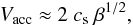 (47)where
cs = (γkT/m)1/2
is the sound speed and we use an adiabatic index γ of 5/3. Further, we
assume here that only a certain fraction β of the kinetic energy of the
accretion flows goes into turbulence, with β typically depending on the
density contrast between the accretion flows and the halo (Klessen & Hennebelle 2010). Simulations (Latif et al. 2013) indicate that about five percent of the kinetic
energy are in turbulent motions, i.e. β ≈ 0.05.
(47)where
cs = (γkT/m)1/2
is the sound speed and we use an adiabatic index γ of 5/3. Further, we
assume here that only a certain fraction β of the kinetic energy of the
accretion flows goes into turbulence, with β typically depending on the
density contrast between the accretion flows and the halo (Klessen & Hennebelle 2010). Simulations (Latif et al. 2013) indicate that about five percent of the kinetic
energy are in turbulent motions, i.e. β ≈ 0.05.
The resulting turbulent length scales, velocities and Reynolds numbers for a spherical galaxy are given in Table 1.
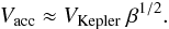
Accretion in a disk-like galaxy. In the case of a disk-like galaxy we adopt the typical
forcing scale of the turbulence by accretion flows to be the scale height
 (48)We further estimate the typical velocity
for accretion flows to be on the order of the Kepler velocity in a disk
(48)We further estimate the typical velocity
for accretion flows to be on the order of the Kepler velocity in a disk  (49)If a percentage β of the
kinetic energy goes into turbulence, the resulting turbulent velocity is given by
(49)If a percentage β of the
kinetic energy goes into turbulence, the resulting turbulent velocity is given by
 (50)Typical values of the length scale, the
velocity scales and the Reynolds numbers with a value of β = 0.05 are
summarized in Table 1.
(50)Typical values of the length scale, the
velocity scales and the Reynolds numbers with a value of β = 0.05 are
summarized in Table 1.
3.1.2. Accretion-driven small-scale dynamo
 |
Fig. 5 Dependency of the accretion-driven small-scale dynamo mechanism on the percentage of kinetic energy that goes into turbulence β. The upper panel shows the different length scales, the middle panel the time until saturation, i.e. tν and tL, and the lower panel the saturation magnetic field strength Bsat. We plot all quantities on the viscous scale ℓν and on the turbulent forcing scale L as indicated in the figure. The solid blue lines show the results for a spherical galaxy, the dashed red lines the ones for a disk. |
Based on the discussion of the strength of magnetic seed fields in the introduction, we
assume the initial magnetic field strength on the viscous scale to be
 (51)This is a rather conservative estimate.
The small-scale dynamo amplifies this seed field as soon as sufficient turbulence has
evolved. The typical growth rates in the kinematic phase are summarized in Table 1. We find 150 Myr-1 for the case of a
spherical galaxy and 1400 Myr-1 for a disk. A fraction of the magnetic energy
can be dissipated again by Ohmic diffusion. The dissipation rate on the viscous scale
ℓν is given by
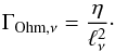 (52)In our model
ΓOhm,ν is on the order of
10-12−10-10 Myr-1 and thus can be neglected compared
the growth rate of the magnetic field.
(52)In our model
ΓOhm,ν is on the order of
10-12−10-10 Myr-1 and thus can be neglected compared
the growth rate of the magnetic field.
With these relatively large growth rates, the small-scale dynamo amplification works on very short timescales. We find that in a spherical galaxy a magnetic field of 1.6 × 10⁻⁶ G and be reached on a scale of 103 pc after 270 Myr. In a disk the saturation field strength is larger by a factor of more than 2. However, the field is only on a scale of 240 pc, but it is saturated after already 24 Myr.
The efficiency of the small-scale dynamo, i.e. the saturation magnetic field strength (Bsat,ν or Bsat,L) that can be achieved and the time on which saturation occurs (tν or tL), depends strongly on the amount of turbulent kinetic energy, controlled by the parameter β (see Eqs. (47) and (50)). In our fiducial model we use β = 0.05, however, this is a rough assumption. We test how the dynamo efficiency changes when varying β in Fig. 5.
In the upper panel of Fig. 5 we show the
dependency of the viscous scale ℓν and the
forcing scale L on β. Of course L is
not effected by β, while
ℓν, which is a function of the Reynolds
number and thus of the turbulent velocity, decreases with increasing β.
The time until saturation of the dynamo, which is shown in the middle panel of Fig.
5, also decreases with increasing
β. This is a natural consequence of the larger amount of turbulent
kinetic energy. In the same way the plot in the lower panel can be understood: the more
turbulent energy, i.e. the higher β, the higher is the saturation field
strength. The magnetic field strength on the forcing scale
Bsat,L increases as
 (53)
(53)
3.2. Magnetic fields from stellar feedback
3.2.1. Distributing stellar magnetic fields by supernovae
A natural source for magnetic fields in the ISM of galaxies are stellar magnetic fields that get distributed over large volumes by SN explosions. Schober et al. (2012a) have shown that the small-scale dynamo can produce strong magnetic fields during primordial star formation. Hints to dynamical important magnetic fields during the formation of the first stars also come from high-resolution numerical simulations (Federrath et al. 2011b; Turk et al. 2012; Sur et al. 2012) and further semi-analytical calculations (Schleicher et al. 2010). Thus, we expect the first and second generations of stars to be magnetized.
Properties of supernova candidates. We assume that a typical star that ends in a
supernova has a mass of  (54)and a radius of
 (55)with the solar mass
M⊙ = 2 × 1033 g and radius
R⊙ = 7 × 1010 cm.
(55)with the solar mass
M⊙ = 2 × 1033 g and radius
R⊙ = 7 × 1010 cm.
It is very difficult to estimate the magnetic energy in a typical population III star,
as there is not much theoretical work on that topic so far. In principle, one could
assume that a certain percentage of the total energy of the SN energy is within the
magnetic field. If the magnetic energy 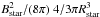 equals e.g., 0.001
ESN, the stellar magnetic field would have a very high
value of Bstar = 8 × 10⁶ G.
equals e.g., 0.001
ESN, the stellar magnetic field would have a very high
value of Bstar = 8 × 10⁶ G.
Here, however, we use as a crude estimate for the magnetic field of population III
stars based on observations of present-day massive stars. In most high-mass stars no
magnetic fields are detected, there are few percent of stars with an enhanced magnetic
field (see Donati & Landstreet 2009). These
so-called “peculiar A or B” stars have a typical dipole field strength of
 (56)We take this value as an upper limit of
magnetic fields in primordial stars, but also test lower stellar field strengths in the
following.
(56)We take this value as an upper limit of
magnetic fields in primordial stars, but also test lower stellar field strengths in the
following.
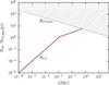 |
Fig. 6 The red line shows the radius of a SN shock RSN(t) as a function of time. Up to roughly 100 yr the SN shock expands freely, then the Sedov-Taylor expansion sets in. The available maximum radius for SNe RSN,max(t) as a function of time is shown for the case of a spherical halo by the blue line. This radius decreases in time, as the number of SN in the protogalactic core increases. The first SN shocks collide after a time of approximately 0.36 Myr. |
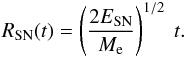
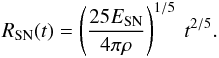
Evolution of a supernova remnant. Stars with masses above 8
M⊙ are expected to explode as a core-collapse supernova,
introducing additional turbulent energy into the ISM (Choudhuri 1998; Padmanabhan 2001).
Initially the shock front of a SN expands freely, i.e. the pressure of the surrounding
ISM is negligible. The shock velocity ve can then be
determined by  (57)where ESN is
the energy of a SN (neglecting the energy loss by neutrinos) and
Me the ejected mass. The shock radius
RSN as a function of time t is thus
(57)where ESN is
the energy of a SN (neglecting the energy loss by neutrinos) and
Me the ejected mass. The shock radius
RSN as a function of time t is thus
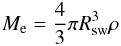
 (58)The free expansion phase ends, when the
accumulated mass of the ISM in front of the shock is of order of
Me. This happens at the so-called sweep-up radius
Rsw defined by
(58)The free expansion phase ends, when the
accumulated mass of the ISM in front of the shock is of order of
Me. This happens at the so-called sweep-up radius
Rsw defined by
 (59)with ρ being the mean
density of the ISM. The shock front reaches Rsw at a time
(59)with ρ being the mean
density of the ISM. The shock front reaches Rsw at a time
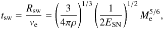 (60)which is in our model on the order of 100
yr. For t > tsw the expansion of the
supernova remnant is driven adiabatically by thermal pressure, which is known as the
Sedov-Taylor phase (Sedov 1946, 1959; Taylor
1950). We can estimate the radius of the shock in this case with
(60)which is in our model on the order of 100
yr. For t > tsw the expansion of the
supernova remnant is driven adiabatically by thermal pressure, which is known as the
Sedov-Taylor phase (Sedov 1946, 1959; Taylor
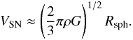
1950). We can estimate the radius of the shock in this case with 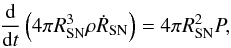 (61)where the
 indicates a time derivative and the
pressure P is given by
indicates a time derivative and the
pressure P is given by
 (62)with γ = 5/3 for adiabatic
expansion. We can solve Eq. (61) with a
simple power-law ansatz and find
(62)with γ = 5/3 for adiabatic
expansion. We can solve Eq. (61) with a
simple power-law ansatz and find
 (63)Thus, the evolution of the SN remnant can
be described by (Choudhuri 1998)
(63)Thus, the evolution of the SN remnant can
be described by (Choudhuri 1998) 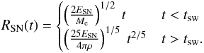 (64)We assume now that the energy released in a
SN explosion is ESN = 1051 erg and that about 10
percent of the mass of the progenitor star is ejected, i.e.
Me ≈ 0.1 Mstar. In our model
the SN remnants evolve as described in Eq. (64) and shown in Fig. 6 until they
collide. At later stages of shock evolution other energy loss mechanisms become
dominant. The electrons lose their energy by ionization, bremsstrahlung, synchrotron
emission and inverse Compton scattering. The latter is the most important energy loss
channel at high redshifts as here the density of the CMB photons is considerably larger
(Schleicher & Beck 2013).
(64)We assume now that the energy released in a
SN explosion is ESN = 1051 erg and that about 10
percent of the mass of the progenitor star is ejected, i.e.
Me ≈ 0.1 Mstar. In our model
the SN remnants evolve as described in Eq. (64) and shown in Fig. 6 until they
collide. At later stages of shock evolution other energy loss mechanisms become
dominant. The electrons lose their energy by ionization, bremsstrahlung, synchrotron
emission and inverse Compton scattering. The latter is the most important energy loss
channel at high redshifts as here the density of the CMB photons is considerably larger
(Schleicher & Beck 2013).
If the SNe are distributed homogeneously in the protogalaxy, each SN shell has a mean
maximum radius at the first collision of 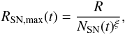 (65)where the radius of the galaxy
R is given in Eqs. (6)
and (9) and the exponent
ξ depends on the geometry of the galaxy. In case of a spherical halo
ξ = 1/3, in case of a thin disk ξ = 1/2. The maximum
expansion radius of the SN shock is shown in Fig. 6
for the spherical case.
(65)where the radius of the galaxy
R is given in Eqs. (6)
and (9) and the exponent
ξ depends on the geometry of the galaxy. In case of a spherical halo
ξ = 1/3, in case of a thin disk ξ = 1/2. The maximum
expansion radius of the SN shock is shown in Fig. 6
for the spherical case.
By comparing (64) to (65) we find the typical time scale for SN
collisions tSN. At that point the SN bubbles fill
approximately the whole galaxy. In the spherical case we find
 (66)which we take as the typical timescale for
SN collisions. Further, we use
RSN(tSN) as the typical length
scale of SN shocks.
(66)which we take as the typical timescale for
SN collisions. Further, we use
RSN(tSN) as the typical length
scale of SN shocks.
Magnetic field evolution. If now all the stellar magnetic energy is distributed into
the volume available by the SN explosion and no significant magnetic energy is left in
the stellar remnant, the resulting magnetic field strength in the ISM after the first SN
generation is 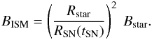 (67)Here, we assumed a spherical shape of the
galaxy and flux freezing. All the following stars will produce roughly the same amount
of magnetic energy, that is then distributed in the ISM by SN. Thus, the time evolution
of the stellar magnetic fields in galaxies can be approximated by
(67)Here, we assumed a spherical shape of the
galaxy and flux freezing. All the following stars will produce roughly the same amount
of magnetic energy, that is then distributed in the ISM by SN. Thus, the time evolution
of the stellar magnetic fields in galaxies can be approximated by
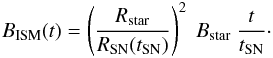 (68)The values of
RSN(tSN) and
tSN depend obviously on the SN rate, which is determined
by the parameter α as defined in (28). We obtain for the spherical case:
(68)The values of
RSN(tSN) and
tSN depend obviously on the SN rate, which is determined
by the parameter α as defined in (28). We obtain for the spherical case:
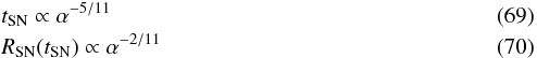
leading to a dependency of the magnetic field distributed by SN on the efficiency of
the SN rate of 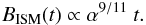 (71)In Fig. 7 we show the evolution of the distributed magnetic fields for different mean
magnetic fields of the stars (104 to 102 G) and for our fiducial
case of α ≈ 0.01. Note that the case of 104 G is an upper
limit of magnetic fields in massive stars. We assume the magnetic fields of the first
stars to be considerably lower.
(71)In Fig. 7 we show the evolution of the distributed magnetic fields for different mean
magnetic fields of the stars (104 to 102 G) and for our fiducial
case of α ≈ 0.01. Note that the case of 104 G is an upper
limit of magnetic fields in massive stars. We assume the magnetic fields of the first
stars to be considerably lower.
The distribution of stellar magnetic fields by SNe explosions thus does not seem to be
important compared to the dynamo amplification in the ISM. However, after a sufficient
time the SN could contribute to the magnetic energy in the ISM. If the equipartition
field strength is roughly 10-6 G, the time after which SN distribution
becomes important is 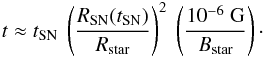 (72)For our fiducial model we find that this
time is about 2.2 × 10⁶ Myr in case of typical stellar field strengths of
104 G. Observations of present-day massive stars indicate that only a few
percent have these high field strengths. We thus also consider the more likely case of
lower mean stellar fields. For a mean strength of 103 G we find that a
micro-Gauss ISM field is only reached after 2.2 × 10⁷ Myr and for a mean
strength of 102 G after 2.2 × 10⁸ Myr. Thus, the typical
timescales of distribution of stellar magnetic fields by supernovae exceed the age of
the Universe by many orders of magnitude and this process cannot be an important
contribution for the fields in the ISM, unless the first stars were much stronger
magnetized than the present-day stars.
(72)For our fiducial model we find that this
time is about 2.2 × 10⁶ Myr in case of typical stellar field strengths of
104 G. Observations of present-day massive stars indicate that only a few
percent have these high field strengths. We thus also consider the more likely case of
lower mean stellar fields. For a mean strength of 103 G we find that a
micro-Gauss ISM field is only reached after 2.2 × 10⁷ Myr and for a mean
strength of 102 G after 2.2 × 10⁸ Myr. Thus, the typical
timescales of distribution of stellar magnetic fields by supernovae exceed the age of
the Universe by many orders of magnitude and this process cannot be an important
contribution for the fields in the ISM, unless the first stars were much stronger
magnetized than the present-day stars.
In the case of a flat disk-shaped galaxy, where we assume the parameter ξ in Eq. (65) to be 1/2, the distribution of stellar magnetic fields proceeds marginally faster. Here the typical time until a field strength of 10-6 G in the ISM is reached is roughly a factor of 10 more quickly.
In reality the evolution of magnetic fields in SN shock fronts is of course more complicated. In addition to simple flux freezing further amplification processes can take place. Miranda et al. (1998) argue that in a multiple explosion scenario of structure formation (Ostriker & Cowie 1981; Miranda & Opher 1997) magnetic seed fields on the order of 10-10 G can be produced on galactic scales. In their model a Biermann battery is operating in the shock of SN explosions of the first stars as here unparallel gradients of temperature and density can be established. Recently, Beck et al. (2013) have also analyzed the magnetic field evolution in protogalaxies based on SN explosions with the cosmological N-body code GADGET. They find that a combination of SNe and subsequent magnetic field amplification leads to magnetic field strengths of a few μG, which is comparable to our results, and that the strength of seed field is coupled to the star formation process.
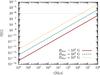 |
Fig. 7 Evolution of the magnetic field, when the only source of magnetic energy in the ISM are stellar magnetic fields distributed by SN explosions. The curves show the results for a spherical halo in our fiducial model with a SN efficiency of α = 0.01. We show three different mean stellar field strengths: 104 G (yellow dotted line), 103 G (green dashed line) and 102 G (solid red line). With the thin gray line we further indicate the typical saturation strength of a magnetic field generated by a small-scale dynamo. |
3.2.2. Dynamo amplification driven by SN turbulence
SN-driven dynamo in a spherical galaxy.
In Sect. 2.3 we discussed the generation of SN turbulence based on numerical simulations. Now we estimate the typical forcing scale LSN and the fluctuation velocity on that scale VSN in order to determine the Reynolds number (1) and the resulting growth rate of the kinematic small-scale dynamo (34). For that we assume that the turbulence driving in the galaxy is in equilibrium.
Then the turbulent pressure, which is roughly 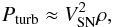 (73)balances the hydrostatic pressure
P determined by
(73)balances the hydrostatic pressure
P determined by 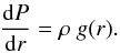 (74)The gravitational acceleration in the
spherical case is roughly
(74)The gravitational acceleration in the
spherical case is roughly  . Solving Eq. (74) and setting it equal to Eq. (73) yields the turbulent velocity
VSN. We find in the spherical case:
. Solving Eq. (74) and setting it equal to Eq. (73) yields the turbulent velocity
VSN. We find in the spherical case:
 (75)The forcing length scale can be estimated
by comparing the energy input rate with the dissipation rate:
(75)The forcing length scale can be estimated
by comparing the energy input rate with the dissipation rate:
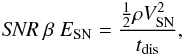 (76)where the dissipation timescale is
 (77)and SNR is the supernova
rate (28). Thus, we find the typical
forcing scale of SN-driven turbulence
(77)and SNR is the supernova
rate (28). Thus, we find the typical
forcing scale of SN-driven turbulence 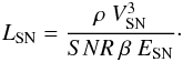 (78)As in the case of the accretion-driven
small-scale dynamo we start with an initial magnetic field strength on the viscous scale
of
(78)As in the case of the accretion-driven
small-scale dynamo we start with an initial magnetic field strength on the viscous scale
of 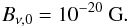 (79)The turbulence driven by SN shocks makes
dynamo action possible, which leads to rapid amplification of the seed field according
to Eqs. (44) and (45). For the case of a spherical galaxy we
find that the growth rate in the kinematic amplification phase is
7.1 × 10³ Myr-1. After a time of 15 Myr the saturation field
strength of 2.1 × 10⁻⁵ G is reached on the forcing scale. The characteristic
quantities of our fiducial models for the SN-driven dynamo are summarized in the right
part of Table 1.
(79)The turbulence driven by SN shocks makes
dynamo action possible, which leads to rapid amplification of the seed field according
to Eqs. (44) and (45). For the case of a spherical galaxy we
find that the growth rate in the kinematic amplification phase is
7.1 × 10³ Myr-1. After a time of 15 Myr the saturation field
strength of 2.1 × 10⁻⁵ G is reached on the forcing scale. The characteristic
quantities of our fiducial models for the SN-driven dynamo are summarized in the right
part of Table 1.
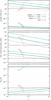 |
Fig. 8 Dependency of the SN-driven small-scale dynamo mechanism on the percentage of kinetic energy that goes into turbulence β and the SN efficiency α. The upper panel shows the different length scales, the middle panel the time until saturation, i.e. tν and tL, and the lower panel the saturation magnetic field strength Bsat. We plot all quantities on the viscous scale ℓν and on the turbulent forcing scale L as indicated in the figure. The dashed-dotted blue line represents the case of a spherical galaxy with α = 0.001, the solid blue line the fiducial case of α = 0.01 and the dotted blue line the case of α = 0.1. The dashed red line shows the results for a disk-like galaxy. There are only 6 lines in the lower plot instead of 8. This results from the fact, that in the spherical case the saturation field strength on the forcing scale does not depend on α nor on β, in contrast to L and tL (see Eqs. (80) to (84)). |
As in case of accretion turbulence, the efficiency of the small-scale dynamo is sensible to the amount of kinetic energy that goes into turbulence β. Moreover, when modeling the scale of turbulence forcing we add another uncertainty namely the supernova rate, which includes the efficiency parameter α (see Eq. (28)). In our fiducial model we choose α = 0.01, but there could easily be a variation of a factor 10. The dependency of the quantities most important for the dynamo amplification on α and β in case of a spherical halo is the following:
![Mathematical equation: \begin{eqnarray} && \ell_{\nu,\mathrm{SN}} \propto \left(\alpha \beta\right)^{-0.28} \\[2mm] && L_\mathrm{SN} \propto \left(\alpha \beta\right)^{-1} \\[2mm] && V_\mathrm{SN} = \mathrm{const.} \\[2mm] && B_{\nu,\mathrm{sat,SN}} \propto \left(\alpha \beta\right)^{0.28} \\[2mm] && B_{L,\mathrm{sat,SN}} = \mathrm{const.} \label{quantities} \end{eqnarray}](/articles/aa/full_html/2013/12/aa22185-13/aa22185-13-eq284.png)
We show the dependency of the length scales, the time until saturation and the saturation magnetic field strength on β and for different values of α in Fig. 8.
SN-driven dynamo in a disk-like galaxy. We perform the same analysis for the disk case.
Here the gravitational acceleration becomes independent of the radius for a thin disk,
i.e. Hdisk ≪ r. In that approximation we
find
g(r) ≈ 2πρGHdisk,
which leads to a turbulent velocity of
 (85)The forcing scale can be determined by Eq.
(78). In case of a disk-shaped galaxy
we find that the typical forcing scale
LSN
(85)The forcing scale can be determined by Eq.
(78). In case of a disk-shaped galaxy
we find that the typical forcing scale
LSN (86)We find that the kinematic growth rate in
our fiducial model is 1.9 × 10⁴ Myr-1. The time until saturation
on the forcing scale is then only 3.8 Myr and the saturation field strength is
2.7 × 10⁻⁵ G.
(86)We find that the kinematic growth rate in
our fiducial model is 1.9 × 10⁴ Myr-1. The time until saturation
on the forcing scale is then only 3.8 Myr and the saturation field strength is
2.7 × 10⁻⁵ G.
In case of a disk-shaped galaxy all the quantities (79) to (84) are independent of α and β. For comparison with the spherical galaxy we show them, however, also in Fig. 8.
4. Conclusions
In this paper we model the evolution of the (turbulent) magnetic field in a young galaxy. We find that weak magnetic seed fields get amplified very efficiently by the small-scale dynamo (see Table 1), which is driven by turbulence from accretion and from supernova (SN) explosions. Dynamo theory predicts that the magnetic field is amplified in two phases: in the kinematic phase the field grows exponentially until the dynamo is saturated on the viscous scale. Then the nonlinear phase begins, where the magnetic energy is shifted toward larger scales until saturation on the turbulent forcing scale occurs.
For our fiducial models of a young galaxy we use a fixed particle density of 10 cm-3 and a temperature of 5 × 10³ K. We concentrate on two different geometries: a spherical and a disk-shaped galaxy (see Sect. 2.1). We determine the viscosity of the plasma, which becomes anisotropic when the plasma becomes magnetized, and the magnetic diffusivity. Turbulence is generated by accretion flows onto the galactic core and also by SN shocks. By estimating typical driving scales and velocities we can determine the hydrodynamic and the magnetic Reynolds number. The magnetic field evolution depends strongly on the type of turbulence, which we assume to be a mixture of solenoidal and compressive modes.
For our fiducial model we find that the dynamo saturates on the largest scale in accretion-driven turbulence after a time of roughly 270 Myr in case of a spherical galaxy and after 24 Myr in case of a disk. Turbulence generated by SN shocks can amplify the magnetic field on shorter timescales, with saturation reached after 15 Myr in a spherical galaxy and 3.8 Myr in a disk. The dynamo timescale is thus comparable to the free-fall time tff = (3π/(32Gρ))1/2 ≈ 16 Myr. The age of the Universe at the onset of galaxy formation, i.e. at a redshift of 10, is roughly 470 Myr, which is larger than the dynamo timescales by factor of 2 to 120 for our four fiducial models. In the models with the longest amplification times our assumption of constant accretion and supernova rates may thus not be very precise. Nevertheless, these models provide an order of magnitude estimate of the resulting magnetic strength. In case of a disk-like galaxy we can compare the dynamo timescales further to the typical time of one rotation, which turns out to be 340 Myr when using the Kepler velocity (49). Thus, we can expect that the small-scale dynamo is saturated within less then one orbital time, the turbulent magnetic field gets ordered and an α−Ω dynamo, i.e. a galactic large-scale dynamo, sets in. The role of rotation has been analyzed for example by Kotarba et al. (2009) and Kotarba et al. (2011) in numerical simulations and is extremely important for understanding the present-day large-scale structure of galactic magnetic fields.
The magnetic field strengths predicted by our fiducial models are very high with values between 1.6 × 10⁻⁶ G and 4.3 × 10⁻⁶ G in the accretion-driven case and between 2.1 × 10⁻⁵ G and 2.7 × 10⁻⁵ G in the SN-driven case for a spherical galaxy and a disk, respectively. These field strengths are comparable with the ones observed in the local Universe, where the typical turbulent field component in present-day disk galaxies is (2−3) × 10-5 G in spiral arms and bars and up to (5−10) × 10-5 G in the central starburst regions (Beck 2011). New radio observations also detect magnetic fields in dwarf galaxies. Their field strengths, which seem to be correlated with the star formation rate, are typically a factor of three lower compared to the one in spiral galaxies (Chyży et al. 2011).
Our calculations suggest that the turbulent magnetic field of a galaxy was very high already at high redshifts. An observational confirmation of this result is very complicated. A hint toward an early generation of the turbulent magnetic field in galaxies comes from Hammond et al. (2012). They analyze the rotation measure of a huge catalog of extragalactic radio sources as a function of redshift and find that it is constant up to redshifts of 5.3, which is the maximum redshift in their dataset. A very powerful tool provides, moreover, the far-infrared – radio correlation, which relates the star formation rate to the synchrotron loss of cosmic ray electrons. It is observed to be constant up to redshifts of roughly 2 (Sargent et al. 2010; Bourne et al. 2011), but is expected to break down at a higher redshift, which depends on the star formation rate and the evolution of typical ISM densities (Schleicher & Beck 2013). With new instruments like SKA and LOFAR our knowledge about the evolution of the cosmic magnetic fields will increase.
Besides our fiducial models we analyze the effect of changing the amount of kinetic energy that goes into turbulence and find that the dynamo is more efficient with increasing turbulent energy, which is intuitively clear. Furthermore we determine the small-scale dynamo evolution for a varying supernova rate (SNR), which is important for estimating the driving scale of SN turbulence in the case of a spherical core. As expected the time until saturation increases with increasing SNR. However, the typical largest scale of the magnetic field decreases with the supernova rate.
We further estimate the effect of magnetic field enrichment in galaxies by distributing stellar fields by SN explosions. As an estimate of the magnetic energy in the first stars is very hard, we determine the expected magnetic field evolution in the ISM for three different cases. An upper limit of magnetic field strengths of the primordial stars is 104 G, which is a value observed in a the few percent of present-day massive stars that are magnetized. Distributing these mean stellar fields by SNe in the ISM, we find that a ISM field strength of 10-6 G is reached after 106 Myr, which is already longer than the Hubble time. Thus, the dynamo increases the magnetic field strength much faster.
With our model we have shown that the small-scale dynamo can amplify weak magnetic seed fields in the ISM of early galaxies on relatively short time scales compared to other evolutionary timescales. This leads to the build-up of strong magnetic fields already at very early phases of (proto)galactic evolution. Theoretical models of galaxy evolution describe a collapse of a spherical object to a disk. Comparison of the gravitational energy, 3/5GM2R-3 ≈ 1055 erg, with the magnetic energy at dynamo saturation, B2/(8π) ≈ 1053 erg, shows that the field is not strong enough to prevent to collapse. Still the magnetic field produced by the small-scale dynamo has potentially strong impact on ISM dynamics and subsequent star formation.
Acknowledgments
We thank the anonymous referee for useful comments on our manuscript. We acknowledge funding through the Deutsche Forschungsgemeinschaft (DFG) in the Schwerpunktprogramm SPP 1573 “Physics of the Interstellar Medium” under grant KL 1358/14-1 and SCHL 1964/1-1. Moreover, we thank for financial support by the Baden-Württemberg-Stiftung via contract research (grant P-LS-SPII/18) in their program “Internationale Spitzenforschung II” as well as the DFG via the SFB 881 “The Milky Way System” in the sub-projects B1 and B2. J.S. acknowledges the support by IMPRS HD. D.R.G.S. thanks for funding via the SFB 963/1 (project A12) on “Astrophysical flow instabilities and turbulence”.
References
- Abel, T., Bryan, G. L., & Norman, M. L. 2002, Science, 295, 93 [NASA ADS] [CrossRef] [PubMed] [Google Scholar]
- Balsara, D. S., Kim, J., Mac Low, M.-M., & Mathews, G. J. 2004, ApJ, 617, 339 [NASA ADS] [CrossRef] [Google Scholar]
- Banerjee, R., & Jedamzik, K. 2004, Phys. Rev. D, 70, 123003 [NASA ADS] [CrossRef] [Google Scholar]
- Beck, A. M., Lesch, H., Dolag, K., et al. 2012, MNRAS, 422, 2152 [NASA ADS] [CrossRef] [Google Scholar]
- Beck, A. M., Dolag, K., Lesch, H., & Kronberg, P. P. 2013, MNRAS, 435, 3575 [NASA ADS] [CrossRef] [Google Scholar]
- Beck, R. 2011, Space Sci. Rev., 135 [Google Scholar]
- Beck, R., Ehle, M., Shoutenkov, V., Shukurov, A., & Sokoloff, D. 1999, Nature, 397, 324 [NASA ADS] [CrossRef] [Google Scholar]
- Bernet, M. L., Miniati, F., Lilly, S. J., Kronberg, P. P., & Dessauges-Zavadsky, M. 2008, Nature, 454, 302 [NASA ADS] [CrossRef] [PubMed] [Google Scholar]
- Biermann, L. 1950, Zeitschrift Naturforschung Teil A, 5, 65 [NASA ADS] [Google Scholar]
- Birnboim, Y., & Dekel, A. 2003, MNRAS, 345, 349 [NASA ADS] [CrossRef] [Google Scholar]
- Bourne, N., Dunne, L., Ivison, R. J., et al. 2011, MNRAS, 410, 1155 [NASA ADS] [CrossRef] [Google Scholar]
- Bovino, S., Schleicher, D. R. G., & Schober, J. 2013, New J. Phys., 15, 013055 [NASA ADS] [CrossRef] [Google Scholar]
- Braginskii, S. I. 1965, Rev. Plasma Phys., 1, 205 [NASA ADS] [Google Scholar]
- Brandenburg, A., & Subramanian, K. 2005, Phys. Rep., 417, 1 [NASA ADS] [CrossRef] [Google Scholar]
- Bromm, V., & Larson, R. B. 2004, ARA&A, 42, 79 [NASA ADS] [CrossRef] [EDP Sciences] [Google Scholar]
- Bromm, V., & Yoshida, N. 2011, ARA&A, 49, 373 [NASA ADS] [CrossRef] [Google Scholar]
- Bromm, V., Yoshida, N., Hernquist, L., & McKee, C. F. 2009, Nature, 459, 49 [NASA ADS] [CrossRef] [PubMed] [Google Scholar]
- Burgers, J. 1948, Adv. Appl. Mech., 1, 171 [CrossRef] [MathSciNet] [Google Scholar]
- Chapman, S., Cowling, T., & Társulat, M. T. 1953, The Mathematical Theory of Non-uniform Gases: An Account of the Kinetic Theory of Viscosity, Thermal Conduction and Diffusion in Gases. Prepared in Co-operation with D. Burnet (University Press) [Google Scholar]
- Choudhuri, A. R. 1998, The Physics of Fluids and Plasmas: An Introduction for Astrophysicists (Cambrigde University Press) [Google Scholar]
- Chyży, K. T., Weżgowiec, M., Beck, R., & Bomans, D. J. 2011, A&A, 529, A94 [NASA ADS] [CrossRef] [EDP Sciences] [Google Scholar]
- Clark, P. C., Glover, S. C. O., Smith, R. J., et al. 2011, Science, 331, 1040 [NASA ADS] [CrossRef] [PubMed] [Google Scholar]
- Dekel, A., Birnboim, Y., Engel, G., et al. 2009, Nature, 457, 451 [NASA ADS] [CrossRef] [PubMed] [Google Scholar]
- Donati, J.-F., & Landstreet, J. D. 2009, ARA&A, 47, 333 [NASA ADS] [CrossRef] [MathSciNet] [Google Scholar]
- Federrath, C., Roman-Duval, J., Klessen, R. S., Schmidt, W., & Mac Low, M.-M. 2010, A&A, 512, A81 [NASA ADS] [CrossRef] [EDP Sciences] [Google Scholar]
- Federrath, C., Chabrier, G., Schober, J., et al. 2011a, Phys. Rev. Lett., 107, 114504 [NASA ADS] [CrossRef] [Google Scholar]
- Federrath, C., Sur, S., Schleicher, D. R. G., Banerjee, R., & Klessen, R. S. 2011b, ApJ, 731, 62 [NASA ADS] [CrossRef] [Google Scholar]
- Greif, T. H., Johnson, J. L., Klessen, R. S., & Bromm, V. 2008, MNRAS, 387, 1021 [NASA ADS] [CrossRef] [Google Scholar]
- Hammond, A. M., Robishaw, T., & Gaensler, B. M. 2012 [arXiv:1209.1438] [Google Scholar]
- Heyer, M. H., & Brunt, C. M. 2004, ApJ, 615, 45 [Google Scholar]
- Kazantsev, A. P. 1968, Sov. J. Exp. Theor. Phys., 26, 1031 [Google Scholar]
- Kim, K.-T., Kronberg, P. P., Giovannini, G., & Venturi, T. 1989, Nature, 341, 720 [NASA ADS] [CrossRef] [Google Scholar]
- Klessen, R. S., & Hennebelle, P. 2010, A&A, 520, A17 [NASA ADS] [CrossRef] [EDP Sciences] [Google Scholar]
- Kolmogorov, A. 1941, Akademiia Nauk SSSR Doklady, 30, 301 [Google Scholar]
- Kotarba, H., Lesch, H., Dolag, K., et al. 2009, MNRAS, 397, 733 [NASA ADS] [CrossRef] [Google Scholar]
- Kotarba, H., Lesch, H., Dolag, K., et al. 2011, MNRAS, 415, 3189 [NASA ADS] [CrossRef] [Google Scholar]
- Kronberg, P. P. 1994, Rep. Prog. Phys., 57, 325 [Google Scholar]
- Kulsrud, R. M. & Zweibel, E. G. 2008, Rep. Prog. Phys., 71, 046901 [NASA ADS] [CrossRef] [Google Scholar]
- Larson, R. B. 1981, MNRAS, 194, 809 [NASA ADS] [CrossRef] [Google Scholar]
- Latif, M. A., Schleicher, D. R. G., Schmidt, W., & Niemeyer, J. 2013, MNRAS, 432, 668 [NASA ADS] [CrossRef] [Google Scholar]
- Mac Low, M.-M., & Klessen, R. S. 2004, Rev. Mod. Phys., 76, 125 [NASA ADS] [CrossRef] [Google Scholar]
- McKee, C. F., & Ostriker, E. C. 2007, ARA&A, 45, 565 [NASA ADS] [CrossRef] [Google Scholar]
- Miranda, O. D., & Opher, R. 1997, ApJ, 482, 573 [NASA ADS] [CrossRef] [Google Scholar]
- Miranda, O. D., Opher, M., & Opher, R. 1998, MNRAS, 301, 547 [NASA ADS] [CrossRef] [Google Scholar]
- Murphy, E. J. 2009, ApJ, 706, 482 [NASA ADS] [CrossRef] [Google Scholar]
- Nelson, D., Vogelsberger, M., Genel, S., et al. 2013, MNRAS, 429, 3353 [NASA ADS] [CrossRef] [Google Scholar]
- Neronov, A., Semikoz, D., & Banafsheh, M. 2013 [arXiv:1305.1450] [Google Scholar]
- Ossenkopf, V., & Mac Low, M.-M. 2002, A&A, 390, 307 [NASA ADS] [CrossRef] [EDP Sciences] [Google Scholar]
- Ostriker, J. P., & Cowie, L. L. 1981, ApJ, 243, 127 [NASA ADS] [CrossRef] [Google Scholar]
- Padmanabhan, T. 2001, Theoretical Astrophysics – Volume 2, Stars and Stellar Systems (Cambridge University press) [Google Scholar]
- Rees, M. J. 1987, Q. J. R. Astron. Soc., 28, 197 [Google Scholar]
- Reiners, A. 2012, Liv. Rev. Sol. Phys., 9, 1 [Google Scholar]
- Roman-Duval, J., Federrath, C., Brunt, C., et al. 2011, ApJ, 740, 120 [NASA ADS] [CrossRef] [Google Scholar]
- Sargent, M. T., Schinnerer, E., Murphy, E., et al. 2010, ApJ, 714, 190 [Google Scholar]
- Schekochihin, A. A., Cowley, S. C., Hammett, G. W., Maron, J. L., & McWilliams, J. C. 2002, New J. Phys., 4, 84 [NASA ADS] [CrossRef] [Google Scholar]
- Schleicher, D. R. G., & Beck, R. 2013, A&A, 556, A142 [NASA ADS] [CrossRef] [EDP Sciences] [Google Scholar]
- Schleicher, D. R. G., Banerjee, R., Sur, S., et al. 2010, A&A, 522, A115 [NASA ADS] [CrossRef] [EDP Sciences] [Google Scholar]
- Schleicher, D. R. G., Schober, J., Federrath, C., Bovino, S., & Schmidt, W. 2013, New J. Phys., 15, 023017 [NASA ADS] [CrossRef] [Google Scholar]
- Schlickeiser, R. 2012, Phys. Rev. Lett., 109, 261101 [NASA ADS] [CrossRef] [Google Scholar]
- Schober, J., Schleicher, D., Federrath, C., et al. 2012a, ApJ, 754, 99 [NASA ADS] [CrossRef] [Google Scholar]
- Schober, J., Schleicher, D., Federrath, C., Klessen, R., & Banerjee, R. 2012b, Phys. Rev. E, 85, 026303 [NASA ADS] [CrossRef] [Google Scholar]
- Sedov, L. I. 1946, Dokl. Akad. Nauk. SSSR, 52, 17 [Google Scholar]
- Sedov, L. I. 1959, Similarity and Dimensional Methods in Mechanics (New York: Academic press) [Google Scholar]
- Semelin, B., & Combes, F. 2005, A&A, 441, 55 [NASA ADS] [CrossRef] [EDP Sciences] [Google Scholar]
- Shiraishi, M., Nitta, D., Yokoyama, S., & Ichiki, K. 2012, J. Cosmol. Astropart. Phys., 3, 41 [NASA ADS] [CrossRef] [Google Scholar]
- Sigl, G., Olinto, A. V., & Jedamzik, K. 1997, Phys. Rev. D, 55, 4582 [Google Scholar]
- Simon, A. 1955, Phys. Rev., 100, 1557 [NASA ADS] [CrossRef] [Google Scholar]
- Solomon, P. M., Rivolo, A. R., Barrett, J., & Yahil, A. 1987, ApJ, 319, 730 [NASA ADS] [CrossRef] [Google Scholar]
- Spitzer, L. 1956, Physics of Fully Ionized Gases (New York: Interscience) [Google Scholar]
- Subramanian, K. 1997 [arXiv:astro-ph/9708216] [Google Scholar]
- Sur, S., Federrath, C., Schleicher, D. R. G., Banerjee, R., & Klessen, R. S. 2012, MNRAS, 423, 3148 [NASA ADS] [CrossRef] [Google Scholar]
- Taylor, G. 1950, Roy. Soc. London Proc. Ser. A, 201, 159 [NASA ADS] [Google Scholar]
- Turk, M. J., Oishi, J. S., Abel, T., & Bryan, G. L. 2012, ApJ, 745, 154 [NASA ADS] [CrossRef] [Google Scholar]
- Turner, M. S., & Widrow, L. M. 1988, Phys. Rev. D, 37, 2743 [NASA ADS] [CrossRef] [Google Scholar]
- Vogelsberger, M., Genel, S., Sijacki, D., et al. 2013, MNRAS, submitted [arXiv:1305.2913] [Google Scholar]
- Wise, J. H., Turk, M. J., & Abel, T. 2008, ApJ, 682, 745 [NASA ADS] [CrossRef] [Google Scholar]
- Xu, H., O’Shea, B. W., Collins, D. C., et al. 2008, ApJ, 688, 57 [Google Scholar]
All Tables
Characteristic quantities of the small-scale dynamo for accretion-driven turbulence (left hand side) and for SN-driven turbulence (right hand side).
All Figures
|
Fig. 1 Gyro-radii of electrons and ions ρe and ρp as a function of magnetic field strength compared to the typical macroscopic scale L ≈ 103 pc and the mean-free path ℓmfp. Within our fiducial case for the density and the temperature the electron fluid becomes magnetized at a magnetic field strength of roughly 10-12 G, the ion fluid at 10-10 G. |
| In the text | |
|
Fig. 2 Kinematic viscosity parallel (ν∥) and perpendicular to the magnetic field lines (ν⊥) as a function of magnetic field strength B. We show the results for the electron as well as for the ion fluid. The range between 10-11 G and 10-7 G is not shown, as here the transition from the unmagnetized to a magnetized plasma takes place. |
| In the text | |
|
Fig. 3 Ratio of magnetic over turbulent kinetic energy at saturation f(ℳ) as a function of the Mach number ℳ. We present fits for solenoidal (solid line) and compressive forcing (dashed line) of the turbulence from the driven MHD simulations by Federrath et al. (2011a). |
| In the text | |
|
Fig. 4 Evolution of the magnetic field amplified by the small-scale dynamo. The dashed lines show the evolution on the viscous scale ℓν, the solid lines the one on the forcing scale of the turbulence L. We use in this plot L = 103 pc. The different colors indicate different turbulent velocities: the red lines have velocities of 1 km s-1, the green lines 10 km s-1 and the orange lines 100 km s-1. The microphysical quantities are determined in Sect. 2.2. The viscosity is ν = 8.7 × 1015 cm2 s-1, the magnetic resistivity η = 37.8 cm2 s-1, the density is n = 10 cm-3 and the mean particle mass is m = 1.6 × 10⁻²⁴ g. The initial magnetic field strength on the viscous scale in this plot is B0 = 10-20 G and the slope of the turbulence spectrum ϑ is 0.4. |
| In the text | |
|
Fig. 5 Dependency of the accretion-driven small-scale dynamo mechanism on the percentage of kinetic energy that goes into turbulence β. The upper panel shows the different length scales, the middle panel the time until saturation, i.e. tν and tL, and the lower panel the saturation magnetic field strength Bsat. We plot all quantities on the viscous scale ℓν and on the turbulent forcing scale L as indicated in the figure. The solid blue lines show the results for a spherical galaxy, the dashed red lines the ones for a disk. |
| In the text | |
|
Fig. 6 The red line shows the radius of a SN shock RSN(t) as a function of time. Up to roughly 100 yr the SN shock expands freely, then the Sedov-Taylor expansion sets in. The available maximum radius for SNe RSN,max(t) as a function of time is shown for the case of a spherical halo by the blue line. This radius decreases in time, as the number of SN in the protogalactic core increases. The first SN shocks collide after a time of approximately 0.36 Myr. |
| In the text | |
|
Fig. 7 Evolution of the magnetic field, when the only source of magnetic energy in the ISM are stellar magnetic fields distributed by SN explosions. The curves show the results for a spherical halo in our fiducial model with a SN efficiency of α = 0.01. We show three different mean stellar field strengths: 104 G (yellow dotted line), 103 G (green dashed line) and 102 G (solid red line). With the thin gray line we further indicate the typical saturation strength of a magnetic field generated by a small-scale dynamo. |
| In the text | |
|
Fig. 8 Dependency of the SN-driven small-scale dynamo mechanism on the percentage of kinetic energy that goes into turbulence β and the SN efficiency α. The upper panel shows the different length scales, the middle panel the time until saturation, i.e. tν and tL, and the lower panel the saturation magnetic field strength Bsat. We plot all quantities on the viscous scale ℓν and on the turbulent forcing scale L as indicated in the figure. The dashed-dotted blue line represents the case of a spherical galaxy with α = 0.001, the solid blue line the fiducial case of α = 0.01 and the dotted blue line the case of α = 0.1. The dashed red line shows the results for a disk-like galaxy. There are only 6 lines in the lower plot instead of 8. This results from the fact, that in the spherical case the saturation field strength on the forcing scale does not depend on α nor on β, in contrast to L and tL (see Eqs. (80) to (84)). |
| In the text | |
Current usage metrics show cumulative count of Article Views (full-text article views including HTML views, PDF and ePub downloads, according to the available data) and Abstracts Views on Vision4Press platform.
Data correspond to usage on the plateform after 2015. The current usage metrics is available 48-96 hours after online publication and is updated daily on week days.
Initial download of the metrics may take a while.