| Issue |
A&A
Volume 560, December 2013
|
|
|---|---|---|
| Article Number | A112 | |
| Number of page(s) | 20 | |
| Section | Planets and planetary systems | |
| DOI | https://doi.org/10.1051/0004-6361/201322079 | |
| Published online | 16 December 2013 | |
High-precision stellar limb-darkening measurements
A transit study of 38 Kepler planetary candidates⋆
Hamburger Sternwarte, Universität Hamburg,
Gojenbergsweg 112,
21029
Hamburg,
Germany
e-mail:
This email address is being protected from spambots. You need JavaScript enabled to view it.
Received:
13
June
2013
Accepted:
25
September
2013
Abstract
Context. Planetary transit light curves are influenced by a variety of fundamental parameters, such as the orbital geometry and the surface brightness distribution of the host star. Stellar limb darkening (LD) is therefore among the key parameters of transit modeling. In many applications, LD is presumed to be known and modeled based on synthetic stellar atmospheres.
Aims. We measure LD in a sample of 38 Kepler planetary candidate host stars covering effective temperatures between 3000 K and 8900 K with a range of surface gravities from 3.8 to 4.7. In our study we compare our measurements to widely used theoretically predicted quadratic limb-darkening coefficients (LDCs) to check their validity.
Methods. We carried out a consistent analysis of a unique stellar sample provided by the Kepler satellite. We performed a Markov chain Monte Carlo (MCMC) modeling of low-noise, short-cadence Kepler transit light curves, which yields reliable error estimates for the LD measurements in spite of the highly correlated parameters encountered in transit modeling.
Results. Our study demonstrates that it is impossible to measure accurate LDCs by transit modeling in systems with high impact parameters (b ≳ 0.8). For the majority of the remaining sample objects, our measurements agree with the theoretical predictions, considering measurement errors and mutual discrepancies between the theoretical predictions. Nonetheless, theory systematically overpredicts our measurements of the quadratic LDC u2 by about 0.07. Systematic errors of this order for LDCs would lead to an uncertainty on the order of 1% for the derived planetary parameters.
Conclusions. We find that it is adequate to set the commonly used theoretical LDCs as fixed parameters in transit modeling. Furthermore, it is even indispensable to use theoretical LDCs in the case of transiting systems with a high impact parameter, since the host star’s LD cannot be determined from their transit light curves.
Key words: stars: atmospheres / planetary systems / methods: data analysis / techniques: photometric
Table 3 and appendices are available in electronic form at http://www.aanda.org
© ESO, 2013
1. Introduction
Since the early studies of eclipsing binary light curves the center-to-limb intensity distribution of stellar disks has played an important role in photometric analyses (e.g., Russell & Shapley 1912). For optical wavelengths this distribution shows a darkening toward the stellar limb, which is easily seen on the Sun. This so-called limb darkening (LD) depends on the surface temperature of the underlying stars and is difficult to measure when the stellar disk remains unresolved. In the early stages of LD studies, this intensity trend was theoretically described by a linear formula provided by Schwarzschild (1906). This linear description has been used to model a verity of observed data, such as eclipsing binary light curves, and it is still in use in analyses of the Rossiter-McLaughlin effect (Ohta et al. 2005) or in Doppler imaging (e.g., Nesvacil et al. 2012). More complicated descriptions of LD have been proposed (e.g., Kopal 1950) and adopted by several other authors. Although these models are commonly referred to as limb-darkening “laws”, they are only approximations of the real stellar LD.
When modeling LD in, say, transit light curves, the LD laws are parameterized by some sets of coefficients. These are either left as free fit parameters during data analysis or determined beforehand by model atmospheres and kept fixed in the actual light curve modeling. The determination of LD coefficients (LDCs) for a variety of different laws using model atmospheres has been carried out by many authors (e.g., Wade & Rucinski 1985; van Hamme 1993; Sing 2010; Howarth 2011a; Claret & Bloemen 2011). Whether these theoretical LDCs are used and fixed or freely fitted in light curve models can have significant effects on the results. Although it clearly is preferable to fix parameters in a fit that can be determined in some other way, it is not clear how reliable these theoretical LDCs are. After all, they only represent approximations to model atmospheres. Direct measurements of LD can only be carried out for a few exceptional stars with a spatially resolved surface, such as Betelgeuse (Haubois et al. 2009) using interferometric observations or, most notably, our Sun (Neckel & Labs 1994).
The importance of a correct description of LD was recognized once researchers began to study light curves of transiting extrasolar planets (Charbonneau et al. 2000). Transit light curves are an important tool for studying the physical parameters of exoplanets, such as their radii and densities. Stellar LD is often considered as nuisance parameter in transit modeling, which is strongly correlated to the other model parameters (Carter et al. 2008). Thus, prior knowledge of the LDCs would significantly reduce the uncertainty in the physical parameters of the planets. However, transit light curve analysts have to choose from a variety of LD laws and select appropriate theoretical LDCs. These choices are often quite arbitrary, and incorrect coefficients can introduce large errors in the derived model parameters; this is one of the reasons why many researchers tend to leave their LDCs as free fit parameters.
There is an ongoing debate whether theoretical LDCs and LD laws are accurate enough to describe the real stellar brightness distribution. Today, high-precision transit light curves of planets and eclipsing binaries render it feasible to study stellar LD for a substantial number of stars with high accuracy. Some studies measure LD using eclipsing binary stars (e.g., Heyrovský 2007; Claret 2008) and found disagreements between empirical and predicted LDCs using the linear limb-darkening law. Knutson et al. (2007) note in their study of HD 209458b that even the four parametric nonlinear LD law leads to clear residuals when they use the predicted LDCs. Southworth (2008) used up to five different LD laws in planetary transit models and stated that “the solutions of all but the highest-quality transit light curves are not adversely affected by the choice of LD law”. Southworth also tested the effects of setting LDCs to predicted values for some objects and found that the resulting planetary parameters show no significant differences from leaving the LDCs free; however, he also found the same disagreements for HD 209458A as Knutson et al. (2007). Other authors found further disagreements between theoretical and measured LDCs, as e.g. Kipping & Bakos (2011a) for Kepler-5b, also included in our analysis, and Sing (2010) for seven CoRoT targets. On the one hand these studies seem to suggest that it is necessary to fit the LDCs when modeling light curves, as already claimed by other authors (e.g., Southworth 2008; Csizmadia et al. 2013); on the other hand, there are also objects which show good agreement with the theoretical LDCs (Bordé et al. 2010) and one always has to keep in mind that the determined LDCs usually have rather large errors.
There are 3D hydrodynamic atmospheric models that predict a slightly weaker limb darkening than 1D models, potentially indicating a systematic deficiency of the 1D approach. As demonstrated by Asplund et al. (2009), these 3D models successfully reproduce the solar LD (see also, Trampedach et al. 2013). The deviation between the solar 1D and 3D models compared by Asplund et al. (2009) amounts to roughly 10% in terms of flux at intermediate limb angles in the visible, which corresponds to a 10% deviation in the LDCs. Hayek et al. (2012), who apply similar 3D models to exoplanet host stars, ascribe the weaker limb darkening to a shallower temperature gradient in the photosphere. However, this behavior has not been reproduced in the 3D solar models computed by Hauschildt & Baron (2010), who combine the radiative transfer of the PHOENIX code with a snapshot of a hydrodynamic model of the photosphere (Caffau et al. 2007; Wedemeyer et al. 2004).
In the end, the core question is still not conclusively answered: Are the theoretical LDCs compatible with empirical ones? The aim of this work is to take another step toward a consistent answer to this question. Although today it is hardly possible to directly observe LD for many stars, some dozen light curves of the Kepler space telescope show sufficient precision to indirectly analyze stellar LD with high accuracy. Furthermore, using only one instrument with one spectral response function allows us to consistently analyze the stellar LD with a wide diversity of parameters.
In this paper we present measurements of the quadratic limb-darkening coefficients using high-quality space-based transit light curves of 38 Kepler planetary candidate host stars divided into 26 target stars with highest signal-to-noise ratios (SNRs) and 12 objects with large system impact parameters. We concentrate on how well our determined LDCs agree with the theoretically predicted coefficients from commonly used model atmospheres for main sequence stars (PHOENIX and ATLAS). In Sect. 2 we explain our selection criteria of Kepler objects, our data preparation, and our transit normalization. Section 3 provides information on the used routines, on the modeling approach, and the error analysis. Section 4 is dedicated to objects showing time correlated noise or other anomalies presumably caused by instrumental effects, while in Sect. 5 we present our results and compare them to predictions. In Sect. 6 we summarize our results and provide conclusions concerning the treatment of limb darkening in transit modeling.
2. Data priming and selection of suitable objects
2.1. Target selection
For our analysis we retrieved the Kepler data of quarters Q0 to Q6 from the NASA Mikulski Archive for Space Telescopes (MAST1). Kepler produces photometric light curves in two different sampling modes: long cadence (LC) and short cadence (SC) with sampling rates of about half an hour and one minute, respectively. The data consist of different data releases from release 4 to 7, depending on the quarter and the sampling mode. The raw data have been processed using Kepler’s photometric analysis (PA) pipeline, which includes barycentric time correction, detection of cosmic ray events, and background removal. This leads to the raw aperture photometry (SAP) flux. We used the corrected aperture photometry (PDCSAP) flux for our investigations, which is the result of Kepler’s pre-search data conditioning (PDC) pipeline applied to the raw flux. In addition to the PA, the PDC corrects for systematic errors, such as jumps and exponential decays caused by the instrument, and removes excess flux within the target apertures which could be induced by background or foreground stars in crowded fields or by physically bound companions. Such a third light contribution can affect planet parameters in transit modeling, e.g. mentioned for CoRoT-2b (Alonso et al. 2008) or TrES-2b (Daemgen et al. 2009). Further information on the reduction process is presented in the data release notes provided by the Kepler Data Analysis Working Group2.
As of February 2013, the Kepler space mission has discovered 2321 planetary candidates, 322 of them are observed in SC mode. The false positive rate among the planetary candidates, although still under debate (see Fressin et al. 2013, and references there), appears to be low, of the order of 10%. Due to the longer integration time of LC data, the resulting transit light curves contain less spatial information on the host star than those observed in SC mode. For this reason we restrict our investigation to the planetary candidates recorded in SC mode because we need the highest temporal resolution available to spatially resolve LD on the stellar disk. For all selected light curves we removed invalid data points and all points marked by the SAP_QUALITY flag, and we used Kepler’s TIME axis in BJD (adding the BJDREFI value contained in the FITS-header).
2.1.1. High signal-to-noise target sample
For an appropriate analysis of limb darkening we require transit light curves with
extremely high SNRs, many data points during the occultations, and short orbital periods
to gather as many transits as possible. These are idealized requirements and light
curves combining them are rare in real data sets. We made use of the public released
Kepler planetary candidates list3 (KPCL) to select
light curves which fulfill these conditions best. This list provides each light curve’s
SNR (see Borucki et al. 2011, Table 2 and Chap. 4)
and important system parameters, such as orbital period and transit duration, for all
planetary candidates. To illustrate our selection procedure we show in Fig. 1 the SNR value plotted against the
number of transit data points per day of each object
 ,
where tdur denotes the transit duration and
tcad represents Kepler’s cadence of data
acquisition (≈60 s). Most objects are found at SNR values ≲200 and with
less than 50 transit data points per day. To obtain the most reliable results, we only
select the 26 objects with a SNR larger than 1000 which constitute our
high signal-to-noise sample. These objects are listed in Table 1.
,
where tdur denotes the transit duration and
tcad represents Kepler’s cadence of data
acquisition (≈60 s). Most objects are found at SNR values ≲200 and with
less than 50 transit data points per day. To obtain the most reliable results, we only
select the 26 objects with a SNR larger than 1000 which constitute our
high signal-to-noise sample. These objects are listed in Table 1.
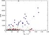 |
Fig. 1 Kepler signal-to-noise ratios (SNR) of short cadence planetary candidates as of 2012/02/27, versus number of transit data points per day (Np). Large markers indicate our target selection. Diamonds: high signal-to-noise sample (SNR ≥ 1000), big circles: sample with high impact parameters b ≥ 0.8 (SNR ≥ 150). |
Our high signal-to-noise target sample ordered by increasing Teff.
2.1.2. Targets with a high impact parameter
Measurements of LDCs strongly depend on the spatial information contained in the transit light curve. In the case of highly inclined transiting systems, synonymous with a large impact parameter, the planet crosses only a limited part of the stellar surface at the limb and the transit does not contain information on the brightness distribution at the disk center. The impact parameter b = (a/RS)cosi characterizes the path of the transit across the stellar disk. It depends on the semimajor axis a, normalized by the stellar radius RS, and the inclination angle i. An impact parameter of b = 0 corresponds to an inclination angle of 90°, i.e., a transit passing across the center of the disk, for b = 1, the center of the planet touches the stellar limb at transit center.
Howarth (2011b) simulated the effect of an increasing impact parameter on measured LDCs. He showed for different passbands that the measured LDCs show a systematic deviation from the model prediction. This means that a large impact parameter must be accounted for when fitting transit light curves and interpreting the results; most likely the LDCs of such systems will show much larger uncertainties even for very high SNR because the brightness distribution from the center to the limb is not covered by the data.
Following the work of Howarth (2011b) and studies made by our group for TrES-2 (Schröter et al. 2012), we also investigate systems with high impact parameters. Since TrES-2 is the only system in our high signal-to-noise sample with an impact parameter larger than 0.8, we decreased our SNR threshold from 1000 to 150 and selected all objects with an impact parameter b ≥ 0.8 from the KPCL. This leads to 13 additional systems. One object of this sample turned out to be a highly active binary system and was rejected from the list, leaving the high impact parameter sample with 12 members listed in Table 2.
2.2. Light curve normalization
The Kepler data show irregular variability caused by instrumental
effects and residuals of the reduction process including variations between different
Kepler quarters. Furthermore, some objects show intrinsic variability,
e.g. caused by starspots. Hence every transit light curve requires an individual
normalization which we perform by fitting a second order polynomial to the surrounding
out-of transit measurements. A simple linear fit is insufficient to properly remove
stellar or instrumental variations while higher orders turned out to result in instable
fits. We chose a duration of Δtconti = 4.5 h for the
off-transit parts which leads to ≈540 data points used for the normalization of each
transit. Equation (2) yields the lower and
upper boundary times of the normalization interval calculated relative to the
nth transit center
tc,n. We used the time
of the first recorded transit center t0 (BJD-2 454 900) and
the orbital period Porb given in the planetary candidates list
to determine the transit center times tc,n:
 To
account for inaccurate transit durations and orbital periods possibly contained in the
planetary candidates list, we adopted a tolerance ttol of 0.5
h, which results in a buffer of about 30 data points before the start of the transit
t1 = tc,n − tdur/2
and after its end
t4 = tc,n + tdur/2,
respectively. Both off-transit parts around a transit had to contain at least four data
points each, otherwise the transit was discarded. The total number
Ntotal of accepted transit light curves is listed in Table
B.1.
To
account for inaccurate transit durations and orbital periods possibly contained in the
planetary candidates list, we adopted a tolerance ttol of 0.5
h, which results in a buffer of about 30 data points before the start of the transit
t1 = tc,n − tdur/2
and after its end
t4 = tc,n + tdur/2,
respectively. Both off-transit parts around a transit had to contain at least four data
points each, otherwise the transit was discarded. The total number
Ntotal of accepted transit light curves is listed in Table
B.1.
Even after removing the data points flagged by the pipeline, a few outlying data points remain that cannot be attributed to noise and should not be taken into account for the normalization process. To identify such outliers we determined the median absolute deviation (MAD) within the selected continuum parts and set 0.6745-1MAD as 1σ error (Hampel 1974), which is a robust estimator of the standard deviation of normally distributed data in the presence of outliers; all data points 3σ away from the median of the continuum flux were filtered out.
All transit light curves were normalized by dividing them by a second order polynomial
according to  (3)The coefficients
a, b, and c were determined using a
downhill simplex algorithm on the intervals
[tconti, −,t1 − ttol]
and
[t4 + ttol,tconti, +]
minimizing χ2.
(3)The coefficients
a, b, and c were determined using a
downhill simplex algorithm on the intervals
[tconti, −,t1 − ttol]
and
[t4 + ttol,tconti, +]
minimizing χ2.
2.3. Assessment of transit data quality
In this section, we revisit the light curve normalization and analyze white and red noise in our transit light curves.
2.3.1. Refining the normalization
To search for poorly normalized transit light curves, we developed a filter algorithm which applies three linear fits to the normalized continuum. The first fit includes the whole 9 h of continuum selected for the normalization. The absolute value of the resulting gradient had to be lower than 1.5 × 10⁻⁷ d-1. Transits with higher values were discarded. For the remaining transits the left and right continuum parts were fitted separately. We set a gradient threshold of 1.5 × 10⁻³ d-1 which must not be exceeded by the fits. The threshold values were determined by eye after the inspection of normalized transit light curves; transits showing higher values displayed significant inconsistencies in their normalization.
In addition to this automatic method, it was necessary to discard transits manually, such as in the case where the transits are well normalized but distorted by starspots (HAT-P-11b) or where individual transit light curves show a much larger dispersion of data points than the majority of the other transits. The transit light curves rejected by these two methods are listed in Table B.1. The remaining number of transits used in our analysis is given by Ntransit in Tables 1 and 2.
2.3.2. Outlier removal and signal to noise
Outlier removal inside transit light curves is difficult if the real transit depth and shape are unknown. To remove prominent outliers, we used a sliding median filter of window size 10 min and rejected all points more than 4σ away.
The transit quality was measured by calculating the mean SNR per transit (δ/N) for each object in our sample. We determine the difference between the continuum level (=1) and the median flux value at transit center ℱmin determined in a 10 minutes interval around the transit center; this difference was defined to be our transit depth δ and the signal of the planet. We prefer this definition of the transit depth because it does not depend on the transit model. One could also use the radius ratio p resulting from a model fit as an estimator for the transit depth; however, this fit parameter would be correlated to other parameters, especially the LDCs. The noise value was calculated using 0.6745-1MAD in the corresponding continuum levels. The resulting mean signal-to-noise values are listed in Tables 1 and 2. We emphasize that these δ/N values are not to be confused with the SNR which is used to estimate the photometric quality of a data set (see Fig. 1). The δ/N estimates how much stronger the transit signal is than the photometric noise; for all objects in our samples δ/N is much smaller than the SNR values given in the KPCL.
2.3.3. Correlated noise analysis
Parameter estimates based on transit light curve modeling can be severely impeded by red (i.e., correlated) noise, whose sources are manifold including unaccounted for stellar variability and instrumental effects. However, the latter are likely small on transit timescales in the Kepler data. Kipping & Bakos (2011b) thoroughly study red noise in the Kepler light-curve of TrES-2 and find “no strong evidence for correlated noise”.
To check whether our transit light curves are affected by red noise, we follow the approach of Pont et al. (2006), which is based on a comparison of unbinned and binned residuals (see Carter & Winn 2009, Eq. (36)). In this approach red noise, if present, is accounted for in a conventional white-noise analysis by multiplying the measurement errors with a correction factor β.
Our analysis shows that the assumption of uncorrelated noise is justified in 32 of our 38 sample stars. In the remaining six objects we find red noise and correct the error estimates. They are discussed in Sect. 4.
3. Determination of transit parameters
3.1. Analytic transit model
When fitting transit data one has to determine at least five parameters: the center time
of the first observed transit t0, the orbital period
Porb, the ratio of the stellar and planetary radii
p, the inclination angle i, and the semimajor axis
a/RS. Fitting the
stellar limb darkening requires additional fit parameters depending on the adopted
limb-darkening law. Here, we choose the quadratic limb-darkening law
 (4)introducing two
additional parameters u1 and u2.
The variable μ is defined as cosθ where
θ is the angle between the line of sight and the inward surface normal
pointing to the occulted surface area. Hence, I(1) is the intensity at
the disk center where θ = 0°. To model each transit light curve with the
given parameters, we used the FORTRAN routine occultquad4 developed and provided by Mandel & Agol (2002), which generates a semi-analytical transit
model. We assumed circular orbits (e = 0) for all objects in our
selection.
(4)introducing two
additional parameters u1 and u2.
The variable μ is defined as cosθ where
θ is the angle between the line of sight and the inward surface normal
pointing to the occulted surface area. Hence, I(1) is the intensity at
the disk center where θ = 0°. To model each transit light curve with the
given parameters, we used the FORTRAN routine occultquad4 developed and provided by Mandel & Agol (2002), which generates a semi-analytical transit
model. We assumed circular orbits (e = 0) for all objects in our
selection.
3.2. Transit timing and parameter determination
A precise knowledge of the orbital period Porb and time of the transit center t0 is essential in the fitting process. Clearly, inaccurate values of Porb and t0 make a correct determination of the remaining transit parameters impossible. Hence, it is essential to determine Porb and t0 as accurately as possible.
As a first step we used the transit model introduced in Sect. 3.1 to fit these two parameters for each object using a downhill simplex algorithm, keeping all other parameters fixed to the values given in KPCL. The initial values for Porb and t0 were also taken from that list. The results of this fitting method were used as initial values for an MCMC sampling algorithm (Sect. 3.3).
After determining Porb and t0, we fitted the remaining parameters: the ratio of the star-planet radii p, the inclination angle i, the semi major axis a, and the quadratic LDCs u1 and u2. Again we started with a downhill simplex algorithm with initial parameter values taken from KPCL on the MAST website; afterward, we used these fit results as initial values for our MCMC sampling described in the following. We neither bin nor phase-fold the transit light curves during the fitting process.
3.3. MCMC modeling
We used a Markov chain Monte Carlo (MCMC) approach to sample from the posterior distribution of the parameters using 106 iterations of the sampler and discarding a burn-in of 40 000 iterations. The mean values of the parameter traces were then interpreted as the most probable parameters. We used the 68.3% highest probability density intervals (HPD) as our error estimate. For those parameters which require error propagation, such as the impact parameter b, we applied the corresponding equation to the MCMC parameter traces; then the HPD of the parameter can be determined from that new distribution.
The computation time for our 106 iterations per object was up to 15 h, depending mainly on the amount of transit light curves. All MCMC calculations make extensive use of routines of PyAstronomy5, a collection of Python routines providing an interface to fitting and sampling algorithms of the PyMC (Patil et al. 2010) and SciPy (Jones et al. 2001) packages.
4. Objects requiring special consideration
Some objects in our sample require special treatment, due to instrumental or other peculiarities such as red noise. Their analysis is detailed below.
4.1. HAT-P-11 (KIC 10748390)
HAT-P-11b (KIC 10748390), first reported on by Bakos et al. (2010), shows some transit light curves which cannot be properly normalized using Eq. (3). This is due to the fact that the continuum flux seems to be biased by an additive offset, which differs between the affected transits. The additive term influences the relative transit depth, in particular, higher absolute flux levels lead to a lower value of 1−ℱmin.
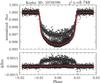 |
Fig. 2 Normalized and phase-folded transit light curve of HAT-P-11b. The manually deleted transit light curves are included, clearly visible above our best-fit model shown in red. This model only uses 18 out of 95 transits (see Table B.1). |
The affected transits can be identified in Fig. 2 by a systematic deviation from the transit mean greatly exceeding the statistical noise. Additionally, HAT-P-11A shows starspots transited by the planet resulting in bumps distorting at least some transit profiles (Sanchis-Ojeda & Winn 2011).
In our analysis, we removed all transits that show detectable starspot crossings or cannot be normalized appropriately due to the offset problem (see Table B.1). Nonetheless, we find a red-noise contribution in the residuals of the remaining transit light curves, leading to a correction factor of β ≈ 1.49 (see Sect. 2.3). We ascribe the red noise in this case to unresolved starspot signatures.
4.2. KIC 8845026
The light curve of KIC 8845026 is modulated with a peak-to-peak amplitude of ≈0.2% and a period of roughly 4 days, likely due to rotational modulation. Due to the long orbital period of ≈66.5 d, our data contains only five transits. The transit duration amounts to nearly 20 h, which is comparable to the observed variability timescales and affects the transit profile. Thus, we find that different transits cannot be consistently normalized and show different depths after normalization. We decided to limit our analysis to the transit light curve showing the lowest red-noise contribution (β = 1.36).
4.3. HAT-P-7b and KIC 9631995
Figures 3 and 4 show the normalized and phase-folded transit light curves of KIC 10666592 (HAT-P-7b, Pál et al. 2008) and KIC 9631995. Our filter algorithm introduced in Sect. 2.3 found all transits to be well normalized for both objects. Also our outlier removal showed no inconsistencies for the transits of these data sets.
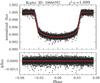 |
Fig. 3 Normalized and phase-folded transit light curve of HAT-P-7b. Ten manually deleted transit light curves are included. |
However, some transit light curves had to be removed manually because they show outliers significantly below the average light curve and a stronger dispersion probably caused by instrumental effects or the data reduction. While KIC 9631995 shows white noise in the remaining transit light curves, we find red noise in HAT-P-7b and corrected for it by using β = 1.60.
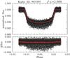 |
Fig. 4 Normalized and phase-folded transit light curve of KIC 9631995. Eight manually deleted transit light curves are included in this figure. |
4.4. Kepler-17b and KIC 3861595
Kepler-17b (KIC 10619192) shows red noise in the residuals of our transit modeling (see Fig. B.2, last row). Its light curve has previously been discussed by Désert et al. (2011), who report rotational variability with a peak-to-peak amplitude on the order of 3% and prominent starspot crossing events. Therefore, the correlated noise is likely attributable to starspots. Our analysis yields a correction factor of β ≈ 1.65 .
The situation is similar for KIC 3861595, a member of our high impact parameter sample, in the light curve of which we also detect red noise, leading to β ≈ 1.94. Its light curve shows potential rotational modulation with a peak-to-peak amplitude of about half a percent. Consequently, the red noise may be introduced by starspot crossings for this object.
4.5. Kepler-13
Kepler-13 (KIC 9941662) transits the hottest star of our sample. Its light curve has been studied by Barnes et al. (2011), who report on an asymmetry in the model residuals which they attribute to gravitational darkening. The same asymmetry is seen in our analysis, resulting in a red noise detection (β ≈ 1.40). Furthermore, the Kepler aperture contains a second star contributing about 45% of the observed flux (Szabó et al. 2011), which we take into account in our modeling. We argue that the asymmetry introduced by gravitational darkening is on the order of 10-4 and does not severely affect our analysis. Furthermore, we verified that the limb-darkening coefficients do only slightly depend on the third light contribution (in the order of ≈± 0.01), which is relatively well known. Therefore, we retain Kepler-13 in our sample.
5. Results and discussion
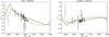 |
Fig. 5 Quadratic LDCs determined by MCMC for our high signal-to-noise target sample (see Table 1). For comparison, the graphs show model predictions based on PHOENIX (solid) and ATLAS (dashed) atmospheric models, taken from Claret & Bloemen (2011). The dotted lines show Claret and Bloemen’s LDCs determined for the same atmospheres by different methods (see Sect. 5.1). The diamond symbol indicates TrES-2, which has the highest impact parameter of this sample (b = 0.845). Triangles mark conspicuous objects, discussed in Sect. 5.3. |
In Table 3 we show the results of our transit modeling, which we use in the following analysis. We compare these results to the quadratic LDCs predicted by Claret & Bloemen (2011) for Kepler’s spectral response function. Table 3 shows all seven determined transit parameters for all objects in our sample. In Sect. 5.2 we provide a detailed discussion on the fitted LDCs of our high signal-to-noise sample.
5.1. Theoretical LDCs
The key aim of our study is the comparison of our LD measurements with model LDCs determined from stellar atmosphere models. To this end we use the LDCs of Claret & Bloemen (2011). They are given in tables6 on which we linearly interpolate. The coefficients are determined from 1D-plane-parallel PHOENIX and ATLAS model atmospheres using two different methods (Claret 2000, Chap. 2.2): a flux-conserving fit method and a simple least squares fit to the theoretical stellar intensity distribution. These two fit methods lead to slightly different values of u1 and u2.
In Figs. 5 and 7 we show theoretical LDCs as a function of effective temperature derived from stellar atmosphere models with surface gravity log (g) = 4.5, metallicity [M/H] = 0.0, and micro-turbulent velocity ξ = 2.0 km s-1, in comparison to our measured LDCs. LDCs assigned as dotted lines come from the flux conserving fit method.
Apparently the LDCs do not only depend on the effective temperature but also on the other stellar parameters. The parameters used to derive the theoretical LDCs presented in Figs. 5 and 7 may not be appropriate for all stars in our sample. To estimate the influence of surface gravity and metallicity on the LDCs, we investigated different parameter sets and present the results in Figs. A.1 and A.2. We conclude that changes in metallicity or surface gravity in the ranges reasonable for our sample, have only a small effect on the predicted quadratic LDCs for stars in the temperature range of 4600 to 7800 K. Objects colder than Teff ≲ 4600 K show a stronger dependence on these parameters. This is important for the analysis of the coldest object in our selection. The theoretical LDCs determined from PHOENIX model atmospheres for each object, adopting the surface gravities from the KPCL, are listed in Table 3.
5.2. High signal-to-noise sample
Looking at the left panel of Fig. 5, we identify four objects that lie significantly below the theoretical predictions and have large error bars. Three are marked with triangles, TrES-2 is specifically marked with a diamond symbol. They have effective temperatures of 3948 K, 5814 K (TrES-2), 5912 K, and 6025 K, listed in Table 1. The right panel of Fig. 5 shows the measured values of u2. Again the same four objects lie among those with the largest errors, we discuss them in detail in Sect. 5.3.
Out of 26 objects 21 show a good agreement, within their errors, with at least one of the model predictions of u1. In contrast, the theoretical values of u2 tend to be systematically too high in the temperature range between 5300 to 6500 K. Subtracting an offset of ≈0.05 leads to a significantly better agreement between the measurements and the predictions of u2. Most of the fitted LDCs are consistent with those determined from one of the two model atmospheres, whereas the PHOENIX predictions seem to be the better choice for u2 in the regime of Teff > 4600 K.
Most objects of our sample have effective temperatures between 5000 K and 6400 K, which corresponds to F-, G-, and K-stars. Only a few exceptions, such as the ones at ≈4000 K and ≈8900 K, are lying outside of this conglomerate. Thus, our analysis of LDCs will be most reliable in the regime of solar-like stars, where we have a significant number of objects; the two exceptions can serve as indicators for the reliability of theoretical LDCs in more extreme regimes.
For a better illustration of the agreement between measured and theoretical LDCs, we present the sum of the quadratic LDCs u1 + u2 in Fig. 6 in the temperature range of 5300 K to 6500 K in which most objects of our sample are located. In this case the theoretical predictions from PHOENIX and ATLAS models are virtually identical. If the observed u1 and u2 are independently consistent with the models, their sum has to agree with the theory as well. However, out of 20 objects only four lie on the model predictions within their errors while 16 objects show significantly lower values. The median value of the residuals is Δu1 + u2 = −0.07 ± 0.01. As already seen for the values of u2, there appears to be an offset between measurements and predictions, which is, at least in the case of PHOENIX models, largely caused by a systematic shift of the u2 values. This indicates that the coefficient of the quadratic term in the LD law is slightly overestimated by theory, as already suggested by the right panel of Fig. 5.
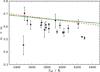 |
Fig. 6 Sum of the linear and quadratic limb-darkening coefficients for objects with an impact parameter b < 0.8 of our high signal-to-noise sample in comparison to the summed model predictions (solid: PHOENIX, dashed: ATLAS). |
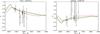 |
Fig. 7 Same as Fig. 5 for objects with impact parameters larger than 0.8 as given in the Kepler planetary candidates list (i.e. our high-impact-parameter sample, see Table 2). According to our transit modeling only objects marked with diamonds truly have b ≥ 0.8 while we found b < 0.8 for the objects indicated by dots. |
5.3. Outlier objects
Figure 5 contains several points with relatively large errors. In this section we discuss the four objects with the highest uncertainties in both LDCs u1 and u2, which are also the objects with the largest deviation from the predictions. In the left panel of Fig. 5, these objects lie clearly below the LDC predictions and are marked with triangles and a diamond symbol. Below, we discuss them in order of increasing effective temperature.
According to the KPCL, the first “outlier”, KIC 5794240, has an effective temperature of 3948 K and a surface gravity of log (g) = 4.72. Most objects in the KPCL have Teff credible to within ± 200 K and log (g) with errors of about ± 0.4 (Brown et al. 2011). As already stated in Sect. 5.1, the theoretical predictions in Fig. 5 are based on atmosphere models with log (g) = 4.5. Although this is consistent with the estimated error of the measured log (g), the influence of log (g) on the LDCs becomes important for Teff ≲ 4600 K (see Fig. A.1), which is the case for KIC 5794240. In this temperature range an increase in log (g) leads to significantly lower values of u1. An agreement with the measurement is reached for a log (g) of about 5.0 using ATLAS model atmospheres. Surface gravities of 5.0 or higher are not uncommon for M5-dwarfs (see PASTEL catalog, Soubiran et al. 2010) and are fully consistent with the above error estimate.
The metallicity Z = [M/H] also has a significant influence on u1 and u2 in this temperature region (see Fig. A.2). Potentially, the Z value of KIC 5794240 (=0.2) is poorly determined since most metallicities of the KPCL are highly uncertain (Brown et al. 2011). A lower metallicity of, e.g., [M/H] = −0.3, leads to theoretical LDCs consistent with the observation. In the light of our analysis, a subsolar metallicity of KIC 5794240 seems to be more reasonable than its super-solar metallicity stated in the Kepler Input Catalog (Brown et al. 2011).
Finally, the light curve of KIC 5794240 indicates substantial stellar activity. The visible photometric variations suggest rotational modulation due to starspots. It is reasonable to expect that some of the spots are occulted by the planet when crossing the disk, leading to deformations of the transit profile (see, e.g., Huber et al. 2010). The detailed investigation of how starspots influence the determination of LDCs is beyond the scope of this work, however, the strong temperature dependence of LD suggests a non-negligible effect for substantially spotted stars. Thus, the inconsistency with the model and the large uncertainties of the measured LDCs of KIC 5794240 could also reflect the effects of stellar activity on its light curve.
The diamond symbol in Fig. 5 marks the second “outlier”, TrES-2, an intensively studied exoplanetary system. It has the highest SNR of all planet host stars in the Kepler sample. Nonetheless, the uncertainties of the LDCs are large (σ ≈ ± 0.2) compared to other objects with lower SNRs, and the determined LDCs are inconsistent with the model predictions. However, TrES-2 has a rather large impact parameter of b = 0.85 and, therefore a nearly grazing transit, which is the reason for the big uncertainties of the measured LDCs and the large deviation from theory. We investigate this behavior in Sect. 5.4 in detail.
The last two objects of our outlier sample, KIC 7877496 and KIC 6922244 (Kepler-8b), show the same behavior as TrES-2. The number of available and fitted transit light curves for both objects are comparable to TrES-2. These systems also have high impact parameters of b ≈ 0.8 (see Table 3) which causes the strong deviation from the theoretical LDCs of these objects and big uncertainties.
5.4. Objects with high impact parameters
As discussed in the previous section, TrES-2, Kepler-8, and KIC 7877496 show a common behavior due to their large impact parameters: they exhibit large uncertainties in their fitted LDCs and lie below the theoretical models for u1 and above for u2. A similar behavior has already been found by Howarth (2011b) who simulated the influence of a high impact parameter on the determination of quadratic LDCs.
To further investigate this behavior, we analyze a sample of twelve objects with impact parameters larger than 0.8 as given in the KPCL (see also Sect. 2.1.2 and Table 2). Our measured quadratic LDCs are presented in Fig. 7 and compared to the same theoretical values as in Fig. 5.
According to our transit modeling, 5 of the 12 objects actually have b < 0.8 (see Table 3). For those systems, the impact parameters of the KPCL appear to be incorrect. These objects, marked as dots in the figure, agree well with the model predictions. The others have impact parameters of b > 0.8 (diamond symbols) and significantly deviate from theory in the same manner as those discussed in Sect. 5.3. Again we can see that u1 is systematically underestimated while the values of u2 lie above the prediction.
Figure 8 illustrates the increase in the deviation between measurements and theory with increasing impact parameter. It shows the sum of the squared differences between the measured LDCs and the PHOENIX model predictions denoted by m1 and m2 as a function of b for all objects of our study. The differences between measurements and theory are small for impact parameters up to about 0.8. However, for objects with impact parameters b ≳ 0.8 the deviations from the model predictions as well as the measurement errors increase significantly. Hence, for impact parameters exceeding about 0.8 a reliable determination of LDCs from a transit light curve fit becomes intricate.
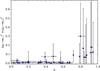 |
Fig. 8 Summed quadratic deviation of measured LD coefficients from those calculated from PHOENIX models versus impact parameter. |
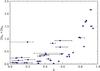 |
Fig. 9 Summed width of the 68.3% HPD intervals for u1 and u2 versus the impact parameter b as determined by MCMC. See text for details. |
A similar behavior as found in Fig. 8 can also be seen if only the measurement errors are considered – independently of the atmospheric model predictions (m1 and m2). This is shown in Fig. 9, where we plot the summed widths of the 68.3% credibility intervals for u1 and u2, against our measured system impact parameters. For b around 0.8 and larger, a considerable increase in the resulting uncertainties is detectable. It seems that there is some transition at b ≈ 0.8 where the determination of LDCs becomes much more difficult. We discuss this behavior in more detail in Sect. 5.6.
Setting the LDCs as free fit parameters influences the determination of the remaining transit parameters due to strong correlations. This applies especially to the case of large b, as a consequence it is highly inadvisable to fit the LDCs in systems with high impact parameters.
5.5. Deviations between measured and predicted LDCs and their influence on transit modeling
Figure 5 illustrates the key result of our study, namely the relation between the measured and predicted limb-darkening coefficients. Considering the difference between the PHOENIX and ATLAS model predictions as the systematic uncertainty of the theoretical LDCs, we find that our values derived for the linear coefficient u1 are fully consistent with the models within these uncertainties. Thus, the predictions of u1 span an allowed band of coefficients confirmed by our measurements. On the other hand, both ATLAS and PHOENIX tend to overestimate the quadratic LDC u2 when compared to our measurements.
The typical deviation between our measurements and the model predictions amounts to about 0.05 both in u1 and u2. We estimated the influence of such deviations in the LDCs on the planetary parameters derived by transit modeling: as outlined in Sect. B.5, we derive a Gaussian approximation for the posterior probability distribution, modify the limb-darkening coefficients based on the alleged deviations,
Assuming that the discrepancy in Δu1 + u2 (cf., Sect. 5.2) is exclusively caused by a deviation in u2, we use this approach to derive average relative changes of Δa/a = 1.3%, Δi/i = 0.4%, and Δp/p = −0.6%. Comparing our LD measurements to the PHOENIX predictions, we find average offsets of Δu1 = −0.05 ± 0.01 and Δu2 = −0.03 ± 0.01. These translate into relative parameter changes of Δa/a = 1.6%, Δi/i = 0.5% and Δp/p = −0.7%. Hence, the deviations in the LDC found in our study result in moderate errors on the order of one percent in relative accuracy with the semimajor axis responding most sensitively to changes in the LDCs.
5.6. Correlation between the quadratic LDCs and their systematic uncertainties
In the previous sections, we have demonstrated that the quadratic LDCs u1 and u2 can be determined with small measurement errors and that the result is in reasonable agreement with theory for small and moderate impact parameters. Our MCMC analysis shows that both LDCs are strongly correlated. If we take a look at the combination uC = u1 + u2, we see that this parameter has a substantially lower error than the two coefficients alone. It seems to be an inherent property of the quadratic LD model that the combination uC is always much better constrained than the individual LDCs.
This is even the case for systems with b ≳ 0.8. Here, u1 and u2 show large errors and deviations from theory, but their sum uC shows significantly smaller errors and is still consistent with the model predictions. The sum of u1 and u2 is presented in Fig. 10 along with the theoretical LDCs; the deviations from the theory are significantly smaller than in Fig. 7 for the individual coefficients.
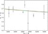 |
Fig. 10 Sum of the linear and quadratic coefficients uC = u1 + u2 for objects with an impact parameter b > 0.8 in comparison to the summed model predictions (solid: PHOENIX, dashed: ATLAS). |
As already pointed out by Schröter et al. (2012,
Eq. (1)), the quadratic LD law can be approximated by a constant function
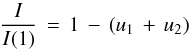 (5)under the assumption
μ ≪ 1, i.e. systems with very high impact parameters7. Physically, this means that one only measures the brightness at the
stellar limb, which does not show a functional relation to μ anymore but
is only a constant difference to the central brightness I(1). In such
systems a transit fit would only be sensitive to the sum of the LDCs.
(5)under the assumption
μ ≪ 1, i.e. systems with very high impact parameters7. Physically, this means that one only measures the brightness at the
stellar limb, which does not show a functional relation to μ anymore but
is only a constant difference to the central brightness I(1). In such
systems a transit fit would only be sensitive to the sum of the LDCs.
Although this certainly is part of the explanation, our analysis shows that the situation is more complex. We present an analytical approximation for the errors of the LDCs in Appendix B. We find that uC is always better constrained than the individual coefficients independent of the impact parameter, which is a general characteristic of the quadratic LD law; this result is visualized in Fig. 11. Only for high values of b we find that the individual LDCs are virtually unconstrained by transit modeling.
The analytical solution given in Appendix B allows investigating the errors and the correlation of u1 and u2. We compare our results to simulations using a transit model with fixed planetary parameters; only the impact parameter is varied between 0 and 1. Our results are presented in Figs. 11 and B.1. The behavior of the simulations is reproduced by theory: the measurement errors of u1 and u2 are smallest for low impact parameters and dramatically increase for b ≳ 0.8. This resembles our observations. Interestingly, the error does not increase monotonically, but decreases slightly after a local maximum at about b ≈ 0.5 before it rises steeply again. This means that LDCs are slightly better constrained for values of ≈0.8 than for values of ≈0.5.
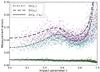 |
Fig. 11 Simulated measurement errors (dots) for the individual LDCs u1 (cyan), u2 (purple) and for the sum u1 + u2 (green) as determined by transit modeling. For the simulation we used fixed parameters only the impact parameter was varied between 0 and 1. The overplotted lines show our analytical solutions (see Appendix B for details). |
Our simulations and our analytical treatment show the same behavior of the correlation of u1 and u2 as a function of the impact parameter. Both coefficients are highly anti-correlated even for small impact parameters. Their correlation coefficient decreases to −1 for b ≈ 1, where their individual errors increase rapidly. This is the explanation for the behavior visible in Fig. 7, where u1 and u2 values for high impact parameters have not only much larger errors but also lie systematically below the prediction for u1 and above it for u2. Their strong anti-correlation is well visible in this regime and a shift of u1 in one direction is compensated by a shift of u2 to the other direction.
6. Summary and conclusions
The measurement of stellar limb darkening (LD) is notoriously difficult, because almost no stellar disk can be spatially resolved. A new and promising opportunity to measure stellar LD is the use of high-precision transit light curves. Here, the planet serves as a scanner of the stellar brightness distribution during its disk passage.
From the list of Kepler planetary candidates, we construct two samples: (1) a high signal-to-noise sample with 26 objects and (2) a sample comprising 12 high impact-parameter systems (b ≥ 0.8). However, according to our transit modeling, only seven of the alleged 12 planetary systems in our high impact-parameter sample truly deserve this designation. The majority of our sample objects are late F-, G-, and early K-type main-sequence stars spanning an effect temperature range from 4600 K to 6400 K.
We measure the quadratic LDCs u1 and u2 using a Bayesian MCMC approach and compare them to theoretical predictions based on PHOENIX and ATLAS stellar atmosphere models. Our results show that reliable limb-darkening coefficients (LDCs) can be determined using the most accurate transit observations of the Kepler space telescope.
The differences between the PHOENIX and ATLAS model predictions are as large as 0.1 in both LDCs in the effective-temperature regime under consideration. For the linear coefficient, u1, our measurements are mainly distributed between the PHOENIX and ATLAS model predictions. Interpreting the deviation between the models as systematic uncertainty, we argue that our u1 measurements agree with the theoretical predictions. In fact, they are equally consistent with either.
For the quadratic coefficient, u2, our measurements do show a
systematic offset: most of our measurements lie below the predictions of both atmospheric
models. However, on average, u2 deviated by −0.1 from the ATLAS
and by −0.03 from the PHOENIX models. This yields  making the PHOENIX models a better
fit.
making the PHOENIX models a better
fit.
Nonetheless, our measurements show a slightly weaker limb darkening than either model. Interestingly, the 3D-hydrodynamic atmospheric models presented by Asplund et al. (2009) predict a LD weaker by an amount comparable to our findings (see also Hayek et al. 2012; Trampedach et al. 2013). However, this prediction is not universally shared among hydrodynamic 3D models (Hauschildt & Baron 2010).
An important factor for the measurement of LDCs is the impact parameter of a system. All our measurements for objects with high impact parameters show deviations from the theoretical LDCs. This has already been suggested by simulations (Howarth 2011b). According to our Figs. 8 and 9, we find that impact parameters in the range of b ≳ 0.8 are critical in the sense that for those the uncertainties in u1 and u2 increase drastically. Only their sum u1 + u2 can still be reliably determined. This behavior can be reproduced in our analytical approximation of the transit modeling with quadratic LDCs.
We note that the surface gravity log (g) and metallicity Z significantly influence the theoretical LDCs only for effective temperatures below 4500 K and in a narrow region above 7500 K. For stars outside these temperature ranges, i.e., all but two of our sample stars, the theoretical LDCs can be used without introducing a severe error resulting from inaccurately known log (g) and Z values.
Although we do find a deviation between theory and measurements, we estimate that the error propagated into the remaining fit parameters by fixing the LDCs to theoretical values amounts to roughly one percent for the semimajor axis, inclination, and planetary radius determined by light curve modeling and thus should be negligible for many applications.
Therefore, we conclude that the quadratic LDCs can be fixed to theoretical values (e.g., tabulated by Claret & Bloemen 2011) in the process of transit analysis. For high impact parameter systems (b ≳ 0.8) or observations with significantly lower SNR than the Kepler data, we even recommend to fix the LDCs to model predictions, since the LDCs remain badly constrained by transit modeling in both cases.
Online material
Transit modeling results.
Appendix A: Influence of stellar parameters on the theoretical LDCs
Stellar limb darkening depends on fundamental stellar parameters as, e.g., the effective temperature Teff and the surface gravity log (g). For a plausible comparison between theoretically determined and measured LDCs it is necessary to know the correct stellar parameters for each studied object. While the Kepler Input Catalog (KIC, Brown et al. 2011) already provides Teff, log (g), and metallicities Z determined using ground-based photometric observations, the Kepler planetary candidates list (KPCL) offers values determined using other methods, e.g., spectroscopic follow up observations. The fundamental parameters of the Kepler stars are determined by four different methods as described by Batalha et al. (2013). The method actually applied to the object at hand is indicated by the fTeff-flag given in the KPCL. They can be divided into two groups: The first group (0, 1) uses photometric data and, e.g., matches the KIC parameters to Yonsei-Yale stellar evolution models (Demarque et al. 2004). The second group (2, 3) uses spectroscopic follow-up observations determining the parameters using spectroscopy made easy SME (fTeff = 3, Valenti & Piskunov 1996) or the stellar parameter classification tool SPC (fTeff = 2, Buchhave et al. 2012), see KOI-list8 for further details. Naturally, the stellar parameters derived by spectroscopic methods are more reliable. None of our target stars has an fTeff-flag equal to 0, 14 have fTeff = 1, and the majority has fTeff of equal to 2 or 3 (see Table A.1). In the case of photometrically determined parameters (fTeff = 1) one has to keep in mind that the stellar parameters, especially the metallicities, have the highest uncertainties. In this case, the typical errors of Teff and log (g) are about ± 200 K and 0.4, whereas Z is basically undetermined (Brown et al. 2011). The uncertainties decrease, especially for log (g) and Z, for parameters derived by spectroscopic methods.
The influence of log (g), Z, and the micro-turbulent velocity ξ on the LDCs varies with effective temperature. This has already been theoretically studied, e.g. by Claret (2000) for a four parameter nonlinear LD law. We discuss the influence for the parameter range relevant for our analysis by using Claret & Bloemen (2011) LDCs (for ATLAS models). Since the quadratic coefficient u2 shows virtually the same behavior as u1, we concentrate on u1. In Fig. A.1 we show the effect of log (g) on u1 by calculating the difference between u1 determined with log (g) = 4.5 and values of u1 for a slightly higher (4.8) and lower (4.3) surface gravity. For effective temperatures in the range from ≈4500 K to ≈7500 K, which covers the majority of stars in our sample, there is no significant influence of the surface gravity. However, especially for cooler stars (Teff ≲ 4500 K) the LD becomes sensitive to log (g).
fTeff-flags of our selection sorted by Teff, as given in the KPCL.
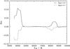 |
Fig. A.1 Influence of log (g) on the LDC u1. Shown is the difference between u1 determined with log (g) = 4.5 and values of u1 using a higher (4.8) and lower (4.3) surface gravity, over a wide temperature range (ATLAS models). |
Figure A.2 shows the result of a similar analysis, this time varying the stellar metallicity Z. Again the effect on the LDC is strongest for stars cooler than ≲4500 K, but there are already significant deviations in the range between 4500 K to ≈6500 K. A change in metallicity of ±0.5 in this temperature range results in a maximum Δu1 of ±0.05.
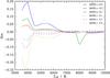 |
Fig. A.2 Influence of the stellar metallicity on u1. Differences between u1 determined with [M/H] = 0.0 and values of u1 using different metallicities are plotted against Teff (ATLAS models). |
The micro-turbulent velocity has only a rather weak influence on the LDCs. The difference Δu1 calculated between u1 determined for ξ = 0.1 km s-1 and ξ = 8.0 km s-1 never exceeds ± 0.015 and, thus, is negligible.
We conclude that metallicities and surface gravities do not have a crucial effect on predicted LDCs for stars in the temperature range of 4500 to 7500 K. We note that for most objects in the solar neighborhood the absolute value of Z is lower than 0.5 (Casagrande et al. 2011) and it is appropriate to assume that our ignorance of the metallicity of the Kepler planetary candidates does not introduce a significant bias for the determination of theoretical LDCs. The most important parameter is the effective temperature which is often quite reliably determined even when using only color indices.
Appendix B: Analytical approach to the limb-darkening fits
 |
Fig. B.1 Comparison of simulations (dots) and our analytical solutions (lines). Left and center: dependency of the measurement errors on the system impact parameter b. Right: correlation coefficients of the LDCs with increasing b. See Sect. B.4 for details. |
In the following we provide an analytical approach to the problem of fitting limb-darkening coefficients. Our treatment aims at a fundamental understanding of the accuracy and correlation of limb-darkening coefficients determined from transit fits.
To simulate the measurement errors, we carried out a Monte-Carlo simulation. In particular, we constructed transit light curves for a hypothetical planet with a period of Porb = 2.47 d, a semimajor axis of a = 8.4 stellar radii, and a small planet-to-star radii ratio of p = 10-3. The small planet size is important for our comparison of these simulations to our analytical results which are only valid for small p (≪1). We set the values of the quadratic limb darkening to u1 = 0.5 and u2 = 0.2. Using these parameters, we created simulated light curves with a δ/N of 60 (as defined in Sect. 2.3) and 85 equidistantly distributed photometric points during the transit. Although we kept the temporal cadence constant, we allowed the time axis to shift with respect to the transit center in consecutive runs to avoid systematics arising from an unrealistically symmetric simulation. We then proceeded to sample from the posterior probability distribution using an MCMC algorithm and the transit models provided by Mandel & Agol (2002) with the LDCs as only free parameters. The resulting Markov-chains allow credibility intervals for the LDCs and the correlation coefficient ϱ to be derived. Each point in Figs. 11 and B.1 represents an individual simulation.
Appendix B.1: Modeling the transit profile
In our approach, we consider the following simplified transit light curve model
![Mathematical equation: \appendix \setcounter{section}{2} \begin{equation} y(t_i) = 1 - \frac{ \left[ 1-u_1 \left( 1-\mu(t_i) \right) - u_2 \left( 1-\mu(t_i) \right)^2 \right] \, p^2 }{1-\frac{u_1}{3}-\frac{u_2}{6}} , \label{eq:Model} \end{equation}](/articles/aa/full_html/2013/12/aa22079-13/aa22079-13-eq481.png) (B.1)where
ti is the ith time of
measurement, μ = cos(θ) where θ is
the angle between the line of sight and the inward surface normal of the position on
the stellar surface occulted by the planet, p is the ratio of the
planetary and stellar radii, and u1 and
u2 are the linear and quadratic limb-darkening
coefficients. The model described by Eq. (B.1) considers the amount of light blocked due to the size of the planet but
it neglects all other geometrical effects caused by the extent of the planet. In
particular the planet passes only one μ −value per
time step, which is fully consistent with our chosen small planet approximation
(p ≪ 1). The numerator accounts for the light blocked by the
planetary disk, while the denominator ensures a renormalization of the entire
brightness.
(B.1)where
ti is the ith time of
measurement, μ = cos(θ) where θ is
the angle between the line of sight and the inward surface normal of the position on
the stellar surface occulted by the planet, p is the ratio of the
planetary and stellar radii, and u1 and
u2 are the linear and quadratic limb-darkening
coefficients. The model described by Eq. (B.1) considers the amount of light blocked due to the size of the planet but
it neglects all other geometrical effects caused by the extent of the planet. In
particular the planet passes only one μ −value per
time step, which is fully consistent with our chosen small planet approximation
(p ≪ 1). The numerator accounts for the light blocked by the
planetary disk, while the denominator ensures a renormalization of the entire
brightness.
Given a circular planetary orbit with a period Porb,
inclination i, and a semimajor axis a, in units of
stellar radii, μ(ti) is
given by ![Mathematical equation: \appendix \setcounter{section}{2} \begin{eqnarray} \label{eq:mu_complex} \mu(t_i) &=& \sqrt{1 - a^2 \left[ \cos^2(i)\cos^2(\omega t_i)+\sin^2(\omega t_i) \right]}\nonumber\\ &=& \sqrt{1 - z(t_i)^2} , \end{eqnarray}](/articles/aa/full_html/2013/12/aa22079-13/aa22079-13-eq487.png) (B.2)where
z(ti) denotes the
sky-projected distance between the centers of the planet and the star. For a large
semimajor axis we can approximate
μ(ti) by
(B.2)where
z(ti) denotes the
sky-projected distance between the centers of the planet and the star. For a large
semimajor axis we can approximate
μ(ti) by
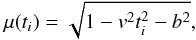 (B.3)where
 is the orbital velocity and
b = acos(i) is the impact
parameter, both in units of stellar radii.
is the orbital velocity and
b = acos(i) is the impact
parameter, both in units of stellar radii.
Appendix B.2: Expansion of χ2
Given a number of measurements, mi, with
measurement errors σ, the χ2-statistics
is defined as 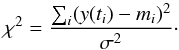 (B.4)This
expression can be expanded to second order with respect to the limb-darkening
coefficients u1 and u2:
(B.4)This
expression can be expanded to second order with respect to the limb-darkening
coefficients u1 and u2:
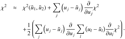 (B.5)Expanding
around the χ2-minimum,
(B.5)Expanding
around the χ2-minimum,
 ,
encountered for some combination of limb-darkening coefficients
,
encountered for some combination of limb-darkening coefficients
 and
and  ,
the χ2-increase, Δχ2, caused
by a deviation from the best-fit parameters reads
,
the χ2-increase, Δχ2, caused
by a deviation from the best-fit parameters reads 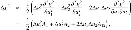 (B.6)where
the various A coefficients are abbreviations for the second
derivatives of χ2 and with
(B.6)where
the various A coefficients are abbreviations for the second
derivatives of χ2 and with
 and
and  .
.
Equation (B.6) describes an ellipse
with semimajor axis, aell, semiminor axis,
bell, and rotation angle α, which may
alternatively be written as 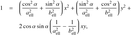 (B.7)when
we rotate the Cartesian coordinate system clockwise to achieve a counterclockwise
rotation of the ellipse. Comparing Eqs. (B.6) and (B.7), we determine
(B.7)when
we rotate the Cartesian coordinate system clockwise to achieve a counterclockwise
rotation of the ellipse. Comparing Eqs. (B.6) and (B.7), we determine
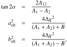 (B.8)where
B serves as an abbreviation for
(B.8)where
B serves as an abbreviation for
 .
To obtain the 68% confidence interval for two parameters of interest,
Δχ2 needs to be set to 2.3 or to 6.18 for 95% confidence
interval, respectively (Press et al. 2002).
.
To obtain the 68% confidence interval for two parameters of interest,
Δχ2 needs to be set to 2.3 or to 6.18 for 95% confidence
interval, respectively (Press et al. 2002).
Appendix B.3: The derivatives of χ2
The second derivative of χ2 with respect to the
limb-darkening coefficients can be written as 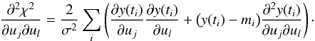 (B.9)The expressions for
the partial derivatives read
(B.9)The expressions for
the partial derivatives read
![Mathematical equation: \appendix \setcounter{section}{2} \begin{eqnarray} && \frac{\partial y}{\partial u_1} = 6\,{\frac {{p}^{2} \left( 4+{\it u_2}-6\,\mu-3\,{\it u_2}\,\mu+2\,{\it u_2}\,{\mu}^{2} \right) }{ \left( -6+2\,{\it u_1}+{\it u_2} \right) ^{2}}} \nonumber \\[3mm] && \frac{\partial y}{\partial u_2} = {\frac {-6\,{p}^{2} \left( 1-3\,\mu+2\,{\mu}^{2} \right) {\it u_1}-6\,{ p}^{2} \left( -5+12\,\mu-6\,{\mu}^{2} \right) }{ \left( -6+2\,{\it u_1} +{\it u_2} \right) ^{2}}} \nonumber \\[3mm] && \frac{\partial^2 y}{\partial u_1\partial u_1} = -24\,{\frac {{p}^{2} \left( 4+{\it u_2}-6\,\mu-3\,{\it u_2}\,\mu+2\,{ \it u_2}\,{\mu}^{2} \right) }{ \left( -6+2\,{\it u_1}+{\it u_2} \right) ^ {3}}}\ \nonumber \\[3mm] && \frac{\partial^2 y}{\partial u_2\partial u_2} = 12\,{\frac {{p}^{2} \left( -5+{\it u_1}+12\,\mu-3\,{\it u_1}\,\mu-6\,{ \mu}^{2}+2\,{\mu}^{2}{\it u_1} \right) }{ \left( -6+2\,{\it u_1}+{\it u_2 } \right) ^{3}}} \nonumber \\[3mm] && \frac{\partial^2 y}{\partial u_1\partial u_2} = -6\,{p}^{2}\left({\frac { \left( 14-2\,{\it u_1}+{\it u_2}-30\,\mu+6\,{\it u_1} \,\mu \right) } { \left( -6+2\,{\it u_1}+{\it u_2} \right) ^{3}}} \right. \nonumber \\[3mm] & & \qquad\qquad \left. +\frac{-3\,{\it u_2}\,\mu+12\,{\mu}^{2}-4\,{\mu}^{2}\it u_1+2\,{\it u_2} \,{\mu}^{2}}{ \left( -6+2\,{\it u_1}+{\it u_2} \right) ^{3}} \right) \cdot \end{eqnarray}](/articles/aa/full_html/2013/12/aa22079-13/aa22079-13-eq517.png) (B.10)These
derivatives can be evaluated for any combination of limb-darkening coefficients. The
orbit configuration and times of measurement are contained in μ
according to Eq. (B.3).
(B.10)These
derivatives can be evaluated for any combination of limb-darkening coefficients. The
orbit configuration and times of measurement are contained in μ
according to Eq. (B.3).
Especially the last term in Eq. (B.9)
is a nuisance, because it depends on the actual data set through
mi. As we, however, expand around the
χ2-minimum, the expectation value of this term equals
zero, because
(y(ti) − mi) σ-1
follows a standard normal distribution. The expectation value of the absolute value,
| ∑ i(y(ti) − mi) σ-1 |,
is  ,
where N is the number of data points. We use this expression to check
the influence of this term on our calculations.
,
where N is the number of data points. We use this expression to check
the influence of this term on our calculations.
Appendix B.4: Credibility intervals
To obtain credibility intervals, we need the posterior probability distribution,
i.e., the distribution of the parameters given the data,
P(u1,u2|D).
Likelihood, ℒ, and χ2 are related according to
 (B.11)Applying
Bayes’ theorem, we obtain the posterior probability distribution
(B.11)Applying
Bayes’ theorem, we obtain the posterior probability distribution
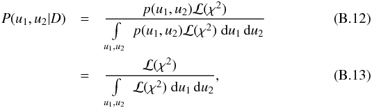 where
p(u1,u2)
represents the prior probability distribution, and the second equality holds for
uniformly distributed priors. Using the expansion of χ2,
the likelihood can be recast as
where
p(u1,u2)
represents the prior probability distribution, and the second equality holds for
uniformly distributed priors. Using the expansion of χ2,
the likelihood can be recast as  (B.14)where
represents the χ2-minimum, and the expression for
Δχ2 has already been derived in Eq. (B.6). Hence, the posterior probability
distribution becomes
(B.14)where
represents the χ2-minimum, and the expression for
Δχ2 has already been derived in Eq. (B.6). Hence, the posterior probability
distribution becomes  (B.15)Here, ℒ0
is a constant that normalizes the posterior. It is found by integration of Eq. (B.15) over Δu1
and Δu2 from −∞ to + ∞, which yields
(B.15)Here, ℒ0
is a constant that normalizes the posterior. It is found by integration of Eq. (B.15) over Δu1
and Δu2 from −∞ to + ∞, which yields
 .
We note that the limits of integration are actually unphysical, because
u1 and u2 are confined to
within an interval reaching from 0 to 1. Additionally,
u1 + u2 must not exceed 1,
which would produce negative brightness on the stellar limb. Nonetheless, we argue
that the approximation is appropriate as long as the Δχ2
ellipse is sufficiently confined.
.
We note that the limits of integration are actually unphysical, because
u1 and u2 are confined to
within an interval reaching from 0 to 1. Additionally,
u1 + u2 must not exceed 1,
which would produce negative brightness on the stellar limb. Nonetheless, we argue
that the approximation is appropriate as long as the Δχ2
ellipse is sufficiently confined.
Parameter correlation is an important aspect in model fitting and error analysis. The
correlation coefficient for u1 and
u2 is given by
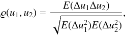 (B.16)where
E denotes the expectation value. The numerator is given by
(B.16)where
E denotes the expectation value. The numerator is given by
![Mathematical equation: \appendix \setcounter{section}{2} \begin{eqnarray} E(\Delta u_1 \Delta u_2) &=& \mathcal{L}_0 \iint \Delta u_1 \Delta u_2 \nonumber \\[3mm] & &\times \mathrm{e}^{-\frac{1}{4}(\Delta u_1^2 A_1 \,+\, \Delta u_2^2 A_2 \,+\, 2\Delta u_1 \Delta u_2 \Delta u_1 A_{12}) } \,\mathrm{d}(\Delta u_1)\,\mathrm{d}(\Delta u_2) \nonumber \\[3mm] &=& \mathcal{L}_0 \int \frac{-2A_{12}\sqrt{\piup}}{A_1^{3/2}}\Delta u_2^2 \mathrm{e}^{-\frac{\Delta u_2^2(A_1A_2 - A_{12}^2)}{4A_1}}\,\mathrm{d}(\Delta u_2) \nonumber \\[3mm] \label{eq:Eu1u2} &=& -\frac{2A_{12}}{A_1A_2 - A_{12}^2} \cdot \end{eqnarray}](/articles/aa/full_html/2013/12/aa22079-13/aa22079-13-eq536.png) (B.17)Similarly,
we derive
(B.17)Similarly,
we derive ![Mathematical equation: \appendix \setcounter{section}{2} \begin{eqnarray} \label{eq:Eu1u1}E(\Delta u_1^2) &=& \frac{2A_2}{A_1A_2 - A_{12}^2} \\[3mm] \label{eq:Eu2u2}E(\Delta u_2^2) &=& \frac{2A_1}{A_1A_2 - A_{12}^2} \cdot \end{eqnarray}](/articles/aa/full_html/2013/12/aa22079-13/aa22079-13-eq537.png) Based
on Eqs. (B.18), (B.19), and (B.17), we obtain the correlation coefficient
Based
on Eqs. (B.18), (B.19), and (B.17), we obtain the correlation coefficient 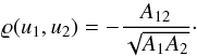 (B.20)We note that the
correlation between u1 and u2
is always negative just by our analytical approach and reaches maximum for
b = 1. The anti-correlated behavior in our simulations is well
reproduced by this analytical solution as can be seen in Fig. B.1.
(B.20)We note that the
correlation between u1 and u2
is always negative just by our analytical approach and reaches maximum for
b = 1. The anti-correlated behavior in our simulations is well
reproduced by this analytical solution as can be seen in Fig. B.1.
The posterior integral over Δu1 or
Δu2, e.g., ![Mathematical equation: \appendix \setcounter{section}{2} \begin{eqnarray} p(\Delta u_1) &=& \mathcal{L}_0 \int \mathrm{e}^{-\frac{1}{4}(\Delta u_1^2 A_1 \,+ \,\Delta u_2^2 A_2\, +\, 2\Delta u_1 \Delta u_2 \Delta u_1 A_{12}) }\,\mathrm{d}(\Delta u_2) \nonumber \\[3mm] \label{eq:Marginal} &=& \mathcal{L}_0 \frac{2 \sqrt{\piup}}{\sqrt{A_2}}\mathrm{e}^{-\frac{\Delta u_1^2(A_1A_2\,-\,A_{12}^2)}{4A_2}} \end{eqnarray}](/articles/aa/full_html/2013/12/aa22079-13/aa22079-13-eq539.png) (B.21)yields
the marginal probability distributions of the parameters. Equation (B.21) shows that the marginal
distributions are Gaussian. Therefore, the width, w, of the 68%
credibility interval is given by
(B.21)yields
the marginal probability distributions of the parameters. Equation (B.21) shows that the marginal
distributions are Gaussian. Therefore, the width, w, of the 68%
credibility interval is given by 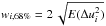 ;
the 95% credibility interval’s width is
wi,95% = 2wi,68%.
Finally, we derive the width of the credibility interval for
Δu1 + Δu2. In particular, we
calculate the variance of
Δu1 + Δu2
;
the 95% credibility interval’s width is
wi,95% = 2wi,68%.
Finally, we derive the width of the credibility interval for
Δu1 + Δu2. In particular, we
calculate the variance of
Δu1 + Δu2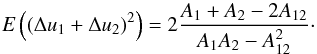 (B.22)The same result is
obtained when applying error propagation considering the correlation of
Δu1 and Δu2. The resulting
error then depends on the correlation coefficient found in Eq. (B.20), which is always negative and close
to −1. This leads to the conclusion that the sum of the anti-correlated parameters
u1 + u2 is always better
constrained than the individual parameters (Fig. 11). For an increasing impact parameter b also the absolute
value of the anti-correlation increases toward its maximum of 1, which leads to
decreasing errors of u1 + u2.
(B.22)The same result is
obtained when applying error propagation considering the correlation of
Δu1 and Δu2. The resulting
error then depends on the correlation coefficient found in Eq. (B.20), which is always negative and close
to −1. This leads to the conclusion that the sum of the anti-correlated parameters
u1 + u2 is always better
constrained than the individual parameters (Fig. 11). For an increasing impact parameter b also the absolute
value of the anti-correlation increases toward its maximum of 1, which leads to
decreasing errors of u1 + u2.
Our result is visualized in Fig. B.1, which shows the development of the measurement errors (left and middle panel) and the correlation (right panel) for different impact parameters b. The points are MCMC results coming from the simulations described in the beginning of this section. The lines show our theoretical predictions using the same planetary parameters and LDCs.
For a more detailed analysis of the correlations of LDCs and other light curve parameters see Pál (2008). Although his model is more complex, his results are consistent with our analysis.
Appendix B.5: Parameter evaluation using correlations
Based on the parameter traces obtained during the MCMC sampling, the covariance
matrix, C, can be estimated, whose elements are the expectation values
![Mathematical equation: \appendix \setcounter{section}{2} \begin{equation} {C}_{i,j} = E\left[(x_i - E(x_i)) (x_j - E(x_j))\right] , \label{eq:covariance} \end{equation}](/articles/aa/full_html/2013/12/aa22079-13/aa22079-13-eq546.png) (B.23)given the
parameters xi and
xj. Using the covariance, we locally
approximate the posterior probability distribution, P, by a
multivariate Gaussian (cf., D’Agostini 2003),
(B.23)given the
parameters xi and
xj. Using the covariance, we locally
approximate the posterior probability distribution, P, by a
multivariate Gaussian (cf., D’Agostini 2003),
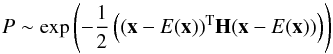 (B.24)and,
therefore,
(B.24)and,
therefore, 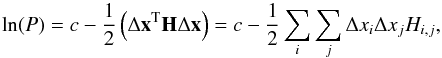 (B.25)where
x is the column vector summarizing the parameter values,
Δx is defined as x − E(x),
H denotes the Hessian matrix, and c is a normalization
constant. The Hessian matrix is the inverse of the covariance matrix,
H = C-1; both matrices are symmetric so that
Hi,j = Hj,i.
(B.25)where
x is the column vector summarizing the parameter values,
Δx is defined as x − E(x),
H denotes the Hessian matrix, and c is a normalization
constant. The Hessian matrix is the inverse of the covariance matrix,
H = C-1; both matrices are symmetric so that
Hi,j = Hj,i.
The derivative with respect to the variable
Δxk reads
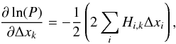 (B.26)and, therefore, the
gradient can be written as
(B.26)and, therefore, the
gradient can be written as 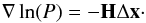 (B.27)We, now, fix one or
more of the offsets, Δxm, to a fixed
value, δm, and adjust the remaining
parameters so that the posterior, P, is again maximized. To that end, we split
Δx into two components, Δy and δ, so that
Δx = Δy + δ. Further, we demand that
δ be a fixed vector of offsets and Δy contains zero
entries for any nonzero element in δ (or offsets fixed to zero). In
this case, the term ΔxTHΔx from Eq.
(B.25) can be rewritten as
(B.27)We, now, fix one or
more of the offsets, Δxm, to a fixed
value, δm, and adjust the remaining
parameters so that the posterior, P, is again maximized. To that end, we split
Δx into two components, Δy and δ, so that
Δx = Δy + δ. Further, we demand that
δ be a fixed vector of offsets and Δy contains zero
entries for any nonzero element in δ (or offsets fixed to zero). In
this case, the term ΔxTHΔx from Eq.
(B.25) can be rewritten as
 (B.28)Defining
b = Hδ, we can write
(B.28)Defining
b = Hδ, we can write 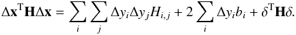 (B.29)By definition, those
Δyi for which
δi is nonzero, i.e., the fixed
parameters, vanish. Therefore, the indices i and j
in Eq. (B.29) only need to cover the
range with nonzero Δym. Using
Δy′,
(B.29)By definition, those
Δyi for which
δi is nonzero, i.e., the fixed
parameters, vanish. Therefore, the indices i and j
in Eq. (B.29) only need to cover the
range with nonzero Δym. Using
Δy′,
Table of deleted transits.
indicating the vector Δy with the zero elements removed,
b′ with the same convention, and H′
with the associated columns and rows removed, we write
 (B.30)The gradient of the
posterior with respect to the variables
Δyi becomes
(B.30)The gradient of the
posterior with respect to the variables
Δyi becomes
 (B.31)The maximum
of the posterior is, thus, found by solving the equation
(B.31)The maximum
of the posterior is, thus, found by solving the equation  (B.32)Evaluating this
expression, we determine how a systematic shift in one or more variables given by
δ affects the remaining parameters,
Δyi.
(B.32)Evaluating this
expression, we determine how a systematic shift in one or more variables given by
δ affects the remaining parameters,
Δyi.
If there are only two variables, of which we fix the first one to
δ1, we find the following expression for the change in
the second, required to maximize the posterior given this constraint:
 (B.33)note that we have not
used primed quantities here. If the variables are entirely uncorrelated
(H2,1 = 0), a change in the first
cannot be compensated by a change in the second. In case of correlations, the
remaining values need to be adapted.
(B.33)note that we have not
used primed quantities here. If the variables are entirely uncorrelated
(H2,1 = 0), a change in the first
cannot be compensated by a change in the second. In case of correlations, the
remaining values need to be adapted.
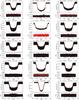 |
Fig. B.2 Top panels: normalized, phase folded transit light curves and best-fit models for the high signal-to-noise sample (Table 1). Bottom panels: residuals for individual data points and overplotted rebinned residuals (red) with one minute bin time. Objects ordered by increasing Teff from the upper left to the lower right corner. |
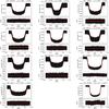 |
Fig. B.2 continued. |
 |
Fig. B.3 Top panels: normalized, phase folded transit light curves and best-fit models for the object sample with high impact parameters (Table 2). Bottom panels: residuals for individual data points and overplotted rebinned residuals (red) with one minute bin time. Objects ordered by Teff from the upper left to the lower right corner. |
For e.g. b = 0.85, the maximum value of μ transited by the planet is μmax ≈ 0.5. Clearly, this does not comply with μ ≪ 1.
Acknowledgments
This paper includes data collected by the Kepler mission. Funding for the Kepler mission is provided by the NASA Science Mission direc- torate. The Kepler observations were obtained from the NASA Mikulski Archive for Space Telescopes (MAST). H.M.M. is supported in the framework of the DFG-funded Research Training Group Extrasolar Planets and their Host Stars (DFG 1351/2).
References
- Alonso, R., Auvergne, M., Baglin, A., et al. 2008, A&A, 482, L21 [NASA ADS] [CrossRef] [EDP Sciences] [Google Scholar]
- Asplund, M., Grevesse, N., Sauval, A. J., & Scott, P. 2009, ARA&A, 47, 481 [NASA ADS] [CrossRef] [Google Scholar]
- Bakos, G. Á., Torres, G., Pál, A., et al. 2010, ApJ, 710, 1724 [NASA ADS] [CrossRef] [Google Scholar]
- Barnes, J. W., Linscott, E., & Shporer, A. 2011, ApJS, 197, 10 [NASA ADS] [CrossRef] [Google Scholar]
- Batalha, N. M., Rowe, J. F., Bryson, S. T., et al. 2013, ApJS, 204, 24 [NASA ADS] [CrossRef] [Google Scholar]
- Bordé, P., Bouchy, F., Deleuil, M., et al. 2010, A&A, 520, A66 [NASA ADS] [CrossRef] [EDP Sciences] [Google Scholar]
- Borucki, W. J., Koch, D. G., Basri, G., et al. 2011, ApJ, 736, 19 [NASA ADS] [CrossRef] [Google Scholar]
- Brown, T. M., Latham, D. W., Everett, M. E., & Esquerdo, G. A. 2011, AJ, 142, 112 [NASA ADS] [CrossRef] [Google Scholar]
- Buchhave, L. A., Latham, D. W., Johansen, A., et al. 2012, Nature, 486, 375 [NASA ADS] [Google Scholar]
- Caffau, E., Steffen, M., Sbordone, L., Ludwig, H.-G., & Bonifacio, P. 2007, A&A, 473, L9 [NASA ADS] [CrossRef] [EDP Sciences] [Google Scholar]
- Carter, J. A., & Winn, J. N. 2009, ApJ, 704, 51 [NASA ADS] [CrossRef] [Google Scholar]
- Carter, J. A., Yee, J. C., Eastman, J., Gaudi, B. S., & Winn, J. N. 2008, ApJ, 689, 499 [NASA ADS] [CrossRef] [Google Scholar]
- Casagrande, L., Schönrich, R., Asplund, M., et al. 2011, A&A, 530, A138 [NASA ADS] [CrossRef] [EDP Sciences] [Google Scholar]
- Charbonneau, D., Brown, T. M., Latham, D. W., & Mayor, M. 2000, ApJ, 529, L45 [NASA ADS] [CrossRef] [PubMed] [Google Scholar]
- Claret, A. 2000, A&A, 363, 1081 [NASA ADS] [Google Scholar]
- Claret, A. 2008, A&A, 482, 259 [NASA ADS] [CrossRef] [EDP Sciences] [Google Scholar]
- Claret, A., & Bloemen, S. 2011, A&A, 529, A75 [NASA ADS] [CrossRef] [EDP Sciences] [Google Scholar]
- Csizmadia, S., Pasternacki, T., Dreyer, C., et al. 2013, A&A, 549, A9 [NASA ADS] [CrossRef] [EDP Sciences] [Google Scholar]
- Daemgen, S., Hormuth, F., Brandner, W., et al. 2009, A&A, 498, 567 [NASA ADS] [CrossRef] [EDP Sciences] [Google Scholar]
- D’Agostini, G. 2003, Rep. Prog. Phys., 66, 1383 [Google Scholar]
- Demarque, P., Woo, J.-H., Kim, Y.-C., & Yi, S. K. 2004, ApJS, 155, 667 [NASA ADS] [CrossRef] [Google Scholar]
- Désert, J.-M., Charbonneau, D., Demory, B.-O., et al. 2011, ApJS, 197, 14 [NASA ADS] [CrossRef] [Google Scholar]
- Fressin, F., Torres, G., Charbonneau, D., et al. 2013, ApJ, 766, 81 [NASA ADS] [CrossRef] [Google Scholar]
- Hampel, F. R. 1974, J. Am. Stat. Assoc., 69, 383 [CrossRef] [Google Scholar]
- Haubois, X., Perrin, G., Lacour, S., et al. 2009, A&A, 508, 923 [NASA ADS] [CrossRef] [EDP Sciences] [Google Scholar]
- Hauschildt, P. H., & Baron, E. 2010, A&A, 509, A36 [NASA ADS] [CrossRef] [EDP Sciences] [Google Scholar]
- Hayek, W., Sing, D., Pont, F., & Asplund, M. 2012, A&A, 539, A102 [NASA ADS] [CrossRef] [EDP Sciences] [Google Scholar]
- Heyrovský, D. 2007, ApJ, 656, 483 [NASA ADS] [CrossRef] [Google Scholar]
- Howarth, I. D. 2011a, MNRAS, 413, 1515 [NASA ADS] [CrossRef] [Google Scholar]
- Howarth, I. D. 2011b, MNRAS, 418, 1165 [NASA ADS] [CrossRef] [Google Scholar]
- Huber, K. F., Czesla, S., Wolter, U., & Schmitt, J. H. M. M. 2010, A&A, 514, A39 [NASA ADS] [CrossRef] [EDP Sciences] [Google Scholar]
- Jones, E., Oliphant, T., Peterson, P., et al. 2001, SciPy: Open source scientific tools for Python, http://www.scipy.org [Google Scholar]
- Kipping, D., & Bakos, G. 2011a, ApJ, 730, 50 [NASA ADS] [CrossRef] [Google Scholar]
- Kipping, D., & Bakos, G. 2011b, ApJ, 733, 36 [NASA ADS] [CrossRef] [Google Scholar]
- Knutson, H. A., Charbonneau, D., Noyes, R. W., Brown, T. M., & Gilliland, R. L. 2007, ApJ, 655, 564 [NASA ADS] [CrossRef] [Google Scholar]
- Kopal, Z. 1950, Harvard College Observatory Circular, 454, 1 [Google Scholar]
- Mandel, K., & Agol, E. 2002, ApJ, 580, L171 [NASA ADS] [CrossRef] [Google Scholar]
- Neckel, H., & Labs, D. 1994, Sol. Phys., 153, 91 [NASA ADS] [CrossRef] [Google Scholar]
- Nesvacil, N., Lüftinger, T., Shulyak, D., et al. 2012, A&A, 537, A151 [NASA ADS] [CrossRef] [EDP Sciences] [Google Scholar]
- Ohta, Y., Taruya, A., & Suto, Y. 2005, ApJ, 622, 1118 [NASA ADS] [CrossRef] [Google Scholar]
- Pál, A. 2008, MNRAS, 390, 281 [NASA ADS] [CrossRef] [Google Scholar]
- Pál, A., Bakos, G. Á., Torres, G., et al. 2008, ApJ, 680, 1450 [NASA ADS] [CrossRef] [Google Scholar]
- Patil, A., Huard, D., & Fonnesbeck, C. J. 2010, J. Stat. Software, 35, 1 [Google Scholar]
- Pont, F., Zucker, S., & Queloz, D. 2006, MNRAS, 373, 231 [NASA ADS] [CrossRef] [Google Scholar]
- Press, W. H., Teukolsky, S. A., Vetterling, W. T., & Flannery, B. P. 2002, Numerical recipes in C++: the art of scientific computing (Cambridge University Press) [Google Scholar]
- Russell, I. H. N., & Shapley, H. 1912, ApJ, 36, 239 [NASA ADS] [CrossRef] [Google Scholar]
- Sanchis-Ojeda, R., & Winn, J. N. 2011, ApJ, 743, 61 [NASA ADS] [CrossRef] [Google Scholar]
- Schröter, S., Schmitt, J. H. M. M., & Müller, H. M. 2012, A&A, 539, A97 [NASA ADS] [CrossRef] [EDP Sciences] [Google Scholar]
- Schwarzschild, K. 1906, Nachrichten von der Gesellschaft der Wissenschaften zu Göttingen, Mathematisch-Physikalische Klasse, 41 [Google Scholar]
- Sing, D. K. 2010, A&A, 510, A21 [Google Scholar]
- Soubiran, C., Le Campion, J.-F., Cayrel de Strobel, G., & Caillo, A. 2010, A&A, 515, A111 [NASA ADS] [CrossRef] [EDP Sciences] [Google Scholar]
- Southworth, J. 2008, MNRAS, 386, 1644 [NASA ADS] [CrossRef] [Google Scholar]
- Szabó, G. M., Szabó, R., Benkő, J. M., et al. 2011, ApJ, 736, L4 [NASA ADS] [CrossRef] [Google Scholar]
- Trampedach, R., Asplund, M., Collet, R., Nordlund, Å., & Stein, R. F. 2013, ApJ, 769, 18 [NASA ADS] [CrossRef] [Google Scholar]
- Valenti, J. A., & Piskunov, N. 1996, A&AS, 118, 595 [NASA ADS] [CrossRef] [EDP Sciences] [Google Scholar]
- van Hamme, W. 1993, AJ, 106, 2096 [NASA ADS] [CrossRef] [Google Scholar]
- Wade, R. A., & Rucinski, S. M. 1985, A&AS, 60, 471 [NASA ADS] [Google Scholar]
- Wedemeyer, S., Freytag, B., Steffen, M., Ludwig, H.-G., & Holweger, H. 2004, A&A, 414, 1121 [NASA ADS] [CrossRef] [EDP Sciences] [Google Scholar]
All Tables
All Figures
|
Fig. 1 Kepler signal-to-noise ratios (SNR) of short cadence planetary candidates as of 2012/02/27, versus number of transit data points per day (Np). Large markers indicate our target selection. Diamonds: high signal-to-noise sample (SNR ≥ 1000), big circles: sample with high impact parameters b ≥ 0.8 (SNR ≥ 150). |
| In the text | |
|
Fig. 2 Normalized and phase-folded transit light curve of HAT-P-11b. The manually deleted transit light curves are included, clearly visible above our best-fit model shown in red. This model only uses 18 out of 95 transits (see Table B.1). |
| In the text | |
|
Fig. 3 Normalized and phase-folded transit light curve of HAT-P-7b. Ten manually deleted transit light curves are included. |
| In the text | |
|
Fig. 4 Normalized and phase-folded transit light curve of KIC 9631995. Eight manually deleted transit light curves are included in this figure. |
| In the text | |
|
Fig. 5 Quadratic LDCs determined by MCMC for our high signal-to-noise target sample (see Table 1). For comparison, the graphs show model predictions based on PHOENIX (solid) and ATLAS (dashed) atmospheric models, taken from Claret & Bloemen (2011). The dotted lines show Claret and Bloemen’s LDCs determined for the same atmospheres by different methods (see Sect. 5.1). The diamond symbol indicates TrES-2, which has the highest impact parameter of this sample (b = 0.845). Triangles mark conspicuous objects, discussed in Sect. 5.3. |
| In the text | |
|
Fig. 6 Sum of the linear and quadratic limb-darkening coefficients for objects with an impact parameter b < 0.8 of our high signal-to-noise sample in comparison to the summed model predictions (solid: PHOENIX, dashed: ATLAS). |
| In the text | |
|
Fig. 7 Same as Fig. 5 for objects with impact parameters larger than 0.8 as given in the Kepler planetary candidates list (i.e. our high-impact-parameter sample, see Table 2). According to our transit modeling only objects marked with diamonds truly have b ≥ 0.8 while we found b < 0.8 for the objects indicated by dots. |
| In the text | |
|
Fig. 8 Summed quadratic deviation of measured LD coefficients from those calculated from PHOENIX models versus impact parameter. |
| In the text | |
|
Fig. 9 Summed width of the 68.3% HPD intervals for u1 and u2 versus the impact parameter b as determined by MCMC. See text for details. |
| In the text | |
|
Fig. 10 Sum of the linear and quadratic coefficients uC = u1 + u2 for objects with an impact parameter b > 0.8 in comparison to the summed model predictions (solid: PHOENIX, dashed: ATLAS). |
| In the text | |
|
Fig. 11 Simulated measurement errors (dots) for the individual LDCs u1 (cyan), u2 (purple) and for the sum u1 + u2 (green) as determined by transit modeling. For the simulation we used fixed parameters only the impact parameter was varied between 0 and 1. The overplotted lines show our analytical solutions (see Appendix B for details). |
| In the text | |
|
Fig. A.1 Influence of log (g) on the LDC u1. Shown is the difference between u1 determined with log (g) = 4.5 and values of u1 using a higher (4.8) and lower (4.3) surface gravity, over a wide temperature range (ATLAS models). |
| In the text | |
|
Fig. A.2 Influence of the stellar metallicity on u1. Differences between u1 determined with [M/H] = 0.0 and values of u1 using different metallicities are plotted against Teff (ATLAS models). |
| In the text | |
|
Fig. B.1 Comparison of simulations (dots) and our analytical solutions (lines). Left and center: dependency of the measurement errors on the system impact parameter b. Right: correlation coefficients of the LDCs with increasing b. See Sect. B.4 for details. |
| In the text | |
|
Fig. B.2 Top panels: normalized, phase folded transit light curves and best-fit models for the high signal-to-noise sample (Table 1). Bottom panels: residuals for individual data points and overplotted rebinned residuals (red) with one minute bin time. Objects ordered by increasing Teff from the upper left to the lower right corner. |
| In the text | |
|
Fig. B.2 continued. |
| In the text | |
|
Fig. B.3 Top panels: normalized, phase folded transit light curves and best-fit models for the object sample with high impact parameters (Table 2). Bottom panels: residuals for individual data points and overplotted rebinned residuals (red) with one minute bin time. Objects ordered by Teff from the upper left to the lower right corner. |
| In the text | |
Current usage metrics show cumulative count of Article Views (full-text article views including HTML views, PDF and ePub downloads, according to the available data) and Abstracts Views on Vision4Press platform.
Data correspond to usage on the plateform after 2015. The current usage metrics is available 48-96 hours after online publication and is updated daily on week days.
Initial download of the metrics may take a while.