| Issue |
A&A
Volume 560, December 2013
|
|
|---|---|---|
| Article Number | A53 | |
| Number of page(s) | 5 | |
| Section | Cosmology (including clusters of galaxies) | |
| DOI | https://doi.org/10.1051/0004-6361/201220971 | |
| Published online | 05 December 2013 | |
Research Note
Mass-varying neutrino in light of cosmic microwave background and weak lensing
1 Physics Department “G. Occhialini”Milano-Bicocca University and I.N.F.N., 20126 Milano, Italy
e-mail: This email address is being protected from spambots. You need JavaScript enabled to view it.
2 Institute of Theoretical Astrophysics, University of Oslo, 0315 Oslo, Norway
Received: 20 December 2012
Accepted: 23 September 2013
Abstract
Aims. We aim to constrain mass-varying neutrino models using large scale structure observations and produce forecast for the Euclid survey.
Methods. We investigate two models with different scalar field potential and both positive and negative coupling parameters β. These parameters correspond to growing or decreasing neutrino mass, respectively. We explore couplings up to | β | ≲ 5.
Results. In the case of the exponential potential, we find an upper limit on Ωνh2 < 0.004 at 2σ level. In the case of the inverse power law potential the null coupling can be excluded with more than 2σ significance; the limits on the coupling are β > 3 for the growing neutrino mass and β < − 1.5 for the decreasing mass case. This is a clear sign for a preference of higher couplings. When including a prior on the present neutrino mass the upper limit on the coupling becomes | β | < 3 at 2σ level for the exponential potential. Finally, we present a Fisher forecast using the tomographic weak lensing from an Euclid-like experiment and we also consider the combination with the cosmic microwave background (CMB) temperature and polarisation spectra from a Planck-like mission. If considered alone, lensing data is more efficient in constraining Ων with respect to CMB data alone. There is, however, a strong degeneracy in the β-Ωνh2 plane. When the two data sets are combined, the latter degeneracy remains, but the errors are reduced by a factor ~2 for both parameters.
Key words: cosmology: theory / dark energy / neutrinos
© ESO, 2013
1. Introduction
We study models in which the dark energy (DE) field is coupled to neutrinos (Bjaelde et al. 2008; Brookfield et al. 2006b,a; Amendola et al. 2008; Pettorino et al. 2009). Several authors have shown that important cosmological effects can appear within this class of models, especially when the neutrino mass is sufficiently big for neutrinos to be non-relativistic (Wintergerst et al. 2010; Mota et al. 2008; Pettorino et al. 2010). In this work, we further investigate the cosmological signatures of the mass-varying neutrino (MaVaN) models and put constraints on them using the most updated observational data from the cosmic microwave background (CMB) radiation temperature anisotropies spectra, from the large scale structure (LSS), and the supernovae type Ia (SNIa) luminosity distance. We start by investigating two different scalar field potentials and both positive and negative coupling parameters. These parameters corresponds to growing or decreasing neutrino mass, respectively. Finally, we present a Fisher forecast using the tomographic weak lensing from an Euclid-like experiment (Laureijs et al. 2011) in the last section. This is also shown in combination with the CMB temperature and polarisation spectra from a Planck-like mission (Planck Collaboration 2006).
2. The cosmological background evolution
The MaVaN models involve a coupling between the DE scalar field and massive neutrinos. The coupling of DE to the neutrinos results in the neutrino mass becoming a function of the scalar field,  (1)where
  is a constant. An additional attractive force between neutrinos of strength 2β2 is mediated by the scalar field exchange. The DE and mass varying neutrinos obey the coupled conservation equations:
  where the energy density and pressure stored in the neutrinos is given by
  (4)Here f0(q) is the usual unperturbed background neutrino Fermi-Dirac distribution function:
  (5)and
  (q denotes the comoving momentum). As usual, gs, hP, and kB stand for the number of spin degrees of freedom, Planck constant, and Boltzmann constant, respectively.
Taking the energy conservation of the coupled neutrino-dark energy system into account, one can immediately find that the evolution of the scalar field is described by a modified Klein-Gordon equation:  (6)Here we investigate two different expressions for the DE potentials, an exponential potential (Wetterich 1988) and an inverse power-law (Binetruy 1999):
  (7)The initial conditions for the field φ and its time derivative are chosen in a recursive way to reproduce the correct value of the assigned density parameters at a = 1. In the very early universe, neutrinos are still relativistic and almost massless, where pν = ρν/3 and the coupling term in Eqs. (2), (3), (6) vanishes. However, the coupling term ~βρν becomes significantly different from zero as soon as neutrinos become nonrelativistic, affecting the evolution of the field φ. Neutrinos and φ densities change behaviour for z < 6: the value of the scalar field stays almost constant, and the frozen scalar field potential mimics a cosmological constant. According to this model, neutrinos at the present time are still subdominant with respect to cold dark matter (CDM), though they will take the lead in the future. For our choice of the parameters, neutrino pressure terms may be safely neglected for redshifts znr < 4; before that, redshift neutrinos free stream as usual relativistic particles.
2.1. Perturbed equations
The perturbed Klein-Gordon equation is given by (Brookfield et al. 2006b): ![Mathematical equation: \begin{eqnarray} \label{pertkg} \lefteqn{\ddot{\delta \phi}+ 2H \dot{\delta \phi}+\left(k^{2} + a^{2}\frac{{\rm d}^{2}V}{{\rm d} \phi^{2}}\right)\delta \phi+\frac{1}{2}\dot{h} \dot{\phi}=} \\ \nonumber & &-a^2 \left[\frac{{\rm d}\ln m_\nu}{{\rm d}\phi}(\delta\rho_\nu-3\delta p_\nu)+\frac{{\rm d}^{2} \ln m_\nu}{{\rm d}\phi^{2}}\delta\phi(\rho_\nu-3 p_\nu)\right]. \end{eqnarray}](/articles/aa/full_html/2013/12/aa20971-12/aa20971-12-eq31.png) (8)For the neutrinos, we use the perturbed component of the energy momentum conservation equation for the coupled neutrinos
(8)For the neutrinos, we use the perturbed component of the energy momentum conservation equation for the coupled neutrinos  , whilst taking γ = i (spatial index) yields the velocity perturbation equation
  with the coordinate velocity
  /dτ:
/dτ: 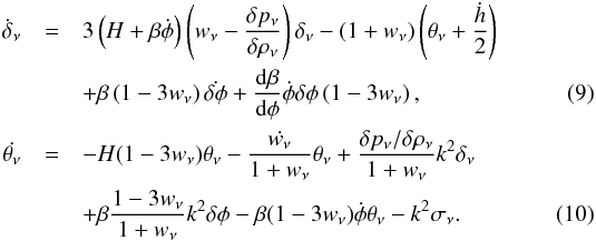
3. Methods and data
In this paper, we use two methods to test MaVaN theory against cosmological data: the likelihood analysis through Markov-chain Monte-Carlo (MCMC) technique and the Fisher information matrix.
The CMB anisotropy and matter power spectra are calculated by suitably modifying CAMB (Lewis et al. 2000) to include MaVaN’s equations as described above. To ensure the accuracy of our calculations, we directly integrate the neutrino distribution function, rather than using the standard velocity weighted series approximation scheme.
For the MCMC analysis, we use a modified version of the publicly available codes CosmoMC (Lewis & Bridle 2002) to explore the parameter space. We consider the following basic set of parameters:
 and also σ when the exponential potential is involved. Here, ωb, ωCDM, ων are the physical baryon, cold dark matter, and neutrino density parameters. Here, ωi = Ωih2, where i = b, CDM, ν, and h is the dimensionless Hubble parameter H0; zre is the redshift of reionization; ns is the scalar spectral index; As denotes the amplitude of the scalar fluctuations at a scale of k = 0.05 Mpc-1. The sum of the ν masses is directly related to the neutrino density parameter through the relation Mν = Σmν = ων·93.5 eV, assuming three equal mass ν values.
All parameters are given flat priors, unless otherwise stated explicitly. We separately consider positive and negative β values in Eq. (1), which correspond to either a growing or decreasing neutrino mass, respectively. We choose to span only the low coupling regime up to | β | < 5, since linear perturbations become unstable for high couplings, e.g. | β | ~ 50 (Mota et al. 2008; Wintergerst et al. 2010). In our MCMC analysis, we assume that the Universe is spatially flat.
With the aim of obtaining the best estimate of the cosmological parameters, we combine different CMB data sets (WMAP (Komatsu et al. 2011), CBI (Sievers et al. 2007), ACBAR (Reichardt et al. 2009), VSA (Dickinson et al. 2004)) with data from LSS (Tegmark et al. 2006) and SNIa (Amanullah et al. 2010). We also apply additional priors on the Hubble parameter of H0 = 74.2 ± 3.6 (Riess et al. 2009).
In addition to the likelihood analysis, we test the power of future CMB and weak-lensing data by constraining MaVaN’s parameters using the Fisher formalism (Fisher 1935; Tegmark et al. 1997).
4. MCMC results
In the case of the exponential potential (7), the plots for ων, σ, and β are shown in Fig. 1. For both a growing and decreasing mass, no stringent constraints can be put on the coupling β, whose upper limit exceeds | β | = 5 at 68% confidence level (CL). In contrast, the ν density parameter is well constrained at 95% CL: ων < 0.0034 (ων < 0.0032) for a decreasing (growing) mass. These limits are ~3 times narrower than those found in Brookfield et al. (2006b). In terms of current neutrino mass these values result in an upper limit to mν ≃ 0.32 eV. We note here that the results show a common behaviour in the β vs. ων plots, which are almost symmetric with respect to the sign of β. A degeneracy appears between the two parameters, so that a high | β | agrees with low neutrino content, or, equivalently, low neutrino mass.
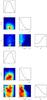 |
Fig. 1 In the upper (lower) panel, likelihood contours and distributions are shown for decreasing (growing) neutrino mass in the exponential potential case. For the plots on the diagonal, dotted (solid) lines are mean (marginalized) likelihoods of samples. Similarly, black lines on the plots exhibit 1- and 2σ contours of the marginalised probability distribution, while the colours refer to the mean likelihood degradation from the top (dark red) to lower values. |
In Fig. 2, we reported likelihood contours for the case of the inverse power-law potential. This potential type was not previously considered in Brookfield et al. (2006b). In the β vs. ων, plots the zero coupling is apparently excluded with statistical significance that is higher than 95% confidence level (CL), with β > 3 for the growing neutrino mass and β < − 1.5 for the decreasing mass case at 2σ. In particular, the growing neutrino mass case exhibits an explicit preference for high β values, which agree with Amendola et al. (2008). For ων, only upper limits can be found at 95% CL: ων < 0.0017 (ων < 0.0423) for decreasing (growing) mass.
To exploit complementary information from external measurements, we performed a specific analysis, by fixing the current neutrino mass value using two possible options, mν = 0.2 eV and mν = 0.3 eV. These values are within the range of the claimed νe mass detection in the Heidelberg-Moscow experiment (Klapdor-Kleingrothaus et al. 2004; Klapdor-Kleingrothaus 2005). The KATRIN experiment (Sturm 2011) is also expected to constrain the value of the neutrino mass with a sensitivity in the sub-eV range. Besides fixing ων, we chose to fix Ωbh2 = 0.022, as constraints on this parameter are not significantly modified by neutrino-DE couplings, and H0 = 72 km s-1 Mpc-1.
As shown in Figs. 3 and 4, the most significant result is the improvement in the limits on the coupling | β |, which has an upper value of the order between 2 or 3, and the distributions for σ become narrower, but are always compatible with zero at 68% CL. The complex structure for the likelihood contours in the upper panel of Fig. 3 can be mainly ascribed to the peculiar features of the likelihood in Fig. 1, which are completely lost when considering a prior with higher mass.
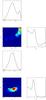 |
Fig. 3 Upper (lower) panel shows posterior constraints for the exponential potential with growing ν mass. Here we fixed mν = 0.2 eV (mν = 0.3 eV), ωb = 0.022, H0 = 72. |
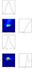 |
Fig. 4 Upper (lower) panel shows posterior constraints for the exponential potential with decreasing ν mass. Here we fixed mν = 0.2 eV (mν = 0.3 eV), ωb = 0.022, H0 = 72. |
5. Fisher matrix forecasts
In this section, we show Fisher matrix results from the combination of the CMB anisotropies and the tomographic weak lensing (TWL) spectra. We considered the exponential potential with an exponential coupling. The fiducial parameters θα are shown in Table 1. These two sets correspond to the maximum area of the likelihood as determined above and are chosen to be exactly the same, except for the sign of β.
The Fisher matrix for CMB power spectrum (Zaldarriaga & Seljak 1997; Zaldarriaga et al. 1997; Rassat et al. 2008) is calculated using Planck mission (Planck Collaboration 2006) specifications. We assume that we only use the 143 GHz channel as the science channel. This channel has a beam of θfwhm = 7.1′ and sensitivities of σT = 2.2μK/K and σP = 4.2μK/K. To account for the galactic plane cut, we take fsky = 0.80. Note that we use ℓmin = 30 as a minimum ℓ-mode to avoid problems with polarization foregrounds and subtleties when modelling of the integrated Sachs-Wolfe effect.
The Fisher matrix for TWL (Hu & Jain 2004) is calculated using the forthcoming Euclid mission1 specifications (Laureijs et al. 2011). The survey area covered by the experiment is 15 000 deg2, while the density is 30 galaxies per arcmin2. The distribution of the galaxy number on the redshift and solid angle is n(z) = n0z2e− (z/z0)1.5 with a median redshift  . The photometric redshift error is 0.05 (1 + z). We consider the five bin case as reference case. Non-linear corrections of the matter power spectra are calculated using halofit (Smith et al. 2003). Since this procedure is suitably fitted to ΛCDM N-body simulations, it can lead to errors of the order of 20% on Fisher outputs, if used for models different from ΛCDM (see e.g. Casarini et al. 2011). However, we use halofit in the absence of suitable extensions for MaVaN, and report results up to ℓmax = 1000 in the mildly non-linear regime. This conservative choice also prevents us from the effects of baryons on the matter power spectra and weak-lensing spectra (Casarini et al. 2012).
1-σ error estimations of cosmological parameters for an exponential potential with β < 0, using Planck-like CMB and Euclid-like tomographic weak lensing (TWL) data.
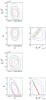 |
Fig. 5 Upper (lower) panel shows 68% and 95% likelihood confidence levels for the exponential potential, in the decreasing (growing) mass case. The green lines are obtained considering an Euclid-like TWL survey. The blue lines are for a Planck-like CMB mission. The red lines are for the combination of the two. |
As shown in Table 2, TWL is able to put constraints stronger than CMB on β < 0 and ων, with an improvement of ~10% and >30%, respectively. Instead CMB is more efficient in constraining σ, gaining ~50% over TWL. The combination of the two observables can improve constraints on all parameters. Analogous comments can be made for the β > 0 in Table 3 with the only difference that CMB can constrain β better than TWL.
In Fig. 5, we show 1σ and 2σ likelihood contours for ων, β and σ, after marginalising over the other parameters. It is clear that neither Planck nor Euclid alone can be able to constrain a non-zero coupling  ; only TWL is slightly more efficient than CMB in the β < 0 case. In this case the combination of the two can exclude a null coupling with a significance higher than 2σ. We note that higher multipoles can significantly reduce the limits on β and the other parameters. If we suppose, for instance, that halofit is appropriate for our models at multipoles up to ℓmax = 5000 in the TWL Fisher matrix (see Fig. 6), the estimated errors are then clearly reduced with a factor ~2 with respect to Fig. 6. In this case, Euclid would be able to exclude the zero value both for β and ων with high statistical significance.
Despite this limitation, a very interesting result is that TWL, whether alone or in combination with CMB, is able to find a lower value of Ωνh2 with an error that is half of the CMB error if taken alone. Moreover, a strong degeneracy can be found in the ων-β plane with regard to the TWL ellipses and also in combination with CMB. This effect appears in both cases in a symmetric way, showing that lower | β | values allow higher neutrino mass. The Ωνh2-β degeneracy could be eventually broken from external priors on mν. On the other hand, no noteworthy remark can be said about the σ parameter, whose constrain remains compatible with zero for the combination of the two observables.
6. Discussion and conclusions
In this work, we focused on the hypothesis that the origin of cosmic acceleration can be attributed to a quintessence scalar field coupled to massive neutrinos. First, we updated and extended parameter constraints using the most recent available data from SNIa, CMB, and LSS observations. We considered both an exponential and a power law potential with growing (β > 0) or decreasing (β < 0) neutrino mass.
The cosmological data did not place strong constraints on the coupling parameter in the low coupling range or for the neutrino density parameter, on which only upper limits can be placed in any of these cases. The main outcome of the analysis was that β values ~ are compatible with actual data with a neutrino mass mν ≲ 0.32 eV.
Therefore we do have not enough information at the moment to exclude a possible coupling between the neutrino and DE field in either the low or the high coupling regime. New and precise data from observables related to the recent evolution of the universe are necessary with a deeper understanding of the MaVaN theory dynamics. In this sense, the forthcoming Euclid weak-lensing and galaxy clustering data represent the turning point for the future progress in cosmology.
With this aim, a Fisher matrix study was accomplished by considering future data release from missions, such as Planck for CMB spectra and Euclid for tomographic weak lensing spectra. The latter experiment is more efficient in improving present constraints on ων, even considering a cautious use of multipoles up to ℓmax = 1000. This choice prevents us from including highly non-linear features, which are not correctly predicted by halofit for MaVaN theories. Combining Euclid data with complementary information from Planck reduces the estimated error to about a factor 2 with respect to considering the two datasets alone. It is worth to mention that the strong degeneracy between β and ων could eventually be broken by an external prior on the neutrino mass.
A crucial point for the forthcoming Euclid mission is to study and implement an efficient way of including non-linear corrections on the matter power spectrum calculations with halofit being only suitable for ΛCDM cosmologies. Delving into the deep non-linear regime of matter perturbations could significantly improve parameter estimation by fully exploiting the high potentiality of the TWL from Euclid.
Acknowledgments
D.F.M. thanks the Research Council of Norway.
References
- Amanullah, R., Lidman, C., Rubin, D., et al. 2010, ApJ, 716, 712 [NASA ADS] [CrossRef] [Google Scholar]
- Amendola, L., Baldi, M., & Wetterich, C. 2008, Phys. Rev. D, 78, 023015 [NASA ADS] [CrossRef] [Google Scholar]
- Binetruy, P. 1999, Phys. Rev. D, 60, 063502 [NASA ADS] [CrossRef] [Google Scholar]
- Bjaelde, O. E., Brookfield, A. W., van de Bruck, C., et al. 2008, JCAP, 0801, 026 [CrossRef] [Google Scholar]
- Brookfield, A., van de Bruck, C., Mota, D., & Tocchini-Valentini, D. 2006a, Phys. Rev. Lett., 96, 061301 [NASA ADS] [CrossRef] [MathSciNet] [PubMed] [Google Scholar]
- Brookfield, A. W., van de Bruck, C., Mota, D., & Tocchini-Valentini, D. 2006b, Phys. Rev. D, 73, 083515 [NASA ADS] [CrossRef] [Google Scholar]
- Casarini, L., La Vacca, G., Amendola, L., Bonometto, S. A., & Maccio, A. V. 2011, JCAP, 1103, 026 [NASA ADS] [CrossRef] [Google Scholar]
- Casarini, L., Bonometto, S. A., Borgani, S., et al. 2012, A&A, 542, A126 [NASA ADS] [CrossRef] [EDP Sciences] [Google Scholar]
- Dickinson, C., Battye, R. A., Carreira, P., et al. 2004, MNRAS, 353, 732 [NASA ADS] [CrossRef] [Google Scholar]
- Fisher, R. A. 1935, J. Roy. Statist. Soc., 98, 39 [Google Scholar]
- Hu, W., & Jain, B. 2004, Phys. Rev. D, 70, 043009 [NASA ADS] [CrossRef] [Google Scholar]
- Klapdor-Kleingrothaus, H. V. 2005, in Proc. of XI Int. Work. on Neutrino Telescopes, Febr. 22–25, Venice, Italy, ed. M. Baldo-Ceolin, Padova Univ., 215 [Google Scholar]
- Klapdor-Kleingrothaus, H., Krivosheina, I., Dietz, A., & Chkvorets, O. 2004, Phys. Lett. B, 586, 198 [NASA ADS] [CrossRef] [Google Scholar]
- Komatsu, E., Smith, K. M., Dunkley, J., et al. 2011, ApJS, 192, 18 [NASA ADS] [CrossRef] [Google Scholar]
- Laureijs, R., Amiaux, J., Arduini, S., et al. 2011 [arXiv:1110.3193] [Google Scholar]
- Lewis, A., & Bridle, S. 2002, Phys. Rev. D, 66, 103511 [NASA ADS] [CrossRef] [Google Scholar]
- Lewis, A., Challinor, A., & Lasenby, A. 2000, ApJ, 538, 473 [NASA ADS] [CrossRef] [Google Scholar]
- Mota, D., Pettorino, V., Robbers, G., & Wetterich, C. 2008, Phys. Lett. B, 663, 160 [NASA ADS] [CrossRef] [Google Scholar]
- Pettorino, V., Mota, D. F., Robbers, G., & Wetterich, C. 2009, AIP Conf. Proc., 1115, 291 [NASA ADS] [CrossRef] [Google Scholar]
- Pettorino, V., Wintergerst, N., Amendola, L., & Wetterich, C. 2010, Phys. Rev. D, 82, 123001 [NASA ADS] [CrossRef] [Google Scholar]
- Planck Collaboration 2006 [arXiv:astro-ph/0604069] [Google Scholar]
- Rassat, A., Amara, A., Amendola, L., et al. 2008, MNRAS, submitted [arXiv:0810.0003] [Google Scholar]
- Reichardt, C., Ade, P., Bock, J., et al. 2009, ApJ, 694, 1200 [NASA ADS] [CrossRef] [Google Scholar]
- Riess, A. G., Macri, L., Casertano, S., et al. 2009, ApJ, 699, 539 [NASA ADS] [CrossRef] [Google Scholar]
- Sievers, J. L., Achermann, C., Bond, J., et al. 2007, ApJ, 660, 976 [NASA ADS] [CrossRef] [Google Scholar]
- Smith, R., Peacock, J. A., Jenkins, A., et al. 2003, MNRAS, 341, 1311 [NASA ADS] [CrossRef] [Google Scholar]
- Sturm, M. 2011 [arXiv:1111.4773] [Google Scholar]
- Tegmark, M., Taylor, A., & Heavens, A. 1997, ApJ, 480, 22 [NASA ADS] [CrossRef] [Google Scholar]
- Tegmark, M., Eisenstein, D. J., Strauss, M. A., et al. 2006, Phys. Rev. D, 74, 123507 [Google Scholar]
- Wetterich, C. 1988, Nucl. Phys. B, 302, 645 [NASA ADS] [CrossRef] [Google Scholar]
- Wintergerst, N., Pettorino, V., Mota, D., & Wetterich, C. 2010, Phys. Rev. D, 81, 063525 [NASA ADS] [CrossRef] [Google Scholar]
- Zaldarriaga, M., & Seljak, U. 1997, Phys. Rev. D, 55, 1830 [Google Scholar]
- Zaldarriaga, M., Spergel, D. N., & Seljak, U. 1997, ApJ, 488, 1 [NASA ADS] [CrossRef] [Google Scholar]
All Tables
1-σ error estimations of cosmological parameters for an exponential potential with β < 0, using Planck-like CMB and Euclid-like tomographic weak lensing (TWL) data.
All Figures
|
Fig. 1 In the upper (lower) panel, likelihood contours and distributions are shown for decreasing (growing) neutrino mass in the exponential potential case. For the plots on the diagonal, dotted (solid) lines are mean (marginalized) likelihoods of samples. Similarly, black lines on the plots exhibit 1- and 2σ contours of the marginalised probability distribution, while the colours refer to the mean likelihood degradation from the top (dark red) to lower values. |
| In the text | |
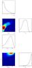 |
Fig. 2 As in Fig. 1, when the power-law potential is considered. |
| In the text | |
|
Fig. 3 Upper (lower) panel shows posterior constraints for the exponential potential with growing ν mass. Here we fixed mν = 0.2 eV (mν = 0.3 eV), ωb = 0.022, H0 = 72. |
| In the text | |
|
Fig. 4 Upper (lower) panel shows posterior constraints for the exponential potential with decreasing ν mass. Here we fixed mν = 0.2 eV (mν = 0.3 eV), ωb = 0.022, H0 = 72. |
| In the text | |
|
Fig. 5 Upper (lower) panel shows 68% and 95% likelihood confidence levels for the exponential potential, in the decreasing (growing) mass case. The green lines are obtained considering an Euclid-like TWL survey. The blue lines are for a Planck-like CMB mission. The red lines are for the combination of the two. |
| In the text | |
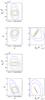 |
Fig. 6 As in Fig. 5 with 5 bins and ℓmax = 5000. |
| In the text | |
Current usage metrics show cumulative count of Article Views (full-text article views including HTML views, PDF and ePub downloads, according to the available data) and Abstracts Views on Vision4Press platform.
Data correspond to usage on the plateform after 2015. The current usage metrics is available 48-96 hours after online publication and is updated daily on week days.
Initial download of the metrics may take a while.