| Issue |
A&A
Volume 559, November 2013
|
|
|---|---|---|
| Article Number | A63 | |
| Number of page(s) | 14 | |
| Section | Stellar structure and evolution | |
| DOI | https://doi.org/10.1051/0004-6361/201220256 | |
| Published online | 15 November 2013 | |
An in-depth study of HD 174966 with CoRoT photometry and HARPS spectroscopy
Large separation as a new observable for δ Scuti stars ⋆,⋆⋆,⋆⋆⋆
1
Centro de Astrofísica, Universidade do Porto, Rua das Estrelas, 4150-762
Porto, Portugal
e-mail: This email address is being protected from spambots. You need JavaScript enabled to view it.
2
Instituto de Astrofísica de Andalucía (CSIC),
CP3004, Granada, Spain
3
Departamento de Astrofísica, Centro de Astrobiología
(INTA-CSIC), PO Box
78, 28691
Villanueva de la Cañada,
Madrid,
Spain
4
LESIA, Observatoire de Paris, CNRS UMR 8109, Université Pierre et
Marie Curie, Université Denis Diderot, 5 place J. Janssen, 92195
Meudon,
France
5 INAF-Osservatorio Astronomico di
Brera, Via E. Bianchi
46, 23807
Merate (LC), Italy
6
Instituto de Astrofísica de Canarias, 38200, La
Laguna, Tenerife, Spain
7
Departamento de Astrofísica, Universidad de La
Laguna, 38205,
La Laguna, Tenerife,
Spain
8
Spanish Virtual Observatory, 28691
Villanueva de la Cañada,
Madrid,
Spain
9
Université de Toulouse, UPS-OMP, IRAP,
Tarbes,
France
10
CNRS, IRAP, 57
avenue d’Azereix, 65000
Tarbes,
France
11
Institut d’Astrophysique Spatiale, CNRS/Université Paris XI UMR
8617, 91405
Orsay,
France
Received: 19 August 2012
Accepted: 5 July 2013
Abstract
Aims. The aim of this work was to use a multi-approach technique to derive the most accurate values possible of the physical parameters of the δ Sct star HD 174966, which was observed with the CoRoT satellite. In addition, we searched for a periodic pattern in the frequency spectra with the goal of using it to determine the mean density of the star.
Methods. First, we extracted the frequency content from the CoRoT light curve. Then, we derived the physical parameters of HD 174966 and carried a mode identification out from the spectroscopic and photometric observations. We used this information to look for the models fulfilling all the conditions and discussed the inaccuracies of the method because of the rotation effects. In a final step, we searched for patterns in the frequency set using a Fourier transform, discussed its origin, and studied the possibility of using the periodicity to obtain information about the physical parameters of the star.
Results. A total of 185 peaks were obtained from the Fourier analysis of the CoRoT light curve, all of which were reliable pulsating frequencies. From the spectroscopic observations, 18 oscillation modes were detected and identified, and the inclination angle (62.5°-17.5+7.5) and the rotational velocity of the star (142 km s-1) were estimated. From the multi-colour photometric observations, only three frequencies were detected that correspond to the main ones in the CoRoT light curve. We looked for periodicities within the 185 frequencies and found a quasiperiodic pattern Δν ~ 64 μHz. Using the inclination angle, the rotational velocity, and an Echelle diagram (showing a double comb outside the asymptotic regime), we concluded that the periodicity corresponds to a large separation structure. The quasiperiodic pattern allowed us to discriminate models from a grid. As a result, the value of the mean density is achieved with a 6% uncertainty. So, the Δν pattern could be used as a new observable for A-F type stars.
Key words: asteroseismology / stars: oscillations / stars: variables: delta Scuti / stars: interiors / stars: fundamental parameters / stars: rotation
The CoRoT space mission was developed and is operated by the French space agency CNES, with participation of ESA’s RSSD and Science Programmes, Austria, Belgium, Brazil, Germany, and Spain.
This work is based on ground-based observations made with the ESO 3.6 m telescope at La Silla Observatory under the ESO Large Programme LP182.D-0356, and on observations collected at the Centro Astronómico Hispano Alemán (CAHA) at Calar Alto, operated jointly by the Max-Planck-Institut für Astronomie and the Instituto de Astrofísica de Andalucía (CSIC), and on observations made at Observatoire de Haute Provence (CNRS), France, and at Observatorio de Sierra Nevada (OSN), Spain, operated by the Instituto de Astrofísica de Andalucía (CSIC). This research has made use of both the Simbad database, operated at CDS, Strasbourg, France, and the Astrophysics Data System, provided by NASA, USA.
Table 6 is only available at the CDS via anonymous ftp to cdsarc.u-strasbg.fr (130.79.128.5) or via http://cdsarc.u-strasbg.fr/viz-bin/qcat?J/A+A/559/A63
© ESO, 2013
1. Introduction
The asteroseismic interest of δ Scuti stars has progressively grown since it became evident that the detection of excited modes was limited by observational constraints, such as the duty cycle and the spectral window. Garrido & Poretti (2004) showed how the number of detected frequencies increased with the refinement of the observational effort, i.e. a step-by-step process from single-site sporadic runs to multi-colour multi-site campaigns. Since the multi-site campaign on FG Vir revealed 75 frequencies (Breger et al. 2005), it was predicted that hundreds of excited modes could be detected from the space monitoring of δ Sct stars.
The CoRoT (COnvection, ROtation and planetary Transits; Baglin et al. 2006) and Kepler (Borucki et al. 2010) space missions confirmed this prediction. In particular, several hundreds of frequencies were detected in the light curves of the CoRoT δ Sct stars HD 50844 (Poretti et al. 2009), HD 174936 (García Hernández et al. 2009, hereafter GH09), and HD 50870 (Mantegazza et al. 2012). The debate on their pulsational nature is still open (Mantegazza et al. 2012) since other atmospheric effects such as granulation (Kallinger & Matthews 2010) have been invoked to explain the very rich amplitude spectrum. Nonetheless, pulsating stars seem to have enough energy to excite such a high number of modes (Moya & Rodríguez-López 2010). Results on Kepler δ Sct stars are described by Grigahcène et al. (2010), Uytterhoeven et al. (2011), and Balona & Dziembowski (2011).
The usual approach to studying δ Sct stars is through frequency analysis and mode identification. Other methods have been explored to extract more information from the observations. The search for regularities in the Fourier spectrum is one of the methods typically used to study the frequency spectra of stars whose modes are in the asymptotic regime, as in the case for the Sun and solar-like pulsators. The δ Sct modes are generally located near the fundamental radial mode and outside the asymptotic regime, so regularities in their frequency sets were not expected. However, regular spacings have been claimed for some δ Sct stars (Handler et al. 1997; Breger et al. 1999). These works employed two different methods to look for regularities: through the calculation of the Fourier transform (FT) of the frequency set (Handler et al. 1997) and through a histogram of the frequency differences (Breger et al. 1999). For a few stars only, they made marginal detections of periodic structures. Examples of δ Sct stars with a high number of modes are needed to confirm that such spacings are usually present in this type of pulsator.
To find periodicities in the frequency spectrum of HD 174936, GH09 used the high number of frequencies obtained from CoRoT data. They detected a periodic pattern and pointed out that this periodicity seems to be caused by a large separation structure, following its definition as Δνℓ = νn + 1,ℓ−νn,ℓ, n being the radial order of the mode and ℓ its spherical degree. This method was successfully used to find patterns in other δ Sct stars observed from space (Mantegazza et al. 2012; García Hernández et al. 2013). Nonetheless, in the absence of information about the inclination angle of the star, we could not rule out rotational splitting as the origin behind the pattern.
In the work we present here, we carried out an asteroseismic analysis of another δ Sct star observed by CoRoT, HD 174966 (Sect. 2), confirming that a pattern structure in the detected frequencies is present. In addition, we performed new spectroscopic (Sect. 3) and Strömgren photometric (Sect. 4) observations. We derived the star’s physical parameters, including the inclination angle and the rotational velocity, and we performed a mode identification. The identification allowed us to discriminate between models representative of the star (Sect. 5) and determine other physical quantities, such as the mass and the age. The analysis became a test for the theories of stellar interiors and oscillations.
Using the information on the inclination angle, the rotational velocity of HD 174966, and from an Echelle diagram, we conclude that the most probable origin of the regular pattern presented in the frequency spectrum is a large separation structure (Sect. 6). Finally, we analysed the possibility of the periodicity becoming a new asteroseismic observable for δ Sct stars (Sect. 7).
2. Analysis of the light curve observed by CoRoT
The δ Sct variability of HD 174966 was discovered in the preparatory work of the CoRoT mission (Poretti et al. 2003). HD 174966 was observed in the same CoRoT frame as the other δ Sct-type star HD 174936 (GH09), during the first short run SRc01, between April 2007 and May 2007. The time span of the collected dataset was ΔT = 27.2 days, with a sampling of one point every 32 s. The final dataset consisted of 66 481 data points after removal of those points considered unreliable1. The corresponding Rayleigh frequency resolution is (1/ΔT) = 0.037 d-1, and an oversampling of 20 corresponds to a frequency spacing of 0.0018 d-1. This is equivalent to the frequency spacing in mode “High” in the program package Period04 (Lenz & Breger 2005).
The data were corrected for instrumental drift (Auvergne et al. 2009) by performing a linear fit to the light curves and were analysed with Period04 (Lenz & Breger 2005) and SigSpec (Reegen 2007). The agreement between the two methods was excellent. This test was also successfully carried out for other CoRoT targets such as HD 174936 (GH09) with a similar time series, HD 50844 (Poretti et al. 2009) with ΔT = 56.7 days and 140 016 data points, HD 49434 (Chapellier et al. 2011) with ΔT = 136.9 d and 331 291 data points, and HD 50870 (Mantegazza et al. 2012) with ΔT = 114.41 d and 307 570 data points. In all the cases, Period04 was used to investigate the first 20, 200, and 500 peaks, respectively.
The spectral window associated with HD 174966 (see Fig. 1) is typical for all the targets observed by the CoRoT satellite in the same run. That is, the periodograms show neither the typical aliases at 1 d-1 nor the power levels that are common for ground-based data. On the contrary, all the aliases are related to effects produced by the satellite and its orbital frequency (fs = 13.972 d-1), and their power levels are much lower than those usual for ground-based data. In addition, high power peaks are also produced at 2.005 and 4.011 d-1, which come from the twice-daily South Atlantic Anomaly crossing.
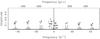 |
Fig. 1 Spectral window of the short-run CoRoT dataset of HD 174966. fs is the orbital frequency of the satellite. Amplitude in the ordinate axis is normalised to the highest peak. |
To avoid problems with power close to the zero frequency, the analysis with SigSpec was carried out in the range 0.05−100 d-1. In the case of Period04, the amplitude signal-to-noise ratio (S/N) 4.0 is the limit commonly used to consider a frequency as significant. In the case of SigSpec, the parameter used for significance is “sig” (= spectral significance), and the default limit is sig = 5.0. This is equivalent to about S/N = 3.8 (and sig = 5.46 is approximately equivalent to S/N = 4.0; Reegen 2007; Kallinger et al. 2008). However, we used a much more conservative limit, namely sig = 10.0, because the corresponding S/N values, determined using Period04 on the residuals, were much lower than expected2. This is probably caused by a high number of peaks still remaining among the residuals in the region of interest. This was explained in much more detail in similar recent works for other CoRoT targets: HD 50844 (Poretti et al. 2009), HD 49434 (Chapellier et al. 2011), and HD 50870 (Mantegazza et al. 2012).
The limit of sig = 10 was achieved after removing 185 peaks. This corresponded to a level of about 8 ppm for the smallest amplitudes. Table 6 (only available at the CDS) lists the frequencies obtained along with the most relevant parameters. The S/N values were calculated using Period04 on the residual file provided by the SigSpec package. Each S/N value was calculated within a box of width 5 d-1 centred on the corresponding peak, as is usual for this parameter (Breger et al. 1993; Rodríguez et al. 2006). In addition, columns nine to eleven list the formal error bars for frequencies, amplitudes, and phases determined using the formulae by Montgomery & O’Donoghue (1999).
The last column of the table lists possible identifications of harmonics or combinations as well as some controversial peaks, which appeared closer than the frequency resolution to another peak with higher amplitude. The origin of these controversial peaks could be related to a non-precise pre-whitening of a frequency from the light curve, generating spurious detections in the following analysis of the residuals.
We investigated harmonics and combinations up to the third order between the main peaks within a range of ±0.010 d-1. This study was made taking into account only the first 12 main peaks of the list (F1 to F12), harmonics until the fifth for F1 to F4, and combinations considering the first, second, and third orders (i.e. AFa + BFb being A, B = [1,3]). The possibility of interactions with the satellite orbital frequency (assumed as fs = 13.972 d-1, FS in the table) was also studied for the first four main peaks (F1 to F4) and the four first harmonics of fs (fs to 4fs). We also studied the possibility of remaining peaks (residuals) corresponding to the sidelobes of the 1 d-1 alias around fs and its harmonics.
A total of 37 possible combinations and harmonics were detected. However, most of them seemed to be coincidences. We investigated how well a frequency matched its exact theoretical combination. If a frequency, say Fab, is the result of a non-linear interaction between two (or more) frequencies, e.g. Fa and Fb, then its value should be exactly (theoretically speaking) the linear combination of the parent frequencies: Fab = Fa+b ≡ AFa + BFb (Garrido & Rodriguez 1996). We used the uncertainties in the peak and in the parent frequencies to check whether a frequency could be a combination. If the difference between the frequency and its mathematical combination is greater than the sum of all errors3 within 1σ, i.e. | Fab − Fa + b| > σFab + σFa + b, then the probability of such a frequency being a combination is quite low. Finally, 25 frequencies fulfilled this condition, and 19 of them still could be discarded as combinations when a 2σ error instead was used in the operation. Therefore, only 12 peaks of the original 37 remained as possible combinations.
This result is quite different from the one obtained for the CoRoT target HD 174936 (GH09), where no combination frequencies were reliably identified among the main frequency peaks. In fact, when comparing the periodograms of HD 174966 and HD 174936 we see two main differences: HD 174966 shows only few high-amplitude peaks, with amplitudes higher than detected in HD 174936, and overall a smaller number of frequencies is detected (185 significant peaks versus 422 peaks for HD 174936).
The range of statistically significant detected frequencies for HD 174966 goes from some value close to zero up to about 77 d-1, i.e. 900 μHz (1 d-1 = 11.57 μHz). But the highest amplitude peaks are grouped around 25 d-1 (300 μHZ, see Fig. 2).
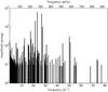 |
Fig. 2 Bar plot of the 185 frequencies extracted from the CoRoT light curve of HD 174966. The amplitude axis is in logarithmic scale and μmag units, and the frequency is shown in μHz and d-1 units. |
3. Spectroscopic analysis
3.1. Observations
The spectroscopic observations were performed between June 12, 2009 and August 5, 2009 (not contemporary with the CoRoT data). They covered a baseline of 53 days with 341 spectrograms and were performed with three different high-resolution spectrographs, as reported in Table 1.
Specifications of the spectroscopic observation.
The reduced spectrograms were brought to the same resolution of 65 000; then for each of them a mean profile was obtained by means of the least-squares deconvolution (LSD) technique (Donati et al. 1997) with values between −300 and +300 km s-1 with a 2 km s-1 step. We used the spectral region between 4140 and 5670 Å when calculating the LSD profiles, taking care to omit the regions containing hydrogen lines. The median S/N ratios of these profiles, as computed from the dispersion of their adjacent continua, are 5640, 1004, and 2945 for the HARPS, FOCES, and SOPHIE spectrograms, respectively.
The weighted average of the LSD profiles and its standard deviation are shown in the top and bottom panels, respectively, of Fig. 3. From the first three zeros of the FT of this average profile it has been possible to determine vsini = 126.1 ± 1.2 km s-1.
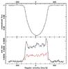 |
Fig. 3 Average of the LSD profiles (upper panel). Lower panel: root mean square (rms) standard deviation of the individual LSD profile with respect to the average one (black); residual standard deviation after the fit of the detected terms (red). |
3.2. Physical parameters
The Ground-Based Seismology Working Group (Catala et al. 2006) prepared the GAUDI archive4 (Solano et al. 2005) for the CoRoT mission, collecting high-resolution spectroscopy and multi-colour Strömgren photometry. The analysis of the uvbyβ photometry supplied the (preliminary) parameters: Teff = 7637 ± 200 K, log g = 4.03 ± 0.20 dex, and [Fe/H] = −0.11 ± 0.20 dex (Moon & Dworetsky 1985). They were very useful in the exploratory work for target selection, but the subsequent HARPS monitoring allowed us to perform a more accurate analysis.
The spectroscopic analysis was performed by using the set of HARPS spectra rather than the single spectrum taken with ELODIE at Observatoire Haute Provence available in the GAUDI archive. To this end, non-linear least-squares fits were performed on some regions of the very high S/N mean stellar spectrum by means of the sme code (Spectroscopy Made Easy, Valenti & Piskunov 1996). In particular, the regions around Hα, Hβ, Hγ, MgI 5180 triplet, 5300−5340 Å, and 4560−4795 Å were separately fitted. The Teff, log g, and [Fe/H] values thus obtained are listed in Table 2 with their internal errors. These HARPS values agree with those supplied by Strömgren photometry and with those from the ELODIE spectrum (both from the GAUDI archive) within the respective error bars.
The Teff = 7555 K value was used to compute the bolometric correction BC = 0.033 mag by means of the formulae given by Torres (2010). Strömgren photometry from GAUDI archive allowed us to determine the colour excess Eb − y and, in turn, the interstellar absorption AV = 0.025 mag. These corrections are very small with respect to the uncertainty on the Hipparcos parallax, 7.81 ± 0.66 mas (van Leeuwen 2007), from which Mbol = 2.16 ± 0.18 and L = 10.7 ± 1.7 L⊙ could be determined. From Mbol and Teff, a value of R = 1.90 ± 0.19 R⊙ can be obtained and, using the log g value, M = 2.16 ± 0.50 M⊙. This mass is higher than that calculated using the evolutionary tracks (M = 1.68 ± 0.1 M⊙; Schaller et al. 1992) and the uvby −Hβ calibration (M = 1.82 ± 0.09 M⊙; Ribas et al. 1997), but within the error bars derived from the calibration mean errors. We finally adopted the self-consistent values listed in Table 2 for the subsequent analysis of the line profile variations (LPV). A Hertzsprung-Russell (HR) diagram showing a model evolutionary track with those parameters adopted is plotted in Fig. 4. We also estimated that the fundamental radial mode frequency is 17.3 ± 2.5 d-1 (Eq. (6) in Breger 2000) and noted that this value is quite close to F5 = 17.62 d-1 in the CoRoT frequency list (Table 6).
Physical parameters of HD 174966.
Results of the mode identification from spectroscopic and Strömgren observations, as well as the values of n and ℓ obtained in the model fitting (last two columns).
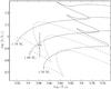 |
Fig. 4 HR diagram showing evolutionary tracks for 1.5, 1.6, and 1.7 M⊙. Models were computed using [Fe/H] = −0.08 dex, αML = 0.5, and dov = 0.2 from the pre-main sequence phase (dashed line) to the end of the main sequence (solid line). They included OPAL opacity tables and Eddington atmospheres. The position of HD 174966 and the spectroscopic 1σ uncertainty box derived in this work are also shown (see Table 2). |
Before proceeding to the mode identification, we derived the average line parameters by fitting the mean profile with the famias software (Zima 2008). We found a barycentric velocity of 9.1 ± 0.5 km s-1, an intrinsic line width of 8.1 ± 1 km s-1, and vsini = 126.2 ± 1.2 km s-1. The latter value is in perfect agreement with that obtained from the FT. Assuming R = 1.8 R⊙, this value corresponds to a break-up rotational velocity of 424 km s-1, which supplied the important constraint i > 17.5°.
3.3. Line profile variations
We analysed the LPV of the time series consisting of 341 LSD profiles using the pixel-by-pixel least-squares approach described by Mantegazza et al. (2000) and the pixel-by-pixel Fourier technique (Zima 2006). In the analysis we considered the part of the profile between −119 and +135 km s-1.
Among the detected terms there were three low-frequency ones (0.039, 0.253, and 0.472 d-1) and three high-frequency ones (46.96, 58.73, and 59.81 d-1). All these terms do not have photometric counterparts in the CoRoT lightcurve. Moreover, the behaviour of amplitude and phase curves across the line profile of the low-frequency terms is not easily interpretable in terms of pulsation modes; we suspect that they were introduced in the time series by the merging of data from three different instruments. The three high-frequency peaks have the appearance of low-degree retrograde modes. Taking into account their non-photometric detection, we suspect that they are aliases above the pseudo-Nyquist frequency of undetected lower frequency modes (in the range 20−40 d-1). Since we cannot be sure of their physical significance, we did not perform any mode identification for these six terms.
The mode identification was performed by means of the famias code. Table 3 lists the 18 detected modes in order of increasing frequency. The second column gives their amplitudes, in continuum units as defined in the famias software. These amplitudes are a measurement of the contribution of each term to the whole line profile variability. We report the S/N ratio, always as defined in famias, in the third column, and the best-fitting ℓ and m values in the fourth and fifth columns (negative m values correspond to retrograde modes).
Some of the spectroscopically detected modes have a photometric counterpart. In this case photometric frequencies and amplitudes are reported in the sixth and seventh columns. In particular, the frequency analysis of the LPV showed a distorted peak at the fourth photometric term (27.715 d-1). It is probably an unresolved bunch of peaks. We could tentatively disentangle it as a doublet composed of two modes at 27.720 and 27.709 d-1, but their values remain uncertain because they are at the limit of the spectroscopic resolution.
For each mode in Table 3, a best fit was performed on its amplitude and phase behaviours across the line profile, keeping as free parameters the velocity, the spherical degree, the azimuthal order, the amplitude, the phase, and the inclination. Then all the modes were fitted together, leaving for each of them the velocity amplitude as a free parameter and changing each time the inclination with a step of 5° from 20° to 90°. This enabled us to obtain a discriminant value for each inclination angle, i, by computing the differences between the observed and computed LPV, as described in Mantegazza (2000). The case of HD 174966 is less favourable than others (e.g. Mantegazza et al. 2000). Indeed, the behaviour of the discriminant shows a broad minimum centred at 62.5°, with very similar values in the interval from 45° to 70° (Fig. 5). For such an interval the stellar equatorial rotational velocities are within a well-constrained range, i.e. 135−178 km s-1. The corresponding rotational frequencies are in the 1.48−1.96 d-1 (17−23 μHz) range.
To proceed in our analysis we assumed i = 62.5°, v = 142 km s-1, and a rotational period of 0.64 d (rotational frequency 1.56 d-1 = 18.07 μHz), and we checked again the ℓ, m values of each mode. Only slight changes were found for some of them, all within the uncertainties of the ℓ, m determinations which are at least of the order of the unity (ℓ values are generally more reliable than m ones, especially for high m order modes). The uncertainties of ℓ,m values apply in particular to the close values of frequencies 23.152, 23.192, and 24.122 d-1, which are identified by famias with the same ℓ,m couple. This could also be due to the limited frequency resolution of the spectroscopic time series, which prevents us from obtaining clear amplitude and phase behaviours across the line profile in the case of close frequencies.
The case of the 6.8 d-1 component is interesting from a methodological point of view. Its phase curve across the line profile is typical for a high-degree prograde mode. However, this is very unlikely as 6.8 d-1 is much lower than the calculated fundamental radial frequency (17.3 ± 2.5 d-1, see Sect. 3.2). The frequency of retrograde modes is lower in the observer’s frame since they are travelling against the rotation. If the mode has a very high m order, the resulting frequency in the observer’s frame is negative, and we observe its mirrored peak in the positive plane. This could be the case for this component when considering m ~ −15 and the rotational frequency calculated above.
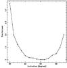 |
Fig. 5 Discriminant supplied by the simultaneous fit of all the identified modes versus the rotational axis inclination. |
4. Mode identification from Strömgren photometry
We obtained new multi-colour photometric observations for HD 174966 to perform a mode identification. The observations were made using the 0.9m telescope at Observatorio de Sierra Nevada (OSN), Spain, by means of a Strömgren six-channel simultaneous photometer (Nielsen 1983). A total of 953 points were collected in the four uvby bands simultaneously during 29 nights in 2007, between May 15 and August 23, and during seven nights in 2008, between July 1 and 11. To do the differential photometry, HD 173369 was selected as comparison star and HD 181414 as check star. Both stars are close to our object and, to date, they do not present any sign of variability in our ground-based observations.
Frequency analyses were carried out using the program Period04 (Lenz & Breger 2005). The values of the frequencies found in the light curves of the four bands were the same. The S/N reached in the v and b bands was higher than in the u and y bands. The u band is the noisiest (Martín & Rodríguez 2000). Table 4 shows the results of the amplitudes and phases for each frequency in the four bands. The values of the frequencies correspond to the highest amplitude frequencies detected in the CoRoT dataset.
Frequencies obtained from Strömgren photometry.
We used the amplitude and phase information of each frequency to identify the associated mode. The phase-shift versus amplitude-ratio diagrams (Garrido et al. 1990) allowed us to determine the spherical degree, ℓ. To that end, we computed non-rotating equilibrium and non-adiabatic oscillation models. We used the evolutionary code cesam (Morel 1997; Morel & Lebreton 2008) and the pulsation code graco (Moya et al. 2004; Moya & Garrido 2008) to calculate the equilibrium models and the non-adiabatic frequencies with ℓ = [0, 3], respectively. Computations included realistic atmosphere models (Kurucz 1993) to determine the non-adiabatic observables: φT, δTeff/Teff and δge/ge.
Non-adiabatic processes are sensitive to convection (Dupret et al. 2003; Daszyńska-Daszkiewicz et al. 2003; Moya et al. 2004). The larger the path travelled by a convective cell, i.e. the mixing length distance, the more heat is exchanged with its surroundings. We could then obtain information about the efficiency of the convection in HD 174966 through the free parameters αML of the mixing length theory and dov, where overshooting was used in every convection zone that appeared in the modelling, but not in the atmosphere. We used three values of each one in our computations: αML = 0.5, 1.0, and 1.5, and dov = 0.1, 0.2, and 0.3, and compared the theoretical non-adiabatic observables of the models with the phase-shifts and amplitude-ratios observed. A main result is that models with αML = 1.5 did not produce any phase-shift versus amplitude-ratio diagrams compatible with the observations. This inefficiency in the convection for δ Sct stars was previously pointed out by Daszyńska-Daszkiewicz et al. (2005); Casas et al. (2006, 2009). Other parameters, like metallicity, were also taken into account, but the results on the mode identification did not change.
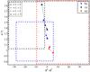 |
Fig. 6 Phase-shift versus amplitude-ratio diagram for the frequency of 21 d-1 and a non-rotating model with M = 1.55 M⊙, αML = 0.5, and dov = 0.2. Each box corresponds to a measure with its own uncertainties following the legend; band y is the reference. Every symbol (o, +, ∗, Δ) represents an ℓ degree (0, 1, 2, and 3, respectively). |
On the other hand, we are aware that multi-colour photometry identification predictions should be taken with care because rotation might have an influence on them (Daszyńska-Daszkiewicz et al. 2002). In particular, mode identification predictions depend on the inclination angle of the star and thereby on the rotation velocity (more exactly, on the deformation of the star caused by rotation). Here, the uncertainties in the colour indices together with the large range of most probable inclination angles (cf. Fig. 5) make angle-dependent identification predictions not feasible.
We illustrate the possible effect of rotation on the identification of modes using multi-colour photometry through the frequency that poses the most controversial mode identification, namely the frequency near 21 d-1. As illustrated in Fig. 6, the phase-shift versus amplitude-ratio diagram of this mode is quite peculiar. Band b indicates that all the ℓ values are possible, except ℓ = 3, whereas band v indicates the opposite.
In order to study the influence of rotation on the identification of that frequency, we
examined the behaviour of one of the largest effects on the frequency due to rotation, the
mode coupling or near degeneracy effects (see Soufi et al.
1998; Suárez et al. 2006b). We computed a
small grid of rotating models in the range of the physical parameters found in this work,
but varying the rotational velocity over the most probable values obtained from the
angle-discriminant figure (Fig. 5). Inclination values
of i ~ [35,80] degrees result in rotational velocities between 200
and 125 km s-1 when considering models used in this analysis. These velocities
imply ratios of Ωrot/Ωkep = 0.47 and 0.30 (with
 and Req being
the equatorial radius), respectively. This range of values can be considered still below
(but close to) the limit of validity of the perturbative approach, as stated by the test by
Suárez et al. (2005) and the comparison analysis
with the non-peturbative theory (see details in Sect. 5.1).
and Req being
the equatorial radius), respectively. This range of values can be considered still below
(but close to) the limit of validity of the perturbative approach, as stated by the test by
Suárez et al. (2005) and the comparison analysis
with the non-peturbative theory (see details in Sect. 5.1).
Asteroseismic rotating models were computed using the cesam code, taking first-order effects of rotation into account. This is done by including the spherically averaged contribution of the centrifugal acceleration, which is included by means of an effective gravity geff = g − Ac(r), where g is the local gravity, r is the radius, and Ac = 2/3rΩ2 is the centrifugal acceleration of matter elements. The non-spherical components of the centrifugal acceleration are included in the adiabatic oscillation computations (Suárez et al. 2006a). Adiabatic oscillations were computed using the adiabatic oscillation code filou (Suárez 2002; Suárez & Goupil 2008). This code provides theoretical adiabatic oscillations of a given equilibrium model corrected up to the second-order for the effects of rotation. These include near-degeneracy effects, which occur when two or more frequencies are close to each other. In addition, the perturbative description adopted takes radial variation of the angular velocity (radial differential rotation) into account in the oscillation equations.
We constrained the models to those fitting the frequency at ~21 d-1 within a frequency uncertainty up to the Rayleigh frequency. We used a heuristic method based on the best frequency fitting. In this method, we considered as best models those with the lowest values of the χ2 distribution.
All the best models except for one found the mode as non-coupled with values of (n,ℓ,m) = (1, 2, −1) or (0,3,2). Only the model with also the lowest χ2 showed that the frequency could be a coupling between the modes (1,1,0) and (−1,3,0). In any case, the interesting point here is the value of the rotation for the best models rather than the identification itself. Due to the methodology, both the rotation values and the identification are products of the heuristic but do not interfere with each other.
The best models show rotational velocities around 200 and 130 km s-1, which correspond to the extremes of the most probable range of inclination angles, i.e. 35 and 76 degrees, respectively. In order to find models with i close to the 62.5 degrees (the minimum of the angle discriminant in Fig. 5), we had to relax the criteria of Teff, log g from the spectroscopic uncertainty box to the photometric one (see Sect. 3.2) and frequency match error (for 21 d-1) to twice the Rayleigh frequency. In short, the variation of the inclination angle here does not affect the predictions of the rotating models for that frequency.
The results on the identification are shown in Table 3. The compatible values of the spherical degree for each frequency are listed in the column ℓ. The ambiguity of the 21 d-1 mode is not clarified by the rotating model study, which identifies that frequency as an ℓ = 2 or 3 multiplet or a possible coupled mode, in contrast to the spectroscopic results, which predict an ℓ = 1 mode. Nonetheless, the spectroscopic identification does not take high rotation into account, i.e. the star is considered spherical. This is solved in our perturbative approach for the oscillation frequencies, which takes into account the deformation of the star due to rotation. In any case, the mode identification explained here must be taken carefully since the perturbative approach is close to the limit of validity for HD 174966 (see Sect. 5.1).
5. Best-fitting model
We used the information of the physical parameters and the mode identification derived in this work to search for the best representative models of HD 174966, i.e. those that fulfil all the constraints derived from the observations. A new and denser grid of non-rotating models were computed to this aim.
We computed the range [1.25, 2.20] M⊙ in mass with a step of 0.01 and the range [−0.52, 0.08] dex in [Fe/H] with a step of 0.2, covering the whole δ Sct instability strip. We used the same codes as in the previous section: cesam and graco for the main-sequence non-rotating equilibrium and oscillation models respectively. Again, non-adiabatic frequencies were computed. The models included Eddington atmospheres and the same values for the convective parameters αML (0.5, 1.0, and 1.5) and dov (0.1, 0.2, and 0.3). We only considered the range of ℓ = [0, 3], because the visibility of the modes in the integrated light decreases with the spherical degree (Dziembowski 1977). The frequencies with the highest amplitudes in the CoRoT observations will be mainly low-order modes, so the range of computed ℓ’s must be enough to describe them.
Around 500 000 models were computed. This grid includes all the models lying in the HD 174966 uncertainty box (1σ) obtained from the spectroscopic observations. To efficiently handle this large number of models, we took advantage of VOTA (Virtual Observatory Tool for Asteroseismology, Suárez et al. 2013), a tool designed to easily handle stellar and seismic models, analyse their properties, compare them with observational data, and find models representative of the studied stars.
We then selected the models fulfilling the spectroscopic 1σ uncertainty
box determined in this work. A total of 426 models fulfilled
Teff, log g and [Fe/H], which led to the
following physical parameters: M = [1.49, 1.58]
M⊙, R = [1.50, 1.73]
R⊙, L = [6.47, 8.92]
L⊙,  = [0.43, 0.62] g cm-3, and age = [826, 1306] Myr. The value of −0.12 in
metallicity of our grid is the only one compatible with the spectroscopic observations.
= [0.43, 0.62] g cm-3, and age = [826, 1306] Myr. The value of −0.12 in
metallicity of our grid is the only one compatible with the spectroscopic observations.
Finally, we applied the results to the mode identification. This included the discriminant obtained from the photometric observations about the convective efficiency: α ≠ 1.5. The frequencies used for the discrimination in the models were 18.131, 23.152, 23.192, 24.122, and 26.955 d-1 (209.85, 267.96, 268.43, 279.19, and 311.98 μHz, respectively). These frequencies were selected because their mode identification is the only that could be compared with the computed modes of our grid of non-rotating models, i.e. these frequencies have ℓ ≤ 3 modes and m = −1 or 15. The frequency at ~21 d-1 was not used because of its possibly coupled nature.
To fit models, all the possibilities in the spherical degree (limited by the error bars and
up to ℓ = 3) were taken into account as valid solutions6. The result is that 21 models fulfilled all the constraints, giving
the same values for the (n, ℓ) pairs (see last two columns
in Table 3). The characteristics of the models are
Teff = [7510, 7592] K, log g = [4.17, 4.19]
dex, R = [1.64, 1.69] R⊙, M =
[1.53, 1.56] M⊙, L = [7.82, 8.37]
L⊙,
= [0.455, 0.487] g cm-3, age = [1046, 1186] Myrs, [Fe/H] = −0.12 dex,
Xc = [0.4398, 0.4767], αML = [0.5,
1.0], dov = [0.1, 0.2]. The values for the mass and the radius
are lower than those found in the spectroscopic analysis, although still within the
uncertainties. This could be due to the slightly lower metallicity of our models. In
addition, the limitation of using only the frequencies as m = 0 modes is a
source of inaccuracy.
5.1. Influence of rotation
The methods to determine physical parameters, identify the modes, and calculate models presented in the previous sections do not properly account for rotational effects. In the determination of the physical parameters, the rotational effects are taken into account through dividing the star into annular regions, each characterised by a single intensity spectrum, and reducing the flux spectrum to a one-dimensional sum (Valenti & Piskunov 1996). Therefore, rotational velocity is well determined but only as a maximum projected value (differential rotation also has an effect in the determination of the other observables). However, the resulting quantities of the effective temperature and surface gravity are a mean value of the integration of the stellar disk. For rapidly rotating stars, such a value for describing the whole body is not reliable. Due to the flattening produced by rotation, these quantities differ from the pole to the equator. In that way, the formal errors derived from fitting the spectra are too small.
The mode identification efforts are less accurate. For δ Sct stars, the problem usually lies in the low number of frequencies observed from the ground, the unknown of the physical processes involved in the selection mechanisms and the usually rapid rotation of these objects. The latter is the most complicated task to resolve because even the perturbative methods reach their limit of validity to describe pulsations for typical rotational velocities of δ Sct stars. In recent years, some works have shed light on this problem, thanks to the full integration of the oscillation equations in 2D models (see, for example, Lignières et al. 2006; Reese et al. 2006). The computations showed how the modes reach a new distribution within the oblate star.
This could impact spectroscopic line variations used in mode identification. The famias code uses the Fourier parameter fit method (Zima 2006) and the moment method (Balona 1986a,b, 1987; Briquet & Aerts 2003) to carry out a mode identification. Both methods assume oscillations in the limit of linearity (sinusoidal variations) and slow rotation (neglecting second-order rotational effects), questioning the obtainment of a reliable mode identification for moderate-to-rapidly rotating stars. Consequently, the mode identification acquired in this work may be incorrect for some modes: those most affected by rotation. It is not possible to identify which frequencies are poorly detected with the tools and methods developed to date.
Rotation effects are also non-negligible in multi-colour photometry, as discussed in Sect. 4. In this case, the value of the inclination angle of the star affects φT, δTeff/Teff, and δge/ge. This implies a dependency of the amplitude-ratios and phase-differences on the azimuthal order (Daszyńska-Daszkiewicz et al. 2002; Casas et al. 2006). Pertubative methods are able to compute these implications for moderately rotating stars, but the extreme cases require a special treatment. Reese et al. (2012), using their code to fully integrate the oscillating modes, have presented a method to compute amplitude-ratios in the Geneva photometric system. Although this is a promising result, their computations did not include non-adiabatic effects, which are essential for a true determination of the frequencies’ amplitudes.
In addition, the star is no longer spherical and some quantities, like the radius, might not be determined with the direct comparison to 1D non-rotating models (the equatorial radius is different from the polar radius). These facts introduce a strong uncertainty and inaccuracy in the physical characteristics derived for HD 174966 in the previous sections.
Despite these problems, the non-perturbative computations have shown that some structures, like the large separation and the rotational splitting, are still identifiable in the frequency distribution (Lignières et al. 2006, 2010). This is the reason for searching for patterns and structures within the periodogram of HD 174966.
6. Quasiperiodic patterns within the frequency spectrum
To search for periodicities in the frequency set of HD 174966, we used the same Fourier
analysis as in GH09. An ideal periodic pattern is represented as a series of equally spaced
Dirac deltas, i.e. a Dirac comb. The FT of a Dirac comb is another Dirac comb with inverse
periodicity of the original one. So, the more the FT resembles a Dirac comb, the more
confident we are that the frequency spectrum has a periodicity. A realistic case can be
represented as a Dirac comb, if our function is periodic, multiplied by a rectangular
function (because the number of frequencies is finite): 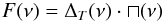 (1)where
ΔT(ν) is the Dirac comb function with a
periodicity of T and ⊓ (ν) is the rectangular function.
Then, the FT is:
(1)where
ΔT(ν) is the Dirac comb function with a
periodicity of T and ⊓ (ν) is the rectangular function.
Then, the FT is: 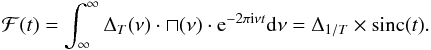 (2)Due to the rectangular function, the form of
the FT is not a perfect Dirac comb but a convolution with a sinc function. The side lobes
originated by the sinc function hinder the identification of the periodicity. In addition,
other characteristics of a true frequency spectrum make the identification difficult. A
pattern with an inexact periodicity (quasiperiodic), where frequencies do not belong to the
pattern or some values are missing, would produce broadened peaks, spurious peaks (“noise”
in the FT), and less powerful sub-multiples.
(2)Due to the rectangular function, the form of
the FT is not a perfect Dirac comb but a convolution with a sinc function. The side lobes
originated by the sinc function hinder the identification of the periodicity. In addition,
other characteristics of a true frequency spectrum make the identification difficult. A
pattern with an inexact periodicity (quasiperiodic), where frequencies do not belong to the
pattern or some values are missing, would produce broadened peaks, spurious peaks (“noise”
in the FT), and less powerful sub-multiples.
We applied the method to the frequency spectrum of HD 174966. In our calculations, we neglected the amplitudes of the frequencies to avoid biases coming from the unknown mode selection. The resulting FT is given in Fig. 7. We selected subsets of frequencies, namely subsets with the 30, 60, 112 highest frequencies, and a subset including all of them, for which we did not include the close peaks. Each subsequent subset contains the previous one. The main assumption we made is that the periodicity is due to frequencies with low ℓ. The visibility of the modes decreases approximately as ℓ-2.5 or ℓ-3.5, depending whether the ℓ degree is odd or even (Dziembowski 1977). This assumption is supported by the LPV analysis (see Sect. 3.3), despite the possible inaccuracy of the mode identification method. The periodicity appears, above all, in the FTs of the subsets including a relatively low number of frequencies (30 and 60). We calculated the FT and presented the result in frequency scale to obtain a value of the periodicity in μHz (and d-1).
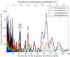 |
Fig. 7 Fourier transform of various subsets selected by amplitude. The blue, green, red, and cyan lines correspond to the FT calculated from the subset including the first 30, 60, 112, and 168 (all the peaks except the close ones) highest amplitude frequencies, respectively. The peaks corresponding to the large separation (64 μHz) and its sub-multiples are labelled (see text). |
We identify a peak as the periodicity of a pattern when the value and its sub-multiples7 are found. As illustrated in Fig. 7, we identified a pattern with a periodicity of 64 μHz (5.53 d-1) in the frequency set. Any of the peaks we used to detect a pattern do not disappear when the number of frequencies involved in the FT is increased. Even when we do not use the 12 peaks that might be combinations, the value of the periodicity does not change appreciably. These facts ensure that the pattern is real.
6.1. Large separation or rotational splitting structure?
The main question rising from the result in the previous section is the origin of the periodic pattern. Usually, the presence of a periodicity has been associated with the so-called large separation structure, which is common in frequencies that have reached the asymptotic regime, like those in the solar-type pulsators. However, it is not expected to appear in the regime where the δ Sct stars pulsations locate.
GH09 proposed that the origin of the periodicity could be linked to the large separation,usually defined as: Δνℓ = νn + 1,ℓ − νn,ℓ, although out of the asymptotic regime. Figure 4 of GH09 showed a plot of νn,ℓ versus Δν for a non-rotating model: Δν increases with frequency within the typical range of observed frequencies in δ Sct stars, ν ≤ 1000 μHz. However, within the interval [100, 600] μHz (which depends on the physical characteristics of the star and on the age), Δν comes to a halt and most of its values are confined within less than 4 μHz. Although it is not a constant function, the range of variation is small enough to consider it as a roughly quasiperiodic regime and the FT would be able to detect it.
On the other hand, the origin of the periodic pattern has been also associated with the rotational splitting, which, for low rotation rates, forms multiplets with a periodicity equal to the rotational velocity. However, for large rotation values, multiplets become irregular (see Soufi et al. 1995; Suárez et al. 2006a), breaking the periodic structure. Nonetheless, in a recent work, Lignières et al. (2010) searched for patterns within the frequency set computed with the non-perturbative method. To do that, they considered a visibility function for the computed frequency set and calculated its autocorrelation. For some configurations of the inclination angle of the stellar rotational axis, they found a peak in the autocorrelation function corresponding to twice the rotational splitting frequency.
To differentiate between a periodic pattern coming from a large separation structure or from the rotational splitting, we have to analyse the case of HD 174966 carefully. First, we have to note that the FT, as it is defined, is more sensitive to periodicities rather than other kind of spacings, such as a preferred randomly distributed frequency difference. In the asymptotic regime, the large separation has a comb structure and should be easily discovered with the FT. The large separation structure is even conserved with high rotational velocities because the structure is led by the so-called island modes (the new distribution that appears when non-perturbative theory is applied to pulsation in fast rotators, Lignières et al. 2006).
Concerning rotational splitting for the high-velocity regime, modes containing the rotational information are the so-called chaotic modes. They are irregularly distributed in the frequency spectrum, as the results of the studies based on ray mechanics formalism showed (Lignières et al. 2006). One should not expect to find regular patterns in it. Despite that, the modes have specific statistical properties, which can be detected with an autocorrelation function. This is the case of the 2Ω pattern showed in Lignières et al. (2010), a randomly distributed frequency difference, which is, however, hardly identifiable using an FT.
In addition, using the physical parameters derived in the spectroscopic analysis for HD 174966, the rotational splitting should be 18.07 μHz. Twice this value is only half of that found in the observed frequency set (64 μHz). But even taking into account the uncertainties about the determination of the inclination angle (i.e. discriminant value ±0.02) and the worst favourable case for the radius of the star that we derived from the models, the rotational splitting would be, at the most, ~29 μHz.
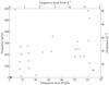 |
Fig. 8 Echelle diagram for the 30 frequencies of highest amplitude of the HD 174966 frequency spectrum using a periodicity of 65 μHz. |
All this led us to think that the pattern found in HD 174966 is a consequence of the large separation. However, in order to define definitively the structure of the pattern, we constructed an Echelle diagram, which can be seen in Fig. 8. In this plot, the 30 frequencies of highest amplitude of the HD 174966 spectrum have been used because they contain the information of the periodicity; in addition, a spacing of 65 μHz has been used. The frequencies involved in the pattern are clearly differentiated. Indeed, there are two groups of frequencies, placed at the left of the plot, which have an almost identical structure to the solar-like stars case. The main difference is the range in which the pattern appears, far from the asymptotic regime but around the fundamental radial mode value.
There is no doubt that the frequency periodic pattern (indeed, two patterns) for this object comes from a large separation-like structure. The question now is whether it is possible to extract some information related to the interior of the star using this periodicity.
7. The large separation as an observable
There exists a previous attempt to use the large separation in δ Sct stars as an observable. Breger et al. (2009) used a histogram of differences to search for periodicities. They found a periodic pattern in three δ Sct stars and systematized a method to reduce the uncertainties on the determination of the physical parameters. However, their method had two main problems. First, the frequency of the lowest unstable radial mode had to be identified. This corresponded to a frequency within the cluster of modes at the lowest frequencies detected from the ground. It was a cluster because of the assumption of trapped modes. But space observations of δ Sct stars showed that in many cases it was difficult to identify a cluster with the lowest frequency, as can be seen in Fig. 2 and with HD 174936 (GH09). Second, they took into account only the radial modes. As shown in Fig. 4 on GH09, the periodicity in non-rotating models and in models with rapid rotation (Lignières et al. 2006) is not only formed by the modes with ℓ = 0. Even more, the large separation is better defined by the non-radial ones (until the avoided-crossing effects appear).
The aim of this work is to use the large separation found in the previous sections combined with that present in the non-rotating models to obtain some information about the internal structure of the star. This method is supported by the fact that, although the value of the frequencies globally decreases when rotation increases and, so, the large separation, Δν is reasonably conserved up to Ω/ΩK ~ 0.4 (F. Lignières & D. Reese, priv. comm.). Because HD 174966 rotates around or below this limit, we can suppose that the difference in the large separation between the rotating and non-rotating case is included in the error bars of Δν.
In Fig. 9, we applied the FT to the frequencies below 600 μHz (to match the observations) of a non-rotating model representative of the star, i.e. fulfilling the spectroscopic physical parameters. A similar structure to that found in the observations can be seen, with the main peak plus the sub-multiples, resulting in a periodicity of ~67 μHz. Following this procedure, the models and the observations are directly comparable.
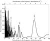 |
Fig. 9 Fourier transform, as explained in Sect. 6, of a non-rotating model (M = 1.55 M⊙, [Fe/H] = −0.12, αML = 0.5, and dov = 0.2) representative of HD 174966. A periodicity of ~67 μHz is clearly identifiable. The FT was computed using only frequencies below 600 μHz (51.84 d-1). |
However, not all the physical quantities obtained from this comparison are reliable. As discussed in Sect. 5.1, the physical parameters could differ from the slow-rotation case to the fast-rotation one. Fortunately, the work by Reese et al. (2008) suggested that the large separation for the case of rapid rotators is still related in a simple way to the mean density of the star. Even more, it suggested that the large separation to mean density ratio is roughly constant for all the rotation rates they computed. These results gave us the opportunity to determine the mean density of HD 174966 using our grid of non-rotating models, even when the other quantities, such as the radius or the mass, could not be completely trusted.
As a starting point, we adopted the parameters Teff, log g, and [Fe/H] from the spectroscopic analysis: Teff = 7555 ± 50 K, log g = 4.21 ± 0.05 dex, and [Fe/H] = −0.08 ± 0.10 dex (cf. Sect. 3.2). We used the non-rotating models of our grid covering the entire 1σ uncertainty box and looked for those with the same Δν (in the δ Sct pulsation regime) as that found in the observations. For simplicity, in the models a mean value of Δν is calculated using only p modes because the large separation is a property of the acoustic modes. In addition, we used the modes within the observed range (until n = 8) to be consistent with the observations. The observed Δν value was taken as an average of the frequency differences from the two columns that form the large separation pattern in the Echelle diagram (Fig. 8). Hence, Δν = 65 ± 1 μHz, with the uncertainty being the standard deviation.
For comparison, Table 5 summarizes the range in the physical parameters achieved by the classical methods (photometric and spectroscopic determination of Teff, log g, and [Fe/H]) and adds the use of the large separation. We also included the result obtained in the multi-colour analysis: αML ≤ 1.0. As can be seen, with the large separation we obtained a precision in the mass, radius, surface gravity, and, above all, in the density of the star that has never reached before. As previously discussed, the results in the radius and mass should be taken with care. It is important to note that the large separation could not reduce the uncertainty in Teff. In addition, the uncertainties are a bit constrained by the fact that our grid did not scan enough of the space defined by the physical parameters (steps were too large).
Table summarizing the range of validity of the physical quantities of HD 174966 obtained using the different methods discussed in this work.
The most important advantage of the method described above is that no assumption about the rotation of the star is needed to derive an accurate value of the mean density (e.g. a fundamental quantity in the characterisation of a planetary system). The main assumption was about the visibility of the oscillation modes and physical parameters taken as starting point in the analysis.
In the work we present here, we have used the values of the high-quality spectroscopic
measurements, obtaining a value for
with an uncertainty of 6%. Nonetheless, even if the parameters from the photometry were used
instead and no information about the Strömgren photometry was used, i.e. about the
non-validity of αML = 1.5, the resulting mean density would be
of
= [0.48, 0.59] g cm-3. This is a major improvement because we obtain a better
measurement of the mean density of the star than that achieved by any spectroscopic
observation.
7.1. Towards a reliable mode identification using the periodicity
At this point we wondered if it is possible to extract more information from the large separation pattern. Thanks to the Echelle diagram, mode identification is feasible in solar-like stars, using the structure of the pattern and its well-known distribution with the spherical degree. A direct comparison between one of these diagrams for the model and for the observation gives a direct identification of ℓ. While this is a consequence of the asymptotic regime, it is not the case for δ Sct stars. Figure 8 shows that the frequencies comprising the two columns pattern are below 300 μHz. Plotting an Echelle diagram for our non-rotating models did not give this structure. It only gave a straight distribution for some modes, which form the large separation comb used in the previous section.
We moved to our grid of rotating models, searching for a representative one of HD 174966. Following the same procedure of selecting models fulfilling the spectroscopic parameters, we selected then those with a large separation within the uncertainties derived in the previous section (65 ± 1 μHz). The large separation, in this case, was calculated as an average value of the frequencies with ℓ = 1 up to n = 8 in order to match the observations (frequency range below ~600 μHz). The ℓ = 1 modes are the best determined in the second-order perturbative approximation compared to the values computed with non-perturbative methods (Lignières et al. 2006). This indicates that some reliable conclusions can be obtained from the distribution of the spherical degrees observing our rotating models.
The six final models selected cover the uncertainty range of the inclination angle, meaning rotational velocities from ~125 km s-1 up to ~200 km s-1. Coherent with the predictions by Reese et al. (2008), the mean density of these models discriminated by large separation is [0.54, 0.58] g cm-3, which is in the same range as for the non-rotating ones (see Table 5). The masses, however, vary from 1.55 M⊙ to 1.61 M⊙, slightly higher than that obtained in the previous section.
We applied the FT procedure to the models to find a periodicity and used it to construct an Echelle diagram. An example can be seen in Fig. 10. We only used the lowest spherical degrees (ℓ = 0, 1), assuming the same visibility of the mode as in Sect. 6, and frequencies below 500 μHz to select the range of the observed Echelle. All the plots showed the same structure: the ℓ = 0 modes aligned with the ℓ = 1, but only with m = −1 and m = 1, and the ℓ = 1, m = 0 modes form another structure (indeed, also becoming a pattern, but with a slightly higher periodicity, typically ~5 μHz more). The difference between the azimuthal orders m = −1 and m = 1 appeared to be independent from the model, although the m = 0 values showed a displacement with rotation. The most different behaviour was found in the model with the highest rotational velocity.
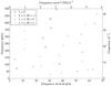 |
Fig. 10 Echelle diagram for a 1.61 M⊙ rotating model of HD 174966, with ~135 km s-1. Each couple (ℓ = 0; ℓ = 1,m = −1; ℓ = 1,m = 0; ℓ = 1,m = 1) is depicted with a different colour (black, blue, red, and green, respectively) and a symbol (◯, □, ×, and ▵, respectively). A structure similar to the large separation found in the observations can be seen for some of these pairs between 200−350 μHz. This structure is mainly formed by the ℓ = 1 modes. |
It is not feasible to say that we are able to do a mode identification using these models or even to say that the observed patterns are ℓ = 1 modes. Although the pattern is seen in the models, it is clear that some gaps exist between the observations and the theory. First, the columns in the Echelle diagram of the CoRoT frequencies are closer than any pair of combs in the models. Second, the frequencies in the observations are more tightly distributed. Finally, the lowest frequencies in the pattern of the observations lie below 100 μHz, which is lower than the values of the patterns in the models.
Maybe these differences could be explained because frequencies at high rotation rates tend to decrease with respect to their non-rotating values (Lignières et al. 2006). Nonetheless, this range below 100 μHz typically corresponds to g modes. No recent works related to pulsations in highly rotating stars showed the combined analysis of the pressure and gravity modes. It seems, looking at the observations, that a new regime is also reached at these velocities around the fundamental radial mode. It could be useful to note that at 30% of the Keplerian limit an interesting reorganisation of p modes occurs (Fig. 4 in Reese et al. 2006). It is not an exaggeration to think that this might be the case but with the additional effect in the g modes. This study has not yet been made; therefore, a mode identification is not possible at this point.
Regardless of this last conclusion, searching for structures within the frequency spectra of δ Sct stars seems to be one of the best ways to finally achieve a full understanding of the interior of this complex type of pulsators. The recent development of the non-perturbative theory is also needed. However, because computations are up to now highly time consuming, the comparison with non-rotating models, as shown in this work, could be the way to characterise a large sample of A-F type stars, such as those provided by the Kepler satellite.
8. Conclusions
In the present work, we used the most advanced methodology available to study the δ Sct star HD 174966. In particular, we analysed the CoRoT light curve and performed new high-resolution spectroscopic and multi-colour photometric ground-based observations. We carried out an in-depth study of this pulsator, comparing the result from every single method and using all the information to try to derive the most accurate physical parameters of its interior.
From the CoRoT light curve, we extracted 185 frequencies above the limit of sig = 10 within the range from a value close to zero up to about 77 d-1, i.e. 900 μHz. This limit translates to 8 ppm for the smallest peak. We found that 17 of these peaks were located closer than the limit resolution to others. In addition, 37 more peaks were identified as possible combinations, although 25 of them seemed to be only coincidences. In summary, 158 peaks could be considered as independent frequencies. This number is significantly smaller than previous δ Sct stars observed by CoRoT, but we have to take into account the shorter time baseline.
From the spectroscopic observations, we derived the physical parameters, including the inclination angle and rotational velocity. We extracted 18 frequencies and performed a mode identification. Most of them corresponded to the modes extracted from the CoRoT light curve, and one appeared to be a double peak not resolved in the CoRoT frequency set.
In addition, the three highest peaks of the 158 CoRoT frequencies were also detected from ground-based uvby photometry. The mode identification from multi-colour photometry is in good agreement with that from high-resolution spectroscopy. For the lowest amplitude peak we found a discrepancy, whose detailed analysis using rotating models indicated an ℓ = 2 or 3 non-coupled mode or a coupling between modes ℓ = 1 and 3, in contrast with the spectroscopic value, ℓ = 1. Another important result concerns the αML parameter of the convention theory: αML< 1.5, which is lower than that usually used for intermediate-mass stars.
We tried to constrain the modelling of the star using the information from the proposed mode identification. Twenty one models were found to fulfil all the constraints, and their physical parameters were slightly lower than those found in the spectroscopic analysis, although within the uncertainties. Nevertheless, these results might not be very accurate because, for instance, models did not account properly for fast rotation. In particular, we need non-perturbative models that properly include the rotational effects, although they are very time consuming. On the other hand, the fast rotation amplifies the differences between stellar and observer frames. Two modes with different m could be unresolved in the observer reference frame. In such a case it could be very difficult to correctly decipher the resulting amplitude and phase diagrams and provide a reliable mode identification. In addition, the LPV method neglects the second-order rotational effects, so it is not prepared to describe the new order of the modes showed by non-perturbative computations. These facts make difficult the comparison between theory and observations and, consequently, the extraction of accurate information about the stellar interior.
As in previous cases (HD 174936, GH09, and HD 50870, Mantegazza et al. 2012), we searched for periodic patterns within the frequency
set of HD 174966, expecting that a relative measurement could be used to infer useful
information from the spectrum. We found a periodicity of ~64 μHz (5.53
d-1). Thanks to the estimate of the inclination angle obtained from the
analysis of the LPV and an Echelle diagram clearly showing a structure, we were able to
discard the rotational origin of the pattern and identify it as a large separation. We
studied the possibility of using Δν as an observable, discriminating
non-rotating models of a grid with the objective of reducing the uncertainty in the mean
density of the star. Through the Echelle diagram, a tight value of the large separation was
obtained: Δν = 65 ± 1μHz. Using this value, we found that
= [0.51, 0.57] g cm-3, which supposes an uncertainty of 6%, never reached before
for a non-binary δ Sct star. The main advantage of this method is that no
initial assumptions related to the rotation are needed to find the periodicity from the
observations because its value depends only slightly on the velocity of the star.
Moreover, comparing the observed Echelle diagram to other rotating models computed using second-order terms in the perturbative theory, we found a similar structure of the large separation, formed mainly by the ℓ = 1 modes with m = –1, 1. The pattern observed also seems to include some gravity modes, which was unexpected and never described in the literature. Nonetheless, although the models could not be used in this case to perform a mode identification, we showed that it might be feasible using the new modelling techniques and that the large separation pattern is a useful tool in this task even for δ Sct stars. Further investigations on the Echelle diagrams of theoretical models should be done to elucidate the organisation observed in the pulsating modes.
All these results demonstrate the usefulness of the large separation in δ Sct stars. This separation will allow the determination of the mean density of one object with this kind of pulsation, regardless of its rotational velocity (this assertion will have to be confirmed for every rotation rate). This is an affordable method for the precise study of δ Sct pulsators and a major improvement in the study and characterisation of, for example, planetary systems hosting A-F type stars.
Essentially, points flagged by the reduction pipeline: hot pixels detected, the passing through the South Atlantic Anomaly (SAA), interpolated points, etc.
The S/N obtained on the residuals for a sig = 5.0 was lower than the expected value S/N = 3.8. We used the limit sig = 10.0 to ensure that we are above the usual limit of S/N = 4.0.
To derive uncertainties in the determination of mathematical combinations, we follow the standard theory on error propagation: | σFa + b| = |A·σFa| + |B·σFb |. Because no information about the uncertainty in the satellite orbital frequency is available, it was treated as a constant in our calculations.
None of the frequencies was identified as m = 0 in the LPV analysis, which is the only value compatible with non-rotating models. However, m = 0 is valid for the selected frequencies within the ± 1 uncertainty.
For example, for the 23.192 d-1 frequency, we searched the closest mode with the possible ℓ = [0, 1, 2].
The periodicity of the Dirac comb resulting from the FT is k/T, where k is an integer. In the inverse scale of the plot, we will see T/k.
Acknowledgments
The authors thank the anonymous referee for useful comments, which allowed them to improve the paper. The authors wish to thank L. Mantegazza for having performed important parts of the spectroscopic analysis. The authors wish to thank John Telting for useful comments on an advanced draft of the paper. A.G.H. wishes to thank S. Murphy for his careful revision of the text. A.G.H. was supported by grant BES2005-8478, under the project “Participación española en la misión CoRoT” (ESP2004-3855-C03-01) and is supported by grant SFRH/BPD/80619/2011 from FCT (Portugal). A.G.H. acknowledges financial support from project PTDC/CTE-AST/098754/2008 from FCT (Portugal). A.M. acknowledges funding by AstroMadrid (CAM S2009/ESP-1496) and the Spanish grants ESP2007-65475-C02-02, AYA 2010-21161-C02-02. J.C.S. acknowledges support by the Spanish National Research Plan (grants ESP2010-20982-C02-01, AYA2010-12030-E). M.R. and E.P. acknowledge financial support from the Italian PRIN-INAF 2010 Asteroseismology: looking inside the stars with space- and ground-based observations. P.J.A. acknowledges financial support from grant AYA2010-14840 of the previous Spanish Ministry of Science and Innovation (MICINN), currently Ministry of Economy and Competitiveness. K.U. acknowledges financial support by the Spanish National Plan of R&D for 2010, project AYA2010-17803. E.S. and C.R. acknowledge support from the Spanish Virtual Observatory financed by the Spanish MICINN and MINECO through grants AyA2008-02156 and AyA2011-24052. This work was supported by GRID-CSIC Project (200450E494). This research benefited from the computing resources provided by the European Grid Infrastructure (EGI). This investigation was partially supported by the Junta de Andalucía and the Spanish Dirección General de Investigación (DGI) under project AYA2009-10394.
References
- Auvergne, M., Bodin, P., Boisnard, L., et al. 2009, A&A, 506, 411 [NASA ADS] [CrossRef] [EDP Sciences] [Google Scholar]
- Baglin, A., Auvergne, M., Barge, P., et al. 2006, in ESA SP, 1306, eds. M. Fridlund, A. Baglin, J. Lochard, & L. Conroy, 33 [Google Scholar]
- Balona, L. A. 1986a, MNRAS, 219, 111 [Google Scholar]
- Balona, L. A. 1986b, MNRAS, 220, 647 [NASA ADS] [CrossRef] [Google Scholar]
- Balona, L. A. 1987, MNRAS, 224, 41 [NASA ADS] [CrossRef] [Google Scholar]
- Balona, L. A., & Dziembowski, W. A. 2011, MNRAS, 417, 591 [NASA ADS] [CrossRef] [Google Scholar]
- Borucki, W. J., Koch, D., Basri, G., et al. 2010, Science, 327, 977 [NASA ADS] [CrossRef] [PubMed] [Google Scholar]
- Breger, M. 2000, in Delta Scuti and Related Stars, Reference Handbook and Proceedings of the 6th Vienna Workshop in Astrophysics, eds. M. Breger, & M. Montgomery (San Francisco: ASP), ASP Conf. Ser., 210, 3 [Google Scholar]
- Breger, M., Stich, J., Garrido, R., et al. 1993, A&A, 271, 482 [NASA ADS] [Google Scholar]
- Breger, M., Pamyatnykh, A. A., Pikall, H., & Garrido, R. 1999, A&A, 341, 151 [NASA ADS] [Google Scholar]
- Breger, M., Lenz, P., Antoci, V., et al. 2005, A&A, 435, 955 [NASA ADS] [CrossRef] [EDP Sciences] [Google Scholar]
- Breger, M., Lenz, P., & Pamyatnykh, A. A. 2009, MNRAS, 396, 291 [NASA ADS] [CrossRef] [Google Scholar]
- Briquet, M., & Aerts, C. 2003, A&A, 398, 687 [NASA ADS] [CrossRef] [EDP Sciences] [Google Scholar]
- Casas, R., Suárez, J. C., Moya, A., & Garrido, R. 2006, A&A, 455, 1019 [NASA ADS] [CrossRef] [EDP Sciences] [Google Scholar]
- Casas, R., Moya, A., Suárez, J. C., et al. 2009, ApJ, 697, 522 [NASA ADS] [CrossRef] [Google Scholar]
- Catala, C., Poretti, E., Garrido, R., et al. 2006, in ESA SP, 1306, eds. M. Fridlund, A. Baglin, J. Lochard, & L. Conroy, 329 [Google Scholar]
- Chapellier, E., Rodríguez, E., Auvergne, M., et al. 2011, A&A, 525, A23 [NASA ADS] [CrossRef] [EDP Sciences] [Google Scholar]
- Daszyńska-Daszkiewicz, J., Dziembowski, W. A., Pamyatnykh, A. A., & Goupil, M.-J. 2002, A&A, 392, 151 [NASA ADS] [CrossRef] [EDP Sciences] [Google Scholar]
- Daszyńska-Daszkiewicz, J., Dziembowski, W. A., & Pamyatnykh, A. A. 2003, A&A, 407, 999 [NASA ADS] [CrossRef] [EDP Sciences] [Google Scholar]
- Daszyńska-Daszkiewicz, J., Dziembowski, W. A., Pamyatnykh, A. A., et al. 2005, A&A, 438, 653 [NASA ADS] [CrossRef] [EDP Sciences] [Google Scholar]
- Donati, J.-F., Semel, M., Carter, B. D., Rees, D. E., & Collier Cameron, A. 1997, MNRAS, 291, 658 [NASA ADS] [CrossRef] [MathSciNet] [Google Scholar]
- Dupret, M., De Ridder, J., De Cat, P., et al. 2003, A&A, 398, 677 [NASA ADS] [CrossRef] [EDP Sciences] [Google Scholar]
- Dziembowski, W. 1977, Acta Astron., 27, 203 [NASA ADS] [Google Scholar]
- García Hernández, A., Moya, A., Michel, E., et al. 2009, A&A, 506, 79 [NASA ADS] [CrossRef] [EDP Sciences] [Google Scholar]
- García Hernández, A., Pascual-Granado, J., Grigahcène, A., et al. 2013, in Stellar Pulsations: Impact of New Instrumentation and New Insights, eds. J. C. Suárez, R. Garrido, L. A. Balona, & J. Christensen-Dalsgaard, ApSS Proc., 31, 61 [Google Scholar]
- Garrido, R., & Poretti, E. 2004, in IAU Colloq. 193, Variable Stars in the Local Group, eds. D. W. Kurtz, & K. R. Pollard, ASP Conf. Proc., 310, 560 [Google Scholar]
- Garrido, R., & Rodriguez, E. 1996, MNRAS, 281, 696 [NASA ADS] [CrossRef] [Google Scholar]
- Garrido, R., Garcia-Lobo, E., & Rodriguez, E. 1990, A&A, 234, 262 [NASA ADS] [Google Scholar]
- Grigahcène, A., Antoci, V., Balona, L., et al. 2010, ApJ, 713, L192 [NASA ADS] [CrossRef] [Google Scholar]
- Handler, G., Pikall, H., O’Donoghue, D., et al. 1997, MNRAS, 286, 303 [NASA ADS] [CrossRef] [Google Scholar]
- Kallinger, T., & Matthews, J. M. 2010, ApJ, 711, L35 [NASA ADS] [CrossRef] [Google Scholar]
- Kallinger, T., Reegen, P., & Weiss, W. W. 2008, A&A, 481, 571 [NASA ADS] [CrossRef] [EDP Sciences] [Google Scholar]
- Kurucz, R. L. 1993, in IAU Colloq. 138, Peculiar versus Normal Phenomena in A-type and Related Stars, eds. M. M. Dworetsky, F. Castelli, & R. Faraggiana, ASP Conf. Proc., 44, 87 [Google Scholar]
- Lenz, P., & Breger, M. 2005, Commun. Asteroseismol., 146, 53 [NASA ADS] [CrossRef] [Google Scholar]
- Lignières, F., Rieutord, M., & Reese, D. 2006, A&A, 455, 607 [NASA ADS] [CrossRef] [EDP Sciences] [Google Scholar]
- Lignières, F., Georgeot, B., & Ballot, J. 2010, Astron. Nachr., 331, 1053 [NASA ADS] [CrossRef] [Google Scholar]
- Mantegazza, L. 2000, in Delta Scuti and Related Stars, eds. M. Breger, & M. Montgomery, ASP Conf. Proc., 210, 138 [Google Scholar]
- Mantegazza, L., Zerbi, F. M., & Sacchi, A. 2000, A&A, 354, 112 [NASA ADS] [Google Scholar]
- Mantegazza, L., Poretti, E., Michel, E., et al. 2012, A&A, 542, A24 [NASA ADS] [CrossRef] [EDP Sciences] [Google Scholar]
- Martín, S., & Rodríguez, E. 2000, A&A, 358, 287 [NASA ADS] [Google Scholar]
- Montgomery, M. H., & O’Donoghue, D. 1999, Delta Scuti Star Newsletter, 13, 28 [NASA ADS] [Google Scholar]
- Moon, T. T., & Dworetsky, M. M. 1985, MNRAS, 217, 305 [NASA ADS] [CrossRef] [Google Scholar]
- Morel, P. 1997, A&AS, 124, 597 [NASA ADS] [CrossRef] [EDP Sciences] [MathSciNet] [PubMed] [Google Scholar]
- Morel, P., & Lebreton, Y. 2008, Ap&SS, 316, 61 [NASA ADS] [CrossRef] [MathSciNet] [Google Scholar]
- Moya, A., & Garrido, R. 2008, Ap&SS, 316, 129 [NASA ADS] [CrossRef] [Google Scholar]
- Moya, A., & Rodríguez-López, C. 2010, ApJ, 710, L7 [NASA ADS] [CrossRef] [Google Scholar]
- Moya, A., Garrido, R., & Dupret, M. A. 2004, A&A, 414, 1081 [NASA ADS] [CrossRef] [EDP Sciences] [Google Scholar]
- Nielsen, R. F. 1983, in Nordic Astronomy Meeting: Discussions on Nordic Optical Telescope, ed. J.-E. Solheim, Institute of Theoretical Astrophysics, Blindern-Oslo, Rep., 59, 141 [Google Scholar]
- Poretti, E., Garrido, R., Amado, P. J., et al. 2003, A&A, 406, 203 [NASA ADS] [CrossRef] [EDP Sciences] [Google Scholar]
- Poretti, E., Michel, E., Garrido, R., et al. 2009, A&A, 506, 85 [NASA ADS] [CrossRef] [EDP Sciences] [Google Scholar]
- Reegen, P. 2007, A&A, 467, 1353 [NASA ADS] [CrossRef] [EDP Sciences] [Google Scholar]
- Reese, D., Lignières, F., & Rieutord, M. 2006, A&A, 455, 621 [NASA ADS] [CrossRef] [EDP Sciences] [Google Scholar]
- Reese, D., Lignières, F., & Rieutord, M. 2008, A&A, 481, 449 [NASA ADS] [CrossRef] [EDP Sciences] [Google Scholar]
- Reese, D. R., Prat, V., Barban, C., Veer-Menneret, C. V. T., & MacGregor, K. B. 2012, A&A, 550, A77 [Google Scholar]
- Ribas, I., Jordi, C., Torra, J., & Gimenez, A. 1997, A&A, 327, 207 [NASA ADS] [Google Scholar]
- Rodríguez, E., Amado, P. J., Suárez, J. C., et al. 2006, A&A, 450, 715 [NASA ADS] [CrossRef] [EDP Sciences] [Google Scholar]
- Schaller, G., Schaerer, D., Meynet, G., & Maeder, A. 1992, A&AS, 96, 269 [Google Scholar]
- Solano, E., Catala, C., Garrido, R., et al. 2005, AJ, 129, 547 [NASA ADS] [CrossRef] [Google Scholar]
- Soufi, F., Goupil, M. J., Dziembowski, W. A., & Sienkiewicz, H. 1995, in IAU Colloq. 155: Astrophysical Applications of Stellar Pulsation, ASP Conf. Proc., 83, 321 [Google Scholar]
- Soufi, F., Goupil, M. J., & Dziembowski, W. A. 1998, A&A, 334, 911 [NASA ADS] [Google Scholar]
- Suárez, J. C. 2002, Ph.D. Thesis, Univ. Paris 7 (Denis Diderot) [Google Scholar]
- Suárez, J. C., & Goupil, M. J. 2008, Ap&SS, 316, 155 [NASA ADS] [CrossRef] [Google Scholar]
- Suárez, J. C., Bruntt, H., & Buzasi, D. 2005, A&A, 438, 633 [NASA ADS] [CrossRef] [EDP Sciences] [Google Scholar]
- Suárez, J. C., Garrido, R., & Goupil, M. J. 2006a, A&A, 447, 649 [NASA ADS] [CrossRef] [EDP Sciences] [Google Scholar]
- Suárez, J. C., Goupil, M. J., & Morel, P. 2006b, A&A, 449, 673 [NASA ADS] [CrossRef] [EDP Sciences] [Google Scholar]
- Suárez, J. C., García Hernández, A., Moya, A., et al. 2013, A&A, submitted [Google Scholar]
- Torres, G. 2010, AJ, 140, 1158 [NASA ADS] [CrossRef] [Google Scholar]
- Uytterhoeven, K., Moya, A., Grigahcène, A., et al. 2011, A&A, 534, A125 [NASA ADS] [CrossRef] [EDP Sciences] [Google Scholar]
- Valenti, J. A., & Piskunov, N. 1996, A&AS, 118, 595 [NASA ADS] [CrossRef] [EDP Sciences] [Google Scholar]
- van Leeuwen, F. 2007, Hipparcos, the New Reduction of the Raw Data, Astrophys. Space Sci. Lib., 350 [Google Scholar]
- Zima, W. 2006, A&A, 455, 227 [NASA ADS] [CrossRef] [EDP Sciences] [Google Scholar]
- Zima, W. 2008, Commun. Asteroseismol., 155, 17 [Google Scholar]
All Tables
Results of the mode identification from spectroscopic and Strömgren observations, as well as the values of n and ℓ obtained in the model fitting (last two columns).
Table summarizing the range of validity of the physical quantities of HD 174966 obtained using the different methods discussed in this work.
All Figures
|
Fig. 1 Spectral window of the short-run CoRoT dataset of HD 174966. fs is the orbital frequency of the satellite. Amplitude in the ordinate axis is normalised to the highest peak. |
| In the text | |
|
Fig. 2 Bar plot of the 185 frequencies extracted from the CoRoT light curve of HD 174966. The amplitude axis is in logarithmic scale and μmag units, and the frequency is shown in μHz and d-1 units. |
| In the text | |
|
Fig. 3 Average of the LSD profiles (upper panel). Lower panel: root mean square (rms) standard deviation of the individual LSD profile with respect to the average one (black); residual standard deviation after the fit of the detected terms (red). |
| In the text | |
|
Fig. 4 HR diagram showing evolutionary tracks for 1.5, 1.6, and 1.7 M⊙. Models were computed using [Fe/H] = −0.08 dex, αML = 0.5, and dov = 0.2 from the pre-main sequence phase (dashed line) to the end of the main sequence (solid line). They included OPAL opacity tables and Eddington atmospheres. The position of HD 174966 and the spectroscopic 1σ uncertainty box derived in this work are also shown (see Table 2). |
| In the text | |
|
Fig. 5 Discriminant supplied by the simultaneous fit of all the identified modes versus the rotational axis inclination. |
| In the text | |
|
Fig. 6 Phase-shift versus amplitude-ratio diagram for the frequency of 21 d-1 and a non-rotating model with M = 1.55 M⊙, αML = 0.5, and dov = 0.2. Each box corresponds to a measure with its own uncertainties following the legend; band y is the reference. Every symbol (o, +, ∗, Δ) represents an ℓ degree (0, 1, 2, and 3, respectively). |
| In the text | |
|
Fig. 7 Fourier transform of various subsets selected by amplitude. The blue, green, red, and cyan lines correspond to the FT calculated from the subset including the first 30, 60, 112, and 168 (all the peaks except the close ones) highest amplitude frequencies, respectively. The peaks corresponding to the large separation (64 μHz) and its sub-multiples are labelled (see text). |
| In the text | |
|
Fig. 8 Echelle diagram for the 30 frequencies of highest amplitude of the HD 174966 frequency spectrum using a periodicity of 65 μHz. |
| In the text | |
|
Fig. 9 Fourier transform, as explained in Sect. 6, of a non-rotating model (M = 1.55 M⊙, [Fe/H] = −0.12, αML = 0.5, and dov = 0.2) representative of HD 174966. A periodicity of ~67 μHz is clearly identifiable. The FT was computed using only frequencies below 600 μHz (51.84 d-1). |
| In the text | |
|
Fig. 10 Echelle diagram for a 1.61 M⊙ rotating model of HD 174966, with ~135 km s-1. Each couple (ℓ = 0; ℓ = 1,m = −1; ℓ = 1,m = 0; ℓ = 1,m = 1) is depicted with a different colour (black, blue, red, and green, respectively) and a symbol (◯, □, ×, and ▵, respectively). A structure similar to the large separation found in the observations can be seen for some of these pairs between 200−350 μHz. This structure is mainly formed by the ℓ = 1 modes. |
| In the text | |
Current usage metrics show cumulative count of Article Views (full-text article views including HTML views, PDF and ePub downloads, according to the available data) and Abstracts Views on Vision4Press platform.
Data correspond to usage on the plateform after 2015. The current usage metrics is available 48-96 hours after online publication and is updated daily on week days.
Initial download of the metrics may take a while.