| Issue |
A&A
Volume 558, October 2013
|
|
|---|---|---|
| Article Number | A24 | |
| Number of page(s) | 33 | |
| Section | Interstellar and circumstellar matter | |
| DOI | https://doi.org/10.1051/0004-6361/201321539 | |
| Published online | 27 September 2013 | |
The VLTI/MIDI survey of massive young stellar objects
Sounding the inner regions around intermediate- and high-mass young stars using mid-infrared interferometry⋆,⋆⋆,⋆⋆⋆
1 Max Planck Institute for Astronomy, Königstuhl 17, 69117 Heidelberg, Germany
e-mail: boley@mpia.de
2 Max Planck Institute for Radio Astronomy, Auf dem Hügel 69, 53121 Bonn, Germany
3 Astronomical Institute Anton Pannekoek, Science Park 904, Amsterdam 1098 XE, The Netherlands
4 European Southern Observatory, 3107 Alonso de Cordova, Vitacura, Santiago, Chile
5 Lunar and Planetary Laboratory, University of Arizona, Tucson AZ 85721, USA
6 Space Telescope Science Institute, 3700 San Martin Dr., Baltimore MD 21212, USA
7 Thüringer Landessternwarte, Sternwarte 5, 07778 Tautenburg, Germany
8 SRON Netherlands Institute for Space Research, Sorbonnelaan 2, Utrecht 3584 CA, The Netherlands
9 SOFIA Science Center, NASA Ames Research Center, Mail Stop N232-12, Moffet Field CA 94035, USA
Received: 21 March 2013
Accepted: 12 August 2013
Context. Because of inherent difficulties involved in observations and numerical simulations of the formation of massive stars, an understanding of the early evolutionary phases of these objects remains elusive. In particular, observationally probing circumstellar material at distances ≲100 AU from the central star is exceedingly difficult, as such objects are rare (and thus, on average, far away) and typically deeply embedded. Long-baseline mid-infrared interferometry provides one way of obtaining the necessary spatial resolution at appropriate wavelengths for studying this class of objects; however, interpreting such observations is often difficult due to sparse spatial-frequency coverage.
Aims. We aim to characterize the distribution and composition of circumstellar material around young massive stars and to investigate exactly which physical structures in these objects are probed by long-baseline mid-infrared interferometric observations.
Methods. We used the two-telescope interferometric instrument MIDI of the Very Large Telescope Interferometer of the European Southern Observatory to observe a sample of 24 intermediate- and high-mass young stellar objects in the N band (8–13 μm). We had successful fringe detections for 20 objects and present spectrally-resolved correlated fluxes and visibility levels for projected baselines of up to 128 m. We fit the visibilities with geometric models to derive the sizes of the emitting regions, as well as the orientation and elongation of the circumstellar material. Fourteen objects in the sample show the 10 μm silicate feature in absorption in the total and correlated flux spectra. For 13 of these objects, we were able to fit the correlated flux spectra with a simple absorption model, allowing us to constrain the composition and absorptive properties of the circumstellar material.
Results. Nearly all of the massive young stellar objects observed show significant deviations from spherical symmetry at mid-infrared wavelengths. In general, the mid-infrared emission can trace both disks and outflows, and in many cases it may be difficult to disentangle these components on the basis of interferometric data alone, because of the sparse spatial frequency coverage normally provided by current long-baseline interferometers. For the majority of the objects in this sample, the absorption occurs on spatial scales larger than those probed by MIDI. Finally, the physical extent of the mid-infrared emission around these sources is correlated with the total luminosity, albeit with significant scatter.
Conclusions. Circumstellar material is ubiquitous at distances ≲100 AU around young massive stars. Long-baseline mid-infrared interferometry provides the resolving power necessary for observing this material directly. However, in particular for deeply-embedded sources, caution must be used when attempting to attribute mid-infrared emission to specific physical structures, such as a circumstellar disk or an outflow.
Key words: surveys / stars: massive / techniques: interferometric
Appendix A is available in electronic form at http://www.aanda.org
Based on observations with the Very Large Telescope Interferometer of the European Southern Observatory.
The reduced interferometric data presented here are available at the CDS via anonymous ftp to cdsarc.u-strasbg.fr (130.79.128.5) or via http://cdsarc.u-strasbg.fr/viz-bin/qcat?J/A+A/558/A24
© ESO, 2013
1. Introduction
Circumstellar disks and outflows are essential components in, and natural byproducts of, the process of star formation. They are commonly detected around low-mass T Tauri stars and intermediate-mass Herbig Ae/Be stars. For “massive” (≳10 M⊙) stars, extended outflows have been detected around a number of massive young stellar objects (MYSOs; e.g. Mitchell et al. 1991; De Buizer et al. 2009). For a few MYSO candidates, a K-band spectrum has been obtained (Hanson et al. 1997, 2002; Blum et al. 2004; Bik et al. 2006); these objects show a red continuum, likely due to hot dust, and an emission-line spectrum that includes Brγ and CO 2.3 μm bandhead emission. The latter can be modeled as being produced by a Keplerian rotating disk (e.g. Bik & Thi 2004; Wheelwright et al. 2010; Ilee et al. 2013); however, direct observations of material in circumstellar disks around MYSOs are complicated by the typically large distances (≳1 kpc) to these objects, as the required spatial resolution (≲0 1) is difficult to achieve at infrared wavelengths, where thermal disk emission is expected to dominate.
Mid-infrared interferometry provides an important tool for achieving the high spatial resolution required to study the circumstellar material around young stars. The spatial scales probed by interferometric measurements are given roughly by λ/2B, where λ is the wavelength (8–13 μm for the observations presented here), and B is the baseline between the telescopes forming the interferometer projected on the sky (up to 128 m for the observations presented here). For a typical projected baseline of 50 m, this corresponds to angular scales of tens of milliarcseconds at a wavelength of 10 μm, or to linear distances of tens of AU at typical distances to MYSOs (~1 to several kpc). Furthermore, due to the sharp cut-off of the Wien tail, material emitting thermally in the N band must be warmer than roughly 200 K.
Even with state-of-the-art facilities like the Very Large Telescope Interferometer (VLTI) on Cerro Paranal, performing interferometric observations is a time-consuming and challenging process. Consequently, obtaining sufficient uv coverage to perform true model-independent image reconstruction remains difficult at near-infrared wavelengths, and effectively impossible at mid-infrared wavelengths. Practically speaking, N-band observations today are limited to a handful of visibility amplitude measurements, with either no or very little information available about the phase of the complex visibility. Consequently, interpreting such measurements is challenging.
In the present work, we report the results of a campaign to observe intermediate- and high-mass YSO candidates with the two-telescope mid-infrared interferometric instrument MIDI (Leinert et al. 2003) on the VLTI. This survey was begun in 2004, and uses time within the guaranteed time for observations (GTO) programs of the MIDI consortium and the Max Planck Society. We present long-baseline (~5–130 m), spatially- and spectrally-resolved (λ/Δλ ≈ 35) observations for these sources. Where available, we combine these long-baseline observations with the aperture-masking measurements made with the Keck telescope and presented earlier by Monnier et al. (2009).
We analyze these observations using two approaches. First, we examine the entire sample in terms of geometric models. This approach makes it possible to assess interferometric observations with sparse uv coverage, and extract fundamental parameters (size, orientation, elongation, brightness distribution) about the sources. Second, for selected sources, we also fit the silicate absorption feature seen in the correlated flux spectra, which provides information about the composition and distribution of absorbing material.
2. Sample
Source properties.
The initial aim of our survey was to resolve MYSOs which are both bright at mid-infrared wavelengths, and were unresolved in previous imaging with 4–8 m-class telescopes. In particular, the first target selection focused largely on Becklin-Neugebauer (BN)-type objects (e.g. Henning et al. 1990), including several massive disk candidates. Later, we extended the sample to include lower-luminosity sources, namely several early B-type stars with evidence for circumstellar disks (e.g. Herbig Be stars). Thus, the luminosities of the sample of 24 intermediate- to high-mass1 YSOs presented here range from ~103 to ~105L⊙.
In Table 1, we show the sources which make up the target sample. The coordinates shown are our best estimate of the infrared position, and were generally taken from the 2MASS point source catalog, when possible. The last four sources shown in Table 1 are objects for which fringes were not found, despite successful target acquisition by both telescopes; these objects are discussed in more detail in Sect. 4.4.
Where available, we have compiled values for distance and luminosity, as well as disk and/or outflow orientation, collected from the references listed. We emphasize that these properties range from being very well determined, to virtually unknown2. The distances selected from the literature and listed in Table 1 represent, in our judgment, the best estimates available for the objects in our sample. Furthermore, the luminosities listed here were taken from works which adopt distances similar to those provided in the table. For disk orientation, we list the position angle of the major axis, and limit ourselves to near-infrared (generally interferometric and/or polarimetric) detections. For the outflow orientation, we use a variety of signatures and wavelengths, ranging from optical detections of Herbig-Haro objects to radio maps of dense gas.
For three sources where a distance estimate was not available, we used the Milky Way rotation curve of Reid et al. (2009) together with radial velocity measurements from molecular line data. Specifically, for G305.20+0.21, Hindson et al. (2010) found VLSR = −42.0 km s-1 from observations of the NH3(3, 3) line at 24 GHz, which corresponds to a kinematic distance of 4.84 ± 1.70 kpc, with no near/far distance ambiguity. For IRAS 17216-3801, however, no thermal molecular line data have been published to date. Several studies list OH maser detections (e.g. Cohen et al. 1995; Argon et al. 2000), but the measured VLSR velocities cover a range from −18 to −24 km s-1. We therefore adopt a velocity of −22.0 km s-1, based on recently-conducted APEX measurements in the H13CO+(4–3) line (Linz et al., in prep.). This corresponds to a near distance of 3.1 ± 0.6 kpc, which we adopt in this work, and a far distance of 13 ± 0.6 kpc. Finally, GGD 27 has a radial velocity of VLSR ≈ 12.0 km s-1 (Gómez et al. 2003; Fernández-López et al. 2011), which corresponds to a near distance of 1.9 ± 0.8 kpc and a far distance of 14.6 ± 0.8 kpc.
3. Observations and data reduction
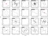 |
Fig. 1 uv coverage for each source. The observations from MIDI are shown in black, while the Keck data from Monnier et al. (2009) are shown in red (only available for select sources). |
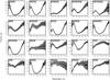 |
Fig. 2 Total N-band spectra of the sources measured with MIDI. |
3.1. Long-baseline interferometry with VLTI
Observations with the MIDI instrument at the VLTI facility of the European Southern Observatory (ESO) on Cerro Paranal were performed in the period 2004–2013, using both the 8.2 m Unit Telescopes (UTs) and the 1.8 m Auxiliary Telescopes (ATs). MIDI, operating at the VLTI continuously since 2003, is a two-telescope interferometric instrument, which is capable of measuring both total and correlated (interferometrically combined) flux, spectrally dispersed over the N band (~8–13 μm).
The nominal observation procedure with MIDI has already been described by Leinert et al. (2004), and we refer to that publication for a more detailed discussion, but provide a brief review of the procedure here. All data presented in this work used the prism as the dispersive element (λ/Δλ ≈ 35), and were carried out in the HIGHSENS mode, meaning the correlated flux and photometric measurements are made separately (as opposed to the SCIPHOT mode, where a beam splitter is used to simultaneously measure the interferometrically-combined and individual beams from each telescope). For the photometric measurements, light is passed, in sequence, from each of the two telescopes used in the interferometric measurement through the VLTI optical train to the MIDI instrument, where it is spectrally dispersed and recorded on the detector. Each interferometric and photometric measurement was preceded and/or followed by a calibration measurement of a bright single star of known brightness and diameter. Finally, we note that MIDI can also function as a simple N-band imager, with acquisition images periodically taken to check the beam position on the chip. On the UTs, these images have a pixel scale of 0084, with a field of view of ~ 4″, and can be AO-corrected in the presence of a suitable optical guide star3.
We summarize the interferometric observations of the 24 objects in our sample in Table A.1, where we show the time the fringe track was started, the telescopes/stations used, as well as the projected baseline and position angle. For four of the targets, despite good weather conditions and no apparent technical problems, we did not detect fringes; these non-detections are summarized at the end of Table A.1 and discussed in Sect. 4.4. The uv coverage for the 20 remaining targets is shown in Fig. 1, where black points indicate the MIDI measurements. Besides the observations conducted within the framework of the present survey, we also include the following data previously published by other investigators: one uv point for AFGL 2136 (de Wit et al. 2011), and 6 points for R CrA (Correia et al. 2008). Finally, we note that observations of select sources, obtained within the context of the survey presented here, have already been published by Linz et al. (2009), Follert et al. (2010), Grellmann et al. (2011), Boley et al. (2012).
We reduced all the raw MIDI data (including data published previously) using version 2.0Beta1 (8 Nov. 2011) of the MIA+EWS package (Jaffe 2004). This new version of MIA+EWS includes significant improvements for sources with low correlated flux. In particular, we make use of the faintpipe procedures to create masks from the interference fringe pattern of all the calibrators. For each night and baseline configuration, we create a median mask from the individual calibrator masks, which we use for extracting the correlated flux and total spectra from the science measurements. Possible decreases in flux due to slit loss were not taken into account, as the observed sources are generally much smaller than the MIDI slit width (229 and 052 for the ATs and UTs, respectively).
Calibrated correlated fluxes (in Jy) were computed from the measured instrumental values using all the calibrator measurements on the same baseline configuration in a given night. For each calibrator of known diameter, taken from the van Boekel database of mid-infrared interferometric calibrators (van Boekel 2004), we derive a wavelength-dependent calibration function relating the measured counts/s of correlated flux on the detector to Jy, and take the mean over all calibrators to calibrate the science measurements. For the estimated uncertainty on the calibrated correlated flux, we include both the statistical error derived by MIA+EWS (based on the variation of the correlated flux over the duration of the fringe track) and the variation of the individual transfer functions derived from the calibrator measurements.
For each target, we created a median spectrum of the total N-band flux from the individual photometric measurements with MIDI (again, using all the calibrators on the same baseline configuration in a given night), which we show in Fig. 2. For sources which were measured with both the UTs and ATs, we used only the spectra observed with the UTs. The uncertainty on the total (median) spectra, shown as error bars in Fig. 2, is taken as the standard deviation over the ensemble used in the median.
3.2. Aperture-masking interferometry with Keck-1
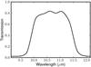 |
Fig. 3 Transmission curve of the Keck 10.6 μm filter. |
For five of the sources in our sample, we also make use of previously-published aperture-masking interferometric observations with the Keck-1 telescope as part of the segment-tilting experiment by Monnier et al. (2009). In contrast to the MIDI observations, these visibility measurements are not spectrally resolved, but rather were taken with a 10.6 μm filter (transmission curve shown in Fig. 3) which covers most of the N-band. The uv coverage provided is uniform, with projected baselines of 0.5−9 m. We show the location of these measurements in uv space as red points in Fig. 1.
Parameters of one-dimensional geometric fits to 10.6 μm visibilities.
4. Results
4.1. Geometric fits to wavelength-averaged visibilities
The MIDI instrument provides spectrally-dispersed interferometric visibilities over the entire N-band, at projected baselines which range from about 5 to 130 m for the observations presented here. However, in order to simplify both the analysis and the combination of the VLTI and Keck observations (available for five of the 20 sources presented here), we examine the complete data set at a single wavelength of 10.6 μm, which corresponds to the center of the filter used for the Keck observations (Fig. 3). In order to directly compare the VLTI and Keck data, we define the mean visibility in the filter as the mean of the correlated flux divided by the mean of the total flux, where each mean is weighted by the filter transmission curve. The uncertainty on the correlated/total flux is taken as the average of the uncertainty over the filter, weighted by the correlated/total flux and the filter transmission.
Extensive uv coverage remains difficult to achieve with long-baseline mid-infrared interferometric observations. In Fig. 1, it can be seen that the coverage ranges anywhere from a single uv point (e.g. M17 UC1) up to several dozen (e.g. IRAS 13481-6124). For some objects, radial coverage is quite good, while measurements at multiple position angles are lacking (e.g. S255 IRS3). For other objects (e.g. M8E-IR), position angles are well sampled, but radial coverage is deficient.
To deal with this variety of uv coverage, for each target we fit up to a maximum of four geometric models to the visibility levels at 10.6 μm, depending on the distribution of observations in uv space. In order of increasing complexity, these models are: a one-dimensional Gaussian (denoted “1D”, parameterized only by the FWHM of the Gaussian); a one-dimensional Gaussian plus an overresolved component (“1DOR”, parameterized by the visibility V(0) of the overresolved component and the FWHM); a two-dimensional Gaussian plus an overresolved component (“2DOR”, parameterized by V(0), the FWHM along the major axis, position angle φ and inclination angle θ); and a two-dimensional Gaussian plus a one-dimensional Gaussian (“2D1D”, parameterized by the ratio of the integrated fluxes F2D/F1D of the two components, their respective sizes FWHM2D and FWHM1D, as well as φ and θ). For the two-dimensional models, we constrain the two components to be centered, meaning all the models are point symmetric. This is consistent with the low differential phases (≲10°) measured for most targets/baselines; exceptions to this (Mon R2 IRS3 A and Orion BN) are discussed in Sect. 5.4.
For the purposes of the present study, we chose not to consider potential contributions from unresolved point sources, as at mid-infrared wavelengths the level of photospheric emission in these objects is expected to be negligible compared to that of the circumstellar material. Additionally, we note that the work of Monnier et al. (2009), which examined a larger sample of intermediate- and high-mass YSOs by means of mid-infrared aperture-masking interferometry, did not find evidence for point-source contributions in these objects. Nevertheless, we note that a few objects in our sample (e.g. V921 Sco, VY Mon) still show visibilities ≳10% at baselines longer than 100 m, meaning that the contribution from an unresolved component in some sources may be on the order of 10–20%.
Parameters of two-dimensional geometric fits to 10.6 μm visibilities.
We show the best-fit parameters for each of these models in Tables 2 (one-dimensional models) and 3 (two-dimensional models). The best-fit models are found using a grid search over parameter space, followed by a downhill-simplex χ2-minimization routine. For each fit, we report the value of  , i.e. the goodness-of-fit parameter divided by the number of degrees of freedom of the fit. Blank rows in Tables 2–3 indicate cases where either the number of model parameters exceeds the number of observed uv points, or the fit did not converge (e.g. due to way the observations are distributed in uv space).
The uncertainties on the fitting parameters are derived using a Monte-Carlo approach, where we generate synthetic observations, normally distributed about the mean observed visibility level with a standard deviation equal to the measurement uncertainty, and repeat the optimization process. In Fig. 4, we show the observed 10.6 μm visibility levels as a function of spatial frequency for each source, together with each best-fit model. The image intensity distributions of the best-fit models are shown in Fig. 5 (spatial scale in mas) and Fig. 6 (spatial scale in AU, using the distances from Table 1).
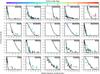 |
Fig. 4 Best-fit geometric models to the 10.6 μm visibilities. The observations are shown as crosses with error bars; the color corresponds to the position angle of the measurement, shown in the color bar at the top of the plot. The 1D model is shown as a solid line, and the 1DOR model is shown as a dotted line. The triangles show the 2DOR model, while the squares show the 2D1D model. For a description of the different models, see Sect. 4.1. |
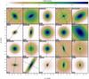 |
Fig. 5 Intensity distributions of the best-fit models described in Sect. 4.1. The model parameters are shown in Tables 2 and 3. Where available, we have indicated outflow and/or disk orientations as dashed and dotted lines, respectively (see Table 1 for disk/outflow directions and references). |
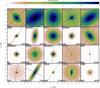 |
Fig. 6 Same as Fig. 5, but the images have been scaled to linear distances in AU using the distances from Table 1. |
4.2. Characterization of the spectrally-dispersed correlated flux levels
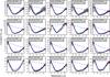 |
Fig. 7 Measured correlated flux spectra (solid black line and error bars) for Orion BN, in order of increasing projected baseline. The caption shows the projected baseline and position angle of each observation. The dashed blue line shows a continuum fit to the red points, and the solid blue line shows the best fit to the absorption spectrum (see Sect. 4.3). |
Besides the wavelength-averaged visibility levels, the MIDI measurements can also be considered in terms of their spectral behavior. In this section, rather than focusing on the visibility amplitude (i.e., the ratio of the correlated flux to the total flux), we consider the correlated flux measured in each observation.
We show the correlated flux as a function of wavelength for each point in uv space for one source, Orion BN, in Fig. 7. The remaining objects are presented in Figs. A.1–A.19. In general, we note that sources which show silicate absorption in their total N-band spectra (Fig. 2) also show absorption in the correlated flux. Qualitatively, this is to be expected, as foreground material (which may include an extended envelope, in addition to the diffuse ISM) will indiscriminately absorb emission from all spatial scales. However, departures from this may be observed if the absorption occurs on scales resolved by MIDI. Additionally, the contribution of emission to the total and (spatially-filtered) correlated flux levels can, in general, depend on both the spatial distribution and spectral characteristics of the emitting material.
In order to evaluate the depth of the silicate feature in each individual spectrum, we fit a continuum in the form of a power law, shown as a blue line in Figs. 7 and A.1–A.19, to the maxima of the correlated flux in the ranges 7.5–8.2 μm and 12.4−12.8 μm (shown as red points in the figures). We evaluate the optical depth of the silicate feature as 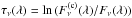 , where Fν is the measured correlated flux, and
  is the continuum fit.
Optical depth of the silicate absorption feature at a wavelength of 10.2 μm.
In Table 4, for the sources which show silicate absorption, we show the derived optical depth at a wavelength of 10.2 μm4. We show both the optical depth τν(10.2 μm) of the feature in the total spectrum, as well as the mean optical depth < τν(10.2 μm) > of the feature in the correlated flux spectra, where we have taken the mean value and standard deviation στν of each target over all the observed baselines and position angles.
4.3. Fitting the correlated flux absorption spectra
A common approach used to model mid-infrared spectra, much simpler than full radiative transfer modeling, is to fit the observed spectrum with a blackbody or power-law spectrum, modified by experimental and/or laboratory dust opacities. For objects which show little or no silicate absorption, this approach has been used to model the mid-infrared emission features seen in T Tauri stars (e.g. Olofsson et al. 2010) and Herbig Ae/Be stars (e.g. Juhász et al. 2010).
Here, we apply a similar approach to the absorption spectra of 13 of the objects in our sample, which have spectra dominated by silicate absorption5. In our model, we let the correlated flux Fν be described by a power-law continuum extincted by foreground material, i.e.  (1)where the constant C and the exponent p, both baseline-dependent, define the continuum. The absorption optical depth τν(λ) is 1) given by the product of the column density and extinction cross-section (defined by the dust composition) of the absorbing material, and 2) defined to be the same for all baselines/position angles. In this context, this “foreground” absorbing material then includes components from both the source envelope, in addition to the diffuse ISM along the line of sight, with the former most likely being the dominant contributor.
For the dust components, we limit ourselves to two sizes each (0.1 and 1.5 μm) of spherical grains of amorphous material, in the form of olivine (Mg2xFe2−2xSiO4) and pyroxene (MgxFe1−xSiO3) glasses. We find that the opacities of pure Mg2SiO4/MgSiO3 grains presented by Jäger et al. (2003) are unable to reproduce the observed absorption spectra, while the inclusion of iron in the silicates leads to satisfactory fits. We therefore adopt x = 0.5 (equal Mg/Fe content) and calculate mass absorption coefficients for each grain type and size, shown in Fig. 8. These absorption coefficients were calculated using Mie theory and the optical properties of the grains from Dorschner et al. (1995). We note, however, that Min et al. (2005) have shown that pure Mg-rich silicates (x = 1.0) yield 10 μm silicate features of nearly identical shape to the iron-rich silicates that we use, if the mass absorption coefficients are calculated for a statistical distribution of grain sizes and shapes6. Hence, our choice of silicate composition should be seen as a practical way of matching the observed silicate features, although it does not provide evidence for the presence of iron in the observed silicates.
This simplified model makes two important assumptions about the correlated flux spectra which may not hold in all cases. Namely, that the underlying emission is well-described by a power law, and that the foreground absorbing screen, which implicitly includes contributions from both an envelope and the diffuse ISM, is independent of spatial scale. Deviations from a power law for the emission can occur not only in the form of spectral features in the emitting material, but can also arise from signatures of the spatial structure in the correlated flux (e.g. from a binary signal or zero crossings in the visibility amplitude). That the foreground absorbing screen is independent of spatial scale means that this absorbing material is essentially uniform on the spatial scales probed by the observations. This may not be true, for example, if significant absorption is occurring at scales already resolved by MIDI. These two assumptions are difficult to verify a priori, but for now we merely take them as postulates, and discuss their validity for individual sources in Sect. 5.4.
In total, for a source with n correlated flux spectra (i.e., n points in uv space, where each point represents a spectrum with ~ 100 wavelength channels), there are 2n + 4 free parameters in this model (2n parameters for the power-law continua, and 4 parameters describing the column densities of each dust type/size). We use a downhill-simplex χ2-minimization routine to optimize all 2n + 4 parameters simultaneously. For an initial solution, we fit a continuum as described in Sect. 4.2, take an equal mix of the four grain types/sizes, and let the total optical depth at 10.2 μm be equal to unity. We derive uncertainties on the fit parameters using a Monte-Carlo approach, where we generate synthetic correlated flux values, normally spread about the observed values, with a standard deviation equal to the noise (i.e., random) error on the measurement as derived by the MIA+EWS package7 and repeat the fit procedure 100 times; the optimum model parameters and their uncertainties are given by the mean and standard deviation, respectively, of the parameters in this ensemble. We show the best-fit models using this procedure as a solid blue line in Figs. 7 and A.1–A.19, and list the total column densities of the absorbing material and the relative mass fraction of each dust component in Table 5.
4.4. Non-detections
For four of the 24 targets which we attempted to observe with MIDI, we were unable to find interferometric fringes despite good technical and weather conditions. Thus, for the observations listed at the end of Table A.1, these sources were completely overresolved by the interferometer. In this section, we discuss each of these non-detections in turn.
4.4.1. GGD 27-ILL
The star-forming region GGD 27 received early attention when Gyulbudaghian et al. (1978) revealed the presence of two strong Herbig-Haro objects in the vicinity. These were later cataloged as HH 80/81, which is the name under which this region is known in the radio astronomy community. The central cm radio source is associated with the infrared source IRAS 18162-2048 (Rodríguez & Reipurth 1989), and drives a thermal ionized jet with bipolar components spanning a total extent of 5.3 pc (Marti et al. 1993). Recent (sub-)mm interferometry indicates that this jet-driving source is associated with a rotating molecular disk (e.g., Fernández-López et al. 2011; Carrasco-González et al. 2012). The central source is not directly visible at wavelengths <3 μm, but its location was inferred by means of near-infrared polarimetry of the surrounding reflection nebula by Tamura et al. (1991). Subsequently referred to as GGD 27-ILL, the central source was later detected at 10 μm (Stecklum et al. 1997), 4.7 μm (Aspin et al. 1994), and even 3.8 μm (Linz et al. 2003).
We attempted to observe GGD 27-ILL in June 2004. A fringe search was performed on the UT2-UT3 baseline, with a projected length of 44 m and a position angle of 22°, which is well-aligned with the ionized jet. No fringes could be found, and no further attempts were possible on the following days due to technical problems during this MIDI commissioning run. However, during this period MIDI could be used as a simple mid-infrared imager. An acquisition image with a total exposure time of 125 s using the narrow-band [Ne ii] filter, shown in Fig. 9, reveals that the source appears slightly extended at mid-infrared wavelengths already with an 8 m-class telescope. Another attempt to observe this source on June 30, 2010 was foiled by poor atmospheric conditions during that night, when even a valid acquisition8 of the target (~5 Jy at 11.7 μm) could not be achieved with the UTs.
4.4.2. IRAS 16164-5046
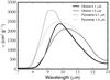 |
Fig. 8 Mass absorption coefficients for amorphous MgFeSiO4 (solid lines) and amorphous Mg0.5Fe0.5SiO3 (dotted lines). Black lines are for a grain radius of 0.1 μm, and the gray lines are for a grain radius of 1.5 μm. |
This source was identified as a YSO by Braz & Epchtein (1987) based on infrared photometry and SED arguments. It is associated with an UCH ii region (e.g., Urquhart et al. 2007). Bik et al. (2006) revealed the presence of CO overtone emission at 2.3 μm in a K-band spectroscopic survey, where this source is referred to as 16164nr36369 in their nomenclature. The same data were used by Bik & Thi (2004) for more detailed modeling of the CO line profiles. They propose that the CO overtone emission from this source arises in a circumstellar disk with an inclination of ~ 30°. Combined with the SED and radio data listed by Bik et al. (2006), and adopting a distance of 3.8–4.0 kpc (Urquhart et al. 2012; Moisés et al. 2011), this indicates the presence of a circumstellar disk around a mid- to late O-star. Wheelwright et al. (2010) refined the 2.3 μm CO line spectroscopy for this source (G332.8256-00.5498 in their nomenclature) by applying spectroastrometric techniques. While no significant spectroastrometric signal could be revealed, the disk interpretation for the CO emission was re-enforced, and an updated disk inclination of 42.3 deg was derived.
We attempted to observe this target with three intermediate AT baselines between 30 and 65 m. In all cases, the fringe search was not successful. In combination with the moderate inclination of 42° for the potential circumstellar disk, this may indicate the existence of a substantial envelope around this object, and hence the related mid-infrared emission might be overresolved by MIDI. In addition, the UCH ii region associated with this source may also give rise to extended mid-infrared emission.
4.4.3. IRAS 17136-3617
Derived column densities and relative contributions (by mass) of absorbing material.
We attempted to observe IRAS 17136-3617 (aka GM 24) two times with MIDI, using projected baselines of 25 and 46 m. However, despite successful acquisition and good weather conditions, no fringes were found, indicating the source is completely overresolved at these baselines. We show a spectrum of the total flux, measured with the 8.2 m UT telescopes, in the left panel of Fig. 10. We note the distinct absence of any silicate absorption feature, despite the apparently large visual extinction of the near-infrared source IRS 3A (AV ≳ 50 mag; Tapia et al. 2009), with which the mid-infrared source is probably associated. This source also represents the only detection of the [Ne ii] nebular emission line at 12.8 μm in our sample.
4.4.4. Orion SC3
Thermal infrared imaging of the Orion Trapezium region, including the famous Ney-Allen nebula, revealed the presence of arc-shaped structures pointing towards the most luminous (multiple) star in the Trapezium, θ1 Ori C (Hayward et al. 1994). Among these newly-found structures was the peculiar object SC3, which appears circularly symmetric at 8.8 and 11.7 μm, despite a very small projected distance (18) from the O6.5 star θ1 Ori C. Robberto et al. (2002) hypothesize SC3 to be a face-on circumstellar disk in the background of θ1 Ori C, which by chance is projected close to the O star.
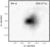 |
Fig. 9 Acquisition image of GGD 27-ILL obtained with UT3 on 2004-06-03 using the [Ne ii] narrow-band filter (center 12.80 μm, width 0.21 μm). North is up, east is left. |
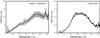 |
Fig. 10 Total spectrum of IRAS 17136-3617 (left) and Orion SC3 (right) measured with the 8.2 m UT telescopes on 2006-05-18 and 2005-02-26, respectively. The error bars represent the uncertainty in the absolute flux calibration. |
We performed one fringe search utilizing the shortest UT baseline UT2-UT3 in February 2005. We did the initial centering on the mid-infrared peak; the neighboring O star, which also shows weak mid-infrared emission (cf. Robberto et al. 2005), is outside the field of view for these MIDI UT observations. No fringes were detected. Hence, given the low total flux of SC3 of <2 Jy, a source with a large fraction of extended emission will give rise to very low correlated flux levels, which may not be detectable by MIDI. Mid-infrared imaging with T-ReCS at Gemini South from the same year (Smith et al. 2005) gives some credence to this suggestion: their single-dish resolution is sufficient to spatially resolve SC3 into a compact peak surrounded by a more extended halo with a size of  . The spectrum of the total flux, shown in the right panel of Fig. 10, shows a clear silicate emission feature, which supports the interpretation of a circumstellar disk with low inclination. We note the absence of the [Ne ii] 12.8 μm line, which we find consistent with the idea that SC3 is not directly subjected to the intense radiation from the Trapezium O star θ1 OriC.
5. Analysis and discussion
5.1. N-band geometry
The results of the geometric modeling described in Sect. 4.1 show a range of linear sizes and inclinations. In general, the mid-infrared intensity distributions of the sources are not circularly symmetric: when our uv coverage is sufficient to fit a two-dimensional model, we find inclinations ranging from 30° to 80° (corresponding to axial ratios of about 1.15 to 6), indicating the presence of non-spherical structures on scales of tens of milliarcseconds.
For 12 of the targets observed in our sample, independent information about disks and/or outflows is available in the literature, which can provide insights into the physical nature of the asymmetries present in the MIDI data. In Figs. 5 and 6, we show, where available, orientations collected from the literature (see Table 1 for values and references) for circumstellar disks (dotted lines) and/or outflows (dashed lines).
In general, we see a tendency for the compact, mid-infrared emission to trace disk structures, albeit with exceptions. As extreme cases, the compact, mid-infrared emission of AFGL 2136 is both elongated along the direction of the circumstellar disk and perpendicular to the outflow, while the situation in the case of M8E-IR appears to be reversed: the MIDI visibilities seem to trace an outflow component (no disk detection for this object has been reported in the literature). For six sources with known disks and/or outflow components, and where we fit a two-dimensional geometric model (IRAS 13481-6124, MWC 300, R CrA, R Mon, S255 IRS3, and V921 Sco), the structures resolved by MIDI are roughly parallel to the disk/perpendicular to the outflow. In the case of Mon R2 IRS3 A, the mid-infrared emission is roughly perpendicular to the polarization disk reported by Yao et al. (1997). This and other sources are discussed in more detail in Sect. 5.4.
Finally, we note that the geometric analysis of the wavelength-averaged visibilities presented here represents only a first attempt at understanding the physical structures responsible for emission in these sources. In particular, analyses of the wavelength dependence of the visibilities have the potential to unlock a wealth of additional information about these objects, and we encourage such endeavors.
5.2. Mid-infrared size vs. luminosity
At near-infrared wavelengths, using a model consisting of a thin ring representing the inner radius of a circumstellar disk, Monnier & Millan-Gabet (2002) showed a tight correlation between luminosity and ring radius for YSOs with luminosities in the range ~ 100–105L⊙. This correlation arises both because the dust sublimation radius varies with  (e.g. Monnier & Millan-Gabet 2002), and because the near-infrared emission from grains near the dust evaporation temperature (~1500 K) is confined to a small region of the disk. This relation seems to break down at higher luminosities (L ≳ 104L⊙), which may indicate the presence of optically-thick circumstellar gas interior to the dust evaporation radius (Monnier et al. 2005).
The relation between size and luminosity has been examined at mid-infrared wavelengths, as well. Using the FWHM of a Gaussian fit to the mid-infrared visibilities, Monnier et al. (2009) and Grellmann et al. (2011) found that although the mid-infrared size of YSOs is correlated with luminosity, there is considerably more scatter in the relation than is seen at near-infrared wavelengths. Indeed, this is to be expected; as noted in both these works, at mid-infrared wavelengths the notion of “size” becomes more complex than a simple ring radius: the mid-infrared intensity distribution is complicated by a combination of geometrical effects (e.g. flaring, shadowing), temperature/wavelength effects (the extent of the near-infrared emission is limited by the Wien cut-off at the dust sublimation temperature) and the fact that the mid-infrared radiation is expected to arise from a variety of structures (e.g. disk wall, disk surface, envelope).
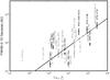 |
Fig. 11 Linear size vs. luminosity. The black crosses show the sizes derived in this work from the one-dimensional Gaussian models for selected sources (see Sect. 5.2), while the gray crosses show the results compiled by Grellmann et al. (2011). The solid line shows a fit to the black points for |
For sources for which the luminosity is known, we show the FWHM size we derive from the one-dimensional Gaussian geometric model vs. luminosity as black crosses in Fig. 11, together with the sizes and luminosities compiled by Grellmann et al. (2011) as gray crosses. In our own sample, in order to restrict ourselves to sources where we do not completely overresolve the extended structure with the interferometer, we limit the selection to those sources for which we measure V ≳ 0.5 at the shortest baselines. Besides the uncertainty on the derived angular size, in the derivation of the linear size we also account for the uncertainty in the distance to each source. If no value for the uncertainty in distance is available in Table 1, we adopt a value of 25%, which is appropriate for kinematic and photometric distances. As both Monnier et al. (2009) and Grellmann et al. (2011) found, we see considerable scatter in the mid-infrared size vs. luminosity relation. A scaling relation of  , shown as a black line in Fig. 11, is consistent with the mid-infrared sizes, but is by no means as well-defined as at near-infrared wavelengths.
5.3. Absorption spectra and dust composition
As Table 4 shows, the optical depth of the silicate absorption feature is sometimes substantially lower in the total spectrum than it is in the correlated flux spectra. This is probably due to the fact that the total spectrum contains contributions of emission from all scales, while the spatial filtering of the interferometer limits this contribution to a single scale in each correlated flux spectrum. In this context, the true shape of the absorption feature is best represented in the short-baseline interferometric measurements, where contributions from hot emitting material (which is presumably more dominant at smaller spatial scales) are minimized.
In general, we find that the power-law emission/foreground absorption model described in Sect. 4.3 for the 13 sources in Table 5 adequately reproduces the observed correlated flux spectra in almost all cases (the fits for the sources from Table 5 are shown as blue lines in Figs. 7 and A.1–A.19). As the column density and composition of the absorbing material is constrained to be the same for all baselines, this means that the absorption (due to silicates) is both uniform over the spatial scales probed by MIDI, and physically detached from those scales. Furthermore, the underlying emission also seems to be well-approximated by a power law.
There are, however, some cases where this simple model is unable to reproduce the observed correlated flux levels. For example, for AFGL 4176 (Fig. A.2) the fits at short baselines are quite good, but become progressively worse at long baselines. At the longest spatial scales, the imprint of the spatial structure on the correlated flux levels becomes apparent (Boley et al. 2012), meaning that the assumption of the underlying emission having a power-law spectrum is incorrect. Such spatial effects may also be present in G305.20+0.21 (Fig. A.3) and Mon R2 IRS3 A (Fig. A.10).
Besides effects from the source geometry, the true emission spectrum behind the foreground absorption screen may, in the general case, contain spectral features (from, for example, silicates, crystalline grain species, etc.). Such features may become more prominent at longer baselines due to potential emission arising from a circumstellar disk (e.g van Boekel et al. 2004). However, accounting for emission features in the spectra of deeply-embedded sources is a complicated process, and beyond the scope of the present work.
As shown in Table 5, for most sources the majority of the absorbing material can be attributed to amorphous (glass) olivine. AFGL 2136 stands alone in being clearly dominated by amorphous pyroxene, while AFGL 4176 and NGC 2264 IRS1 have roughly equal contributions (by mass) of amorphous pyroxene and olivine dust. Three sources (AFGL 2136, AFGL 4176 and M8E-IR) show a significant population of large grains (1.5 μm), but for the other ten sources fit the amount of mass contained in large grains is limited to a few percent. In general, however, we find that the grain size distribution, and to some extent the grain composition, is highly variable throughout our sample. Although this is expected, given the qualitatively different shapes of the silicate absorption feature in both the total and correlated flux spectra, it should be taken as a reminder when modeling these and other similar objects that the dust composition may differ significantly from that of the diffuse interstellar medium.
Finally, we note that while the exact proportions derived for the grain species and listed in Table 5 are dependent on the opacity templates used (see Sect. 4.3), the general trends derived from fitting the dust features of mid-infrared spectra (size distribution, pyroxene/olivine ratio) have been shown not to depend strongly on the specifics of the grains (e.g. Juhász et al. 2009). In this sense, regardless of the specifics of the iron content or grain structure (shape, porosity, etc.) of the amorphous silicates used, larger grains tend to give a wider 10 μm feature relative to smaller grains, and the center of this feature tends to be at shorter wavelengths for grains with a pyroxene stoichiometry than for grains with an olivine stoichiometry. Thus, the general conclusions about the size distributions and olivine/pyroxene ratios derived in Sect. 4.3 can be considered robust. For further discussion of this topic, we direct the interested reader to the works by Bouwman et al. (2008) and Juhász et al. (2010), and references therein.
5.4. Notes on selected sources
5.4.1. AFGL 2136
AFGL 2136 IRS1 is from the classic list of BN-type objects (Henning et al. 1984). It is the illuminating infrared source of the so-called Juggler reflection nebula (Kastner et al. 1992). Menten & van der Tak (2004) found faint centimeter emission (their component RS4) closely associated with this target. The nature of this emission, which is optically thick up to frequencies of ~43 GHz, is not clarified yet, although an ionized jet is the most probable explanation. As mentioned in Sect. 5.1, the sizes derived from the MIDI visibilities for AFGL 2136 show significant elongation parallel to the major axis of a circumstellar disk, which was revealed in near-infrared polarimetric images by Minchin et al. (1991), and perpendicular to the molecular outflow found by Kastner et al. (1994). The FWHM size of the two-dimensional Gaussian in our geometric model is 44 mas (88 AU at 2 kpc), and the correlated flux levels are well reproduced by the foreground-absorption model described in Sect. 4.3 (see Fig. A.1).
5.4.2. AFGL 4176
AFGL 4176 is a southern high-luminosity MYSO (Henning et al. 1984; Persi et al. 1986). The position angle and elongation derived from the 2D1D model here are consistent with the more complicated temperature-gradient disk model presented by Boley et al. (2012). The correlated flux (Fig. A.2) is reproduced well by our absorption model at shorter baselines, with the fits becoming progressively worse towards longer baselines, which we find consistent with the expectation that emission at these angular scales is dominated by hot dust (Boley et al. 2012).
5.4.3. G305.20+0.21
The surveys presented by Walsh et al. (1999, 2001) established the presence of a bright compact infrared source within the star-forming complex G305. There is an H ii region some 10′′ to the southwest (Walsh et al. 2007), but the infrared source itself is not associated with centimeter free-free emission (Phillips et al. 1998; Walsh et al. 2007). The extrapolated IRAS luminosity is ≳105L⊙ (Walsh et al. 2001), which together with the cm non-detection supports our view that this object is a MYSO in a pre-UCH ii-region stage. Further interest is triggered by the presence of a group of aligned class-II methanol masers coincident with this infrared object (component G305.202+0.207 in the work by Phillips et al. 1998). Soon after the finding of a number of such sources (including G305), it was speculated that such aligned masers might trace edge-on circumstellar disks (Norris et al. 1998). However, there is also evidence that methanol maser distributions may instead trace outflows (e.g. De Buizer 2003; De Buizer et al. 2012).
The geometric fits for this object indicate a large (200 AU at 4.8 kpc) structure, elongated along a position angle of ~ 34°. This is roughly consistent with the orientation of the linear maser distribution of ~57° found by Norris et al. (1998); however, as noted above, it is not clear that the maser orientation can be readily attributed to a disk or an outflow. The correlated flux levels (Fig. A.3) show features which cannot be reproduced by our absorption model.
5.4.4. IRAS 13481-6124
Though it was identified as a MYSO in the 1980 s (Persson & Campbell 1987), and was found to feature an ionized wind (Beck et al. 1991), there were not many more observational studies available for this southern object until recently. The discoveries of both a disk and a jet/outflow system, however, have been recently reported around this MYSO (Kraus et al. 2010; Stecklum et al. 2010).
The uv coverage of the MIDI observations of this source is extensive, and the orientation derived from the 2D1D geometric model (position angle ~ 112°) is consistent with the near-infrared disk (Kraus et al. 2010). The correlated flux levels (Fig. A.4) are well reproduced by our absorption model at all baselines.
5.4.5. IRAS 17216-3801
After its initial identification as a MYSO by Persson & Campbell (1987), this interesting source has been somewhat neglected. This may have been caused by its location on the southern sky, and more than 1° away from the Galactic plane. It is very bright in the K band, which enabled early speckle observations by Leinert et al. (1997, 2001). However, these revealed just a faint (scattering) halo, but no more complex, spatially-resolved structures, and no binarity. The object bears some resemblance to IRAS 13481-6124 in terms of infrared appearance and luminosity, but the presence of outflow or jet activity has not yet been investigated.
The 2DOR geometric model shows that the two-dimensional component needs to be quite large in linear scale (FWHM ~ 260 AU at 3.1 kpc) in order to fit the data. The correlated flux spectra shown in Fig. A.5, as well as the total N-band spectrum, have an unusual triangular appearance which is only partially reproduced by our simple absorption model.
5.4.6. M8E-IR
The study by Simon et al. (1984) was the first work to disentangle the M8 East region into an UCH ii region with no near-infrared counterpart10 and a strong infrared source, subsequently called M8E-IR, which is around 7′′ away. Simon et al. (1984) emphasized the similarities between M8E-IR and the BN object in Orion. M8E-IR was later confirmed not to be associated with free-free emission from ionized gas at wavelengths of 2 and 6 cm (cf. Molinari et al. 1998,and their source region Mol 37). Simon et al. (1985) speculated on the existence of a small circumstellar disk around M8E-IR based on thermal infrared lunar occultation data. Their indications for a small elongated structure came mainly from their 3.8 μm data, while their 10 μm data are in agreement with a more symmetric intensity distribution.
Our geometric fits of this object show that the compact mid-infrared emission is elongated along the CO outflow reported by Mitchell et al. (1991). This is consistent with the work of Linz et al. (2009), who concluded that the role of a circumstellar disk in this system is probably negligible.
5.4.7. M17 SW IRS1
This object is in the list of BN-type objects by Henning et al. (1984). It is also known as the Kleinmann-Wright (KW) object (Kleinmann & Wright 1973), and is situated in the dusty south-western part of the M17 star-forming complex. Porter et al. (1998) analyzed the H- and K-band spectra of this object, and concluded that they resemble the spectrum coming from a concealed Herbig Be star. Chini et al. (2004) revealed multiplicity within a few thousand AU in the near-infrared. However, the actual KW object is the dominating YSO in that core region, and is estimated to have a luminosity equivalent to that of an early B-type star. Follert et al. (2010) originally published the MIDI data included here, and used them to select appropriate models from the Robitaille et al. (2007) model grid of YSOs. Our geometrical analysis agrees with their assessment that a strongly-inclined configuration (θ ≳ 60°) is necessary to explain the observations.
5.4.8. M17 UC1
This object is a deeply-embedded young massive star in the M17 complex. It is known to be associated with a hyper-compact H ii region (Felli et al. 1980, 1984) with an electron density of greater than 105 cm-3. Additionally, broad (≳35 km s-1) radio recombination lines have been found (Johnson et al. 1998). One of the interpretations for such line widths, which are in excess of the usual Doppler broadening, is the infall of material onto, and/or the rotation of, an accretion disk (e.g. Sewilo et al. 2004). In the infrared, Chini et al. (2000) found that UC1 is weak at 1–2.2 μm wavelengths. However, there is another infrared source ~ 9000 AU away (IRS 5S), which is a stronger source in the near-infrared (but similarly bright in the N-band) which might form a bound high-mass system together with UC1.
This object was not in our original target list, but was observed as a backup target during a different MIDI program on our request. Therefore, we have only a single visibility measurement. Hence, we can just derive a one-dimensional Gaussian size. Nevertheless, these data show that it is at least possible to obtain fringes for hyper-compact H ii regions. The mid-infrared emission is not overresolved as a whole, as might be the tendency for more-evolved ultra-compact H ii regions (see our example of IRAS 17136-3617 in Sect. 4.4).
5.4.9. Mon R2 IRS2
Mon R2 is a massive star forming region, with an UCH ii region lying just off the center of a molecular core. There are several well-known compact infrared sources around this region, among them Mon R2 IRS2. IRS2 is situated in the geometrical center of a ring-like near-infrared structure, and has been shown to be the main source of illumination (Aspin & Walther 1990). Furthermore, a large-scale bipolar CO outflow exists in the region (e.g. Giannakopoulou et al. 1997), but its association with IRS2 is not established (e.g., Jaffe et al. 2003). IRS2 has a strong infrared excess, but is not a source of free-free emission. It is unresolved in K-band speckle observations with UKIRT (Alvarez et al. 2004). The extent of the mid-infrared emission we find is quite compact (≲40 AU at 830 pc), which might be an imprint of the lower luminosity of Mon R2 IRS2.
5.4.10. Mon R2 IRS3 A
The IRS3 region is another activity center within the Mon R2 star-forming complex. Several near-infrared speckle studies have addressed the multiplicity on arcsecond scales (Koresko et al. 1993; Preibisch et al. 2002; Alvarez et al. 2004). The dominating source at 2 μm, as well as 10 μm, is IRS3 A (using the same nomenclature as Preibisch et al. 2002). This source is surrounded by a bipolar near-infrared nebula (position angle ~ 30°), suggesting it to be embedded in a thick disk or torus, with pronounced polar cavities.
The MIDI visibilities are low, and most of the correlated flux spectra are box-like and cannot be reproduced by our absorbing dust models (Sect. 4.3). The fit with the 2D1D model, using the combined MIDI and Keck data, yields a position angle of 41°, i.e. similar to the orientation of the near-infrared bipolar nebula, and consistent with the fit to the Keck data by Monnier et al. (2009). Finally, we note that the MIDI data show differential phases significantly deviating from zero, which is indicative of deviations from point symmetry.
5.4.11. Mon R2 IRS3 B
A second YSO is visible in the mid-infrared in the vicinity of Mon R2 IRS3 A, located 083 to the north-east (cf. Monnier et al. 2009), termed IRS3 B by Preibisch et al. (2002). A high-velocity outflow was found by Giannakopoulou et al. (1997) roughly perpendicular to the dominating molecular outflow in Mon R2 IRS3, which itself has a position angle of ~135°. Preibisch et al. (2002) speculate that IRS3 B might be the driving source for this high-velocity flow, based on the near-infrared appearance of shocked H2 blobs along a position angle of 50°, which seem to emanate from this source. This suggests a collimating circumstellar structure around IRS3 B, oriented roughly perpendicular to the shock features at 50°.
With MIDI, IRS3 B shows higher visibility levels than IRS3 A, but is clearly weaker regarding the total N-band flux. Therefore, MIDI observations were only possible using the UTs. The two measurements, with nearly perpendicular baseline angles (but similar projected baseline lengths) show the highest optical depth in the silicate absorption feature of the correlated fluxes among all of our targets (see Table 4 and Fig. A.11). The two correlated flux spectra show some differences in shape, but the general flux levels are not drastically different. Given that the two MIDI baseline angles are roughly parallel and perpendicular to the potential disk, this suggests that this disk is not seen edge-on, but instead at a moderate inclination. Contrary to IRS3 A, the absorption of the correlated flux from IRS3 B is reproduced well by our absorption model.
5.4.12. Orion BN
This very strong near- and mid-infrared source was recognized by Becklin & Neugebauer (1967) as a distinct brightness peak within the Orion KL region. Although it quickly achieved the status of a prototype object for a sample of high-mass protostars (e.g., Henning et al. 1984), many details about the nature of Orion BN are still unclear. The peculiar proper motion of BN is well-established (Plambeck et al. 1995), however, the actual origin of this object is still debated. It might stem from the dissolution of a multiple system in Orion KL itself (e.g. Rodríguez et al. 2005; Gómez et al. 2008), while another group proposes Orion BN to be a runaway source, ejected from the Orion Trapezium (Tan 2004; Chatterjee & Tan 2012). The mid-infrared peak of BN is surrounded by extended emission, with a pronounced extension to the southwest, and the compact emission shows a barely-resolved elongation along the northwest-southeast direction in the Keck 12.5 μm imaging by Shuping et al. (2004). Earlier, the presence of an ultra-dense ionized circumstellar wind was revealed (e.g., Scoville et al. 1983), and recent radio recombination line interferometry revealed a velocity gradient of 10 km s-1 in the northeast-southwest direction (Rodríguez et al. 2009), which might indicate motion in an ionized jet. Finally, near-infrared imaging polarimetry revealed polarization patterns consistent with a circumstellar disk, with an elongation along a direction of 126° (Jiang et al. 2005).
Our MIDI data were collected primarily with the ATs, and show the presence of a source which is clearly resolved. The derived angular sizes of the two-dimensional component in arcseconds translates into a relatively small linear size (~10–20 AU). We see clear indications for deviations from spherical symmetry, and the 2D1D geometric model can only fit some of the data points reasonably well. The position angle of the two-dimensional component is around 14°, i.e. roughly consistent with the axis of the disk of 36° proposed by Jiang et al. (2005). However, the quality of the 2D1D model fit is rather poor ( ) and this value may not be well determined. In particular, the data points with position angles of around 70° pose larger problems for the 2D1D model, indicating the presence of more complex structures than can be reproduced with this model. Finally, we note that BN shows significant differential phase signals in the MIDI data (cf. Linz et al. 2008), indicating deviations from point symmetry.
6. Summary and conclusions
In this work, we presented the results of a nine-year program to observe massive young stellar objects with the two-telescope mid-infrared interferometric instrument MIDI on the Very Large Telescope Interferometer of the European Southern Observatory on Cerro Paranal, Chile. We measured spectrally-resolved, long-baseline interferometric visibilities in the 8–13 μm wavelength range for 20 massive YSOs, with projected baselines ranging from 5 to 130 m. Where available, we combined these data with previously-published measurements of the sources in our sample, both from MIDI, and the Keck segment tilting experiment of Monnier et al. (2009).
Using simple geometric models of the visibilities at a wavelength of 10.6 μm, we derived emission scales and showed significant asymmetries in the majority of the objects. Although there is a general trend of increasing mid-infrared size with luminosity, we confirm a much looser correlation than that reported for YSOs at near-infrared wavelengths, as has been found also by Monnier et al. (2009) and Grellmann et al. (2011). A comparison with literature information about disks and/or outflows shows that, in general, neither one of these components is solely responsible for the compact N-band emission. Consequently, caution should be used when attributing mid-infrared emission to a particular physical structure for objects which may have both an outflow and a disk. For some of the objects in our sample, the long-baseline MIDI measurements represent the first detection of any asymmetries; these results can thus be used in planning future observations to directly detect disk and/or outflow components in these sources.
For 13 sources which show a deep silicate absorption feature, we fit a simple model to the correlated flux, consisting of a smooth (power-law) spectrum, extincted by a foreground screen of material with a column density and dust composition (a mix of large and small grains of magnesium-iron silicates, fit for each source) independent of projected baseline or position angle. In almost all cases, this model adequately reproduces the observed correlated fluxes, implying that the absorbing material is both largely uniform, and detached from the spatial scales probed by MIDI. Furthermore, both the grain size distribution and composition vary throughout the sample.
We make the MIDI observations presented here available in reduced, electronic form via the CDS in OIFITS format (for a description of the OIFITS standard, see the work by Pauls et al. 2005), with the hope that they will prove useful for more detailed studies of these massive YSOs.
Online material
Appendix A: Online material
Observation log.
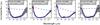 |
Fig. A.1 Measured correlated flux spectra (solid black line and error bars) for AFGL 2136, in order of increasing projected baseline. The caption shows the projected baseline and position angle of each observation. The dashed blue line shows a continuum fit to the red points, and the solid blue line shows the best fit to the absorption spectrum (see Sect. 4.3). |
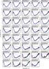 |
Fig. A.2 Measured correlated flux spectra (solid black line and error bars) for AFGL 4176, in order of increasing projected baseline. The caption shows the projected baseline and position angle of each observation. The dashed blue line shows a continuum fit to the red points, and the solid blue line shows the best fit to the absorption spectrum (see Sect. 4.3). |
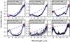 |
Fig. A.3 Measured correlated flux spectra (solid black line and error bars) for G305.20+0.21, in order of increasing projected baseline. The caption shows the projected baseline and position angle of each observation. The dashed blue line shows a continuum fit to the red points, and the solid blue line shows the best fit to the absorption spectrum (see Sect. 4.3). |
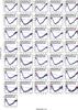 |
Fig. A.4 Measured correlated flux spectra (solid black line and error bars) for IRAS 13481-6124, in order of increasing projected baseline. The caption shows the projected baseline and position angle of each observation. The dashed blue line shows a continuum fit to the red points, and the solid blue line shows the best fit to the absorption spectrum (see Sect. 4.3). |
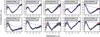 |
Fig. A.5 Measured correlated flux spectra (solid black line and error bars) for IRAS 17216-3801, in order of increasing projected baseline. The caption shows the projected baseline and position angle of each observation. The dashed blue line shows a continuum fit to the red points, and the solid blue line shows the best fit to the absorption spectrum (see Sect. 4.3). |
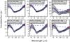 |
Fig. A.6 Measured correlated flux spectra (solid black line and error bars) for M8E-IR, in order of increasing projected baseline. The caption shows the projected baseline and position angle of each observation. The dashed blue line shows a continuum fit to the red points, and the solid blue line shows the best fit to the absorption spectrum (see Sect. 4.3). |
 |
Fig. A.7 Measured correlated flux spectra for M17 SW IRS1, in order of increasing projected baseline. The caption shows the projected baseline and position angle of each observation. |
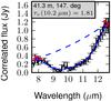 |
Fig. A.8 Measured correlated flux spectra (solid black line and error bars) for M17 UC1, in order of increasing projected baseline. The caption shows the projected baseline and position angle of each observation. The dashed blue line shows a continuum fit to the red points, and the solid blue line shows the best fit to the absorption spectrum (see Sect. 4.3). |
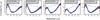 |
Fig. A.9 Measured correlated flux spectra (solid black line and error bars) for Mon R2 IRS2, in order of increasing projected baseline. The caption shows the projected baseline and position angle of each observation. The dashed blue line shows a continuum fit to the red points, and the solid blue line shows the best fit to the absorption spectrum (see Sect. 4.3). |
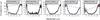 |
Fig. A.10 Measured correlated flux spectra for Mon R2 IRS3 A, in order of increasing projected baseline. The caption shows the projected baseline and position angle of each observation. The dashed blue line shows a continuum fit to the red points. |
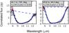 |
Fig. A.11 Measured correlated flux spectra (solid black line and error bars) for Mon R2 IRS3 B, in order of increasing projected baseline. The caption shows the projected baseline and position angle of each observation. The dashed blue line shows a continuum fit to the red points, and the solid blue line shows the best fit to the absorption spectrum (see Sect. 4.3). |
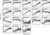 |
Fig. A.12 Measured correlated flux spectra for MWC 300, in order of increasing projected baseline. The caption shows the projected baseline and position angle of each observation. |
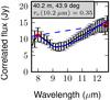 |
Fig. A.13 Measured correlated flux spectra (solid black line and error bars) for NGC 2264 IRS1, in order of increasing projected baseline. The caption shows the projected baseline and position angle of each observation. The dashed blue line shows a continuum fit to the red points, and the solid blue line shows the best fit to the absorption spectrum (see Sect. 4.3). |
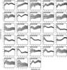 |
Fig. A.14 Measured correlated flux spectra for R CrA, in order of increasing projected baseline. The caption shows the projected baseline and position angle of each observation. |
 |
Fig. A.15 Measured correlated flux spectra (solid black line and error bars) for R Mon, in order of increasing projected baseline. The caption shows the projected baseline and position angle of each observation. The dashed blue line shows a continuum fit to the red points, and the solid blue line shows the best fit to the absorption spectrum (see Sect. 4.3). |
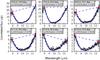 |
Fig. A.16 Measured correlated flux spectra (solid black line and error bars) for S255 IRS3, in order of increasing projected baseline. The caption shows the projected baseline and position angle of each observation. The dashed blue line shows a continuum fit to the red points, and the solid blue line shows the best fit to the absorption spectrum (see Sect. 4.3). |
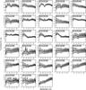 |
Fig. A.17 Measured correlated flux spectra for V921 Sco, in order of increasing projected baseline. The caption shows the projected baseline and position angle of each observation. |
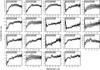 |
Fig. A.18 Measured correlated flux spectra for V1028 Cen, in order of increasing projected baseline. The caption shows the projected baseline and position angle of each observation. |
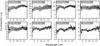 |
Fig. A.19 Measured correlated flux spectra for VY Mon, in order of increasing projected baseline. The caption shows the projected baseline and position angle of each observation. |
Note, the mass of the central object in these systems is generally estimated from the luminosity, as direct measurement of the photospheric spectrum (e.g. Testi et al. 2010) is very difficult.
For example, the distance to the Orion star-forming region, which hosts Orion BN, has been measured very precisely by Menten et al. (2007) using parallax measurements. At the same time, the distance to R Mon has never been measured, yet is generally quoted as being 800 pc, based on distance measurements to a star cluster which is one full degree away from the source on the sky. We regard such determinations as highly uncertain, but defer comments on specific sources to Sect. 5.4.
Although regular acquisition images are not part of the standard ESO observing procedure with MIDI and are not discussed extensively in the present work, some results are discussed briefly in Sect. 4.4.1.
We exclude Mon R2 IRS3 A from this analysis, which has a much wider absorption feature than can be fit by the dust species used here (see Fig. A.10).
Min et al. (2005) use a distribution of hollow spheres (DHS).
Note that the error bars shown in Figs. 7 and A.1–A.19 represent the combination of this random error, plus the uncertainty on the absolute calibration. The absolute flux calibration introduces a factor which varies only slowly with wavelength, and thus is not expected to change the shape of the silicate feature. The random error, which characterizes the wavelength-to-wavelength scatter in the correlated flux of an individual spectrum, is about an order of magnitude smaller than the calibration error.

Infrared emission from the UCH ii region was revealed much later, and only in the mid-infrared at 24.5 μm (Linz et al. 2009; de Wit et al. 2009).
Acknowledgments
We thank J. Monnier for providing the reduced Keck data, J.-U. Pott for observing the object M17 UC1 upon our request, G. Meeus for providing the R CrA data, and J. Bouwman for useful discussions regarding the dust opacities. It is our pleasure to thank the anonymous referee, who carefully reviewed this manuscript and provided helpful critique and suggestions for its improvement.
References
- Alvarez, C., Hoare, M., Glindemann, A., & Richichi, A. 2004, A&A, 427, 505 [NASA ADS] [CrossRef] [EDP Sciences] [Google Scholar]
- Argon, A. L., Reid, M. J., & Menten, K. M. 2000, ApJS, 129, 159 [NASA ADS] [CrossRef] [Google Scholar]
- Aspin, C., & Geballe, T. R. 1992, A&A, 266, 219 [NASA ADS] [Google Scholar]
- Aspin, C., & Walther, D. M. 1990, A&A, 235, 387 [NASA ADS] [Google Scholar]
- Aspin, C., Puxley, P. J., Blanco, P. R., et al. 1994, A&A, 292, L9 [NASA ADS] [Google Scholar]
- Baxter, E. J., Covey, K. R., Muench, A. A., et al. 2009, AJ, 138, 963 [NASA ADS] [CrossRef] [Google Scholar]
- Beck, S. C., Fischer, J., & Smith, H. A. 1991, ApJ, 383, 336 [NASA ADS] [CrossRef] [Google Scholar]
- Becklin, E. E., & Neugebauer, G. 1967, ApJ, 147, 799 [NASA ADS] [CrossRef] [Google Scholar]
- Bik, A. 2004, Ph.D. Thesis, University of Amsterdam [Google Scholar]
- Bik, A., & Thi, W. F. 2004, A&A, 427, L13 [NASA ADS] [CrossRef] [EDP Sciences] [Google Scholar]
- Bik, A., Kaper, L., & Waters, L. B. F. M. 2006, A&A, 455, 561 [NASA ADS] [CrossRef] [EDP Sciences] [Google Scholar]
- Blum, R. D., Barbosa, C. L., Damineli, A., Conti, P. S., & Ridgway, S. 2004, ApJ, 617, 1167 [NASA ADS] [CrossRef] [Google Scholar]
- Boley, P. A., Linz, H., van Boekel, R., et al. 2012, A&A, 547, A88 [NASA ADS] [CrossRef] [EDP Sciences] [Google Scholar]
- Borges Fernandes, M., Kraus, M., Lorenz Martins, S., & de Araújo, F. X. 2007, MNRAS, 377, 1343 [NASA ADS] [CrossRef] [Google Scholar]
- Bouwman, J., Henning, T., Hillenbrand, L. A., et al. 2008, ApJ, 683, 479 [NASA ADS] [CrossRef] [Google Scholar]
- Braz, M. A., & Epchtein, N. 1987, A&A, 176, 245 [NASA ADS] [Google Scholar]
- Brugel, E. W., Mundt, R., & Buehrke, T. 1984, ApJ, 287, L73 [NASA ADS] [CrossRef] [Google Scholar]
- Carrasco-González, C., Galván-Madrid, R., Anglada, G., et al. 2012, ApJ, 752, L29 [NASA ADS] [CrossRef] [Google Scholar]
- Casey, S. C., & Harper, D. A. 1990, ApJ, 362, 663 [NASA ADS] [CrossRef] [Google Scholar]
- Chatterjee, S., & Tan, J. C. 2012, ApJ, 754, 152 [NASA ADS] [CrossRef] [Google Scholar]
- Chini, R., Nielbock, M., & Beck, R. 2000, A&A, 357, L33 [NASA ADS] [Google Scholar]
- Chini, R., Hoffmeister, V. H., Kämpgen, K., et al. 2004, A&A, 427, 849 [NASA ADS] [CrossRef] [EDP Sciences] [Google Scholar]
- Cohen, M., Harvey, P. M., Wilking, B. A., & Schwartz, R. D. 1984, ApJ, 278, 671 [NASA ADS] [CrossRef] [Google Scholar]
- Cohen, R. J., Masheder, M. R. W., & Caswell, J. L. 1995, MNRAS, 274, 808 [NASA ADS] [Google Scholar]
- Correia, S., Köhler, R., Meeus, G., & Zinnecker, H. 2008, in The Power of Optical/IR Interferometry: Recent Scientific Results and 2nd Generation, eds. A. Richichi, F. Delplancke, F. Paresce, & A. Chelli, 175 [Google Scholar]
- De Buizer, J. M. 2003, MNRAS, 341, 277 [NASA ADS] [CrossRef] [Google Scholar]
- De Buizer, J. M., Redman, R. O., Longmore, S. N., Caswell, J., & Feldman, P. A. 2009, A&A, 493, 127 [NASA ADS] [CrossRef] [EDP Sciences] [Google Scholar]
- De Buizer, J. M., Morris, M. R., Becklin, E. E., et al. 2012, ApJ, 749, L23 [NASA ADS] [CrossRef] [Google Scholar]
- de Wit, W. J., Hoare, M. G., Fujiyoshi, T., et al. 2009, A&A, 494, 157 [NASA ADS] [CrossRef] [EDP Sciences] [Google Scholar]
- de Wit, W. J., Hoare, M. G., Oudmaijer, R. D., et al. 2011, A&A, 526, L5 [NASA ADS] [CrossRef] [EDP Sciences] [Google Scholar]
- Dorschner, J., Begemann, B., Henning, T., Jaeger, C., & Mutschke, H. 1995, A&A, 300, 503 [NASA ADS] [Google Scholar]
- Felli, M., Johnston, K. J., & Churchwell, E. 1980, ApJ, 242, L157 [NASA ADS] [CrossRef] [Google Scholar]
- Felli, M., Churchwell, E., & Massi, M. 1984, A&A, 136, 53 [NASA ADS] [Google Scholar]
- Fernández-López, M., Girart, J. M., Curiel, S., et al. 2011, AJ, 142, 97 [CrossRef] [Google Scholar]
- Follert, R., Linz, H., Stecklum, B., et al. 2010, A&A, 522, A17 [NASA ADS] [CrossRef] [EDP Sciences] [Google Scholar]
- Fontani, F., Beltrán, M. T., Brand, J., et al. 2005, A&A, 432, 921 [NASA ADS] [CrossRef] [EDP Sciences] [Google Scholar]
- Giannakopoulou, J., Mitchell, G. F., Hasegawa, T. I., Matthews, H. E., & Maillard, J.-P. 1997, ApJ, 487, 346 [NASA ADS] [CrossRef] [Google Scholar]
- Gómez, Y., Rodríguez, L. F., Girart, J. M., Garay, G., & Martí, J. 2003, ApJ, 597, 414 [NASA ADS] [CrossRef] [Google Scholar]
- Gómez, L., Rodríguez, L. F., Loinard, L., et al. 2008, ApJ, 685, 333 [NASA ADS] [CrossRef] [Google Scholar]
- Grellmann, R., Ratzka, T., Kraus, S., et al. 2011, A&A, 532, A109 [NASA ADS] [CrossRef] [EDP Sciences] [Google Scholar]
- Gyulbudaghian, A. L., Glushkov, Y. I., & Denisyuk, E. K. 1978, ApJ, 224, L137 [NASA ADS] [CrossRef] [Google Scholar]
- Hanson, M. M., Howarth, I. D., & Conti, P. S. 1997, ApJ, 489, 698 [NASA ADS] [CrossRef] [Google Scholar]
- Hanson, M. M., Luhman, K. L., & Rieke, G. H. 2002, ApJS, 138, 35 [NASA ADS] [CrossRef] [Google Scholar]
- Hayward, T. L., Houck, J. R., & Miles, J. W. 1994, ApJ, 433, 157 [NASA ADS] [CrossRef] [Google Scholar]
- Henning, T., Friedemann, C., Gürtler, J., & Dorschner, J. 1984, Astron. Nachr., 305, 67 [Google Scholar]
- Henning, T., Pfau, W., & Altenhoff, W. J. 1990, A&A, 227, 542 [NASA ADS] [Google Scholar]
- Henning, T., Chini, R., & Pfau, W. 1992, A&A, 263, 285 [NASA ADS] [Google Scholar]
- Henning, T., Burkert, A., Launhardt, R., Leinert, C., & Stecklum, B. 1998, A&A, 336, 565 [NASA ADS] [Google Scholar]
- Herbst, W., & Racine, R. 1976, AJ, 81, 840 [NASA ADS] [CrossRef] [Google Scholar]
- Hindson, L., Thompson, M. A., Urquhart, J. S., Clark, J. S., & Davies, B. 2010, MNRAS, 408, 1438 [NASA ADS] [CrossRef] [Google Scholar]
- Ilee, J. D., Wheelwright, H. E., Oudmaijer, R. D., et al. 2013, MNRAS, 429, 2960 [NASA ADS] [CrossRef] [Google Scholar]
- Jaffe, W. J. 2004, in SPIE Conf. Ser. 5491, ed. W. A. Traub, 715 [Google Scholar]
- Jaffe, D. T., Zhu, Q., Lacy, J. H., & Richter, M. 2003, ApJ, 596, 1053 [NASA ADS] [CrossRef] [Google Scholar]
- Jäger, C., Dorschner, J., Mutschke, H., Posch, T., & Henning, T. 2003, A&A, 408, 193 [NASA ADS] [CrossRef] [EDP Sciences] [Google Scholar]
- Jiang, Z., Tamura, M., Fukagawa, M., et al. 2005, Nature, 437, 112 [NASA ADS] [CrossRef] [PubMed] [Google Scholar]
- Johnson, C. O., Depree, C. G., & Goss, W. M. 1998, ApJ, 500, 302 [NASA ADS] [CrossRef] [Google Scholar]
- Juhász, A., Henning, T., Bouwman, J., et al. 2009, ApJ, 695, 1024 [NASA ADS] [CrossRef] [Google Scholar]
- Juhász, A., Bouwman, J., Henning, T., et al. 2010, ApJ, 721, 431 [NASA ADS] [CrossRef] [Google Scholar]
- Kastner, J. H., Weintraub, D. A., & Aspin, C. 1992, ApJ, 389, 357 [NASA ADS] [CrossRef] [Google Scholar]
- Kastner, J. H., Weintraub, D. A., Snell, R. L., et al. 1994, ApJ, 425, 695 [NASA ADS] [CrossRef] [Google Scholar]
- Kleinmann, D. E., & Wright, E. L. 1973, ApJ, 185, L131 [NASA ADS] [CrossRef] [Google Scholar]
- Koresko, C. D., Beckwith, S., Ghez, A. M., et al. 1993, AJ, 105, 1481 [Google Scholar]
- Kraus, S., Hofmann, K.-H., Malbet, F., et al. 2009a, A&A, 508, 787 [NASA ADS] [CrossRef] [EDP Sciences] [Google Scholar]
- Kraus, S., Weigelt, G., Balega, Y. Y., et al. 2009b, A&A, 497, 195 [NASA ADS] [CrossRef] [EDP Sciences] [Google Scholar]
- Kraus, S., Hofmann, K.-H., Menten, K. M., et al. 2010, Nature, 466, 339 [NASA ADS] [CrossRef] [MathSciNet] [PubMed] [Google Scholar]
- Kraus, S., Calvet, N., Hartmann, L., et al. 2012, ApJ, 752, 11 [NASA ADS] [CrossRef] [Google Scholar]
- Leinert, C., Richichi, A., & Haas, M. 1997, A&A, 318, 472 [NASA ADS] [Google Scholar]
- Leinert, C., Haas, M., Ábrahám, P., & Richichi, A. 2001, A&A, 375, 927 [NASA ADS] [CrossRef] [EDP Sciences] [Google Scholar]
- Leinert, C., Graser, U., Waters, L. B. F. M., et al. 2003, in SPIE Conf. Ser. 4838, ed. W. A. Traub, 893 [Google Scholar]
- Leinert, C., van Boekel, R., Waters, L. B. F. M., et al. 2004, A&A, 423, 537 [NASA ADS] [CrossRef] [EDP Sciences] [Google Scholar]
- Linz, H., Hofner, P., Araya, E., & Stecklum, B. 2003, Astron. Nachr. Suppl., 324, 59 [NASA ADS] [Google Scholar]
- Linz, H., Stecklum, B., Follert, R., et al. 2008, J. Phys. Conf. Ser., 131, 012024 [NASA ADS] [CrossRef] [Google Scholar]
- Linz, H., Henning, T., Feldt, M., et al. 2009, A&A, 505, 655 [NASA ADS] [CrossRef] [EDP Sciences] [Google Scholar]
- Linz, H., Follert, R., Boley, P. A., et al. 2011 [arXiv:1111.0821] [Google Scholar]
- Longmore, S. N., Burton, M. G., Minier, V., & Walsh, A. J. 2006, MNRAS, 369, 1196 [NASA ADS] [CrossRef] [Google Scholar]
- Marti, J., Rodriguez, L. F., & Reipurth, B. 1993, ApJ, 416, 208 [NASA ADS] [CrossRef] [Google Scholar]
- Menten, K. M., & van der Tak, F. F. S. 2004, A&A, 414, 289 [NASA ADS] [CrossRef] [EDP Sciences] [Google Scholar]
- Menten, K. M., Reid, M. J., Forbrich, J., & Brunthaler, A. 2007, A&A, 474, 515 [NASA ADS] [CrossRef] [EDP Sciences] [Google Scholar]
- Min, M., Hovenier, J. W., & de Koter, A. 2005, A&A, 432, 909 [NASA ADS] [CrossRef] [EDP Sciences] [Google Scholar]
- Minchin, N. R., Hough, J. H., Burton, M. G., & Yamashita, T. 1991, MNRAS, 251, 522 [NASA ADS] [Google Scholar]
- Miroshnichenko, A. S., Levato, H., Bjorkman, K. S., et al. 2004, A&A, 417, 731 [NASA ADS] [CrossRef] [EDP Sciences] [Google Scholar]
- Mitchell, G. F., Maillard, J.-P., & Hasegawa, T. I. 1991, ApJ, 371, 342 [NASA ADS] [CrossRef] [Google Scholar]
- Moisés, A. P., Damineli, A., Figuerêdo, E., et al. 2011, MNRAS, 411, 705 [NASA ADS] [CrossRef] [Google Scholar]
- Molinari, S., Brand, J., Cesaroni, R., Palla, F., & Palumbo, G. G. C. 1998, A&A, 336, 339 [NASA ADS] [Google Scholar]
- Monnier, J. D., & Millan-Gabet, R. 2002, ApJ, 579, 694 [NASA ADS] [CrossRef] [Google Scholar]
- Monnier, J. D., Millan-Gabet, R., Billmeier, R., et al. 2005, ApJ, 624, 832 [NASA ADS] [CrossRef] [Google Scholar]
- Monnier, J. D., Tuthill, P. G., Ireland, M., et al. 2009, ApJ, 700, 491 [NASA ADS] [CrossRef] [Google Scholar]
- Norris, R. P., Byleveld, S. E., Diamond, P. J., et al. 1998, ApJ, 508, 275 [NASA ADS] [CrossRef] [Google Scholar]
- Olofsson, J., Augereau, J.-C., van Dishoeck, E. F., et al. 2010, A&A, 520, A39 [NASA ADS] [CrossRef] [EDP Sciences] [Google Scholar]
- Ortiz, J. L., Sugerman, B. E. K., de La Cueva, I., et al. 2010, A&A, 519, A7 [NASA ADS] [CrossRef] [EDP Sciences] [Google Scholar]
- Pauls, T. A., Young, J. S., Cotton, W. D., & Monnier, J. D. 2005, PASP, 117, 1255 [NASA ADS] [CrossRef] [Google Scholar]
- Persi, P., Ferrari-Toniolo, M., & Spinoglio, L. 1986, A&A, 157, 29 [NASA ADS] [Google Scholar]
- Persson, S. E., & Campbell, B. 1987, AJ, 94, 416 [NASA ADS] [CrossRef] [Google Scholar]
- Phillips, C. J., Norris, R. P., Ellingsen, S. P., & McCulloch, P. M. 1998, MNRAS, 300, 1131 [NASA ADS] [CrossRef] [Google Scholar]
- Plambeck, R. L., Wright, M. C. H., Mundy, L. G., & Looney, L. W. 1995, ApJ, 455, L189 [NASA ADS] [CrossRef] [Google Scholar]
- Porter, J. M., Drew, J. E., & Lumsden, S. L. 1998, A&A, 332, 999 [NASA ADS] [Google Scholar]
- Preibisch, T., Balega, Y. Y., Schertl, D., & Weigelt, G. 2002, A&A, 392, 945 [NASA ADS] [CrossRef] [EDP Sciences] [Google Scholar]
- Prisinzano, L., Damiani, F., Micela, G., & Sciortino, S. 2005, A&A, 430, 941 [NASA ADS] [CrossRef] [EDP Sciences] [Google Scholar]
- Reid, M. J., Menten, K. M., Zheng, X. W., et al. 2009, ApJ, 700, 137 [NASA ADS] [CrossRef] [Google Scholar]
- Robberto, M., Beckwith, S. V. W., & Panagia, N. 2002, ApJ, 578, 897 [NASA ADS] [CrossRef] [Google Scholar]
- Robberto, M., Beckwith, S. V. W., Panagia, N., et al. 2005, AJ, 129, 1534 [NASA ADS] [CrossRef] [Google Scholar]
- Robitaille, T. P., Whitney, B. A., Indebetouw, R., & Wood, K. 2007, ApJS, 169, 328 [NASA ADS] [CrossRef] [Google Scholar]
- Rodríguez, L. F., & Reipurth, B. 1989, Rev. Mex. Astron. Astrofis., 17, 59 [NASA ADS] [Google Scholar]
- Rodríguez, L. F., Poveda, A., Lizano, S., & Allen, C. 2005, ApJ, 627, L65 [NASA ADS] [CrossRef] [Google Scholar]
- Rodríguez, L. F., Zapata, L. A., & Ho, P. T. P. 2009, ApJ, 692, 162 [NASA ADS] [CrossRef] [Google Scholar]
- Rygl, K. L. J., Brunthaler, A., Reid, M. J., et al. 2010, A&A, 511, A2 [NASA ADS] [CrossRef] [EDP Sciences] [Google Scholar]
- Schreyer, K., Stecklum, B., Linz, H., & Henning, T. 2003, ApJ, 599, 335 [NASA ADS] [CrossRef] [Google Scholar]
- Scoville, N., Kleinmann, S. G., Hall, D. N. B., & Ridgway, S. T. 1983, ApJ, 275, 201 [NASA ADS] [CrossRef] [Google Scholar]
- Sewilo, M., Churchwell, E., Kurtz, S., Goss, W. M., & Hofner, P. 2004, ApJ, 605, 285 [NASA ADS] [CrossRef] [Google Scholar]
- Shuping, R. Y., Morris, M., & Bally, J. 2004, AJ, 128, 363 [NASA ADS] [CrossRef] [Google Scholar]
- Simon, M., Cassar, L., Felli, M., et al. 1984, ApJ, 278, 170 [NASA ADS] [CrossRef] [Google Scholar]
- Simon, M., Peterson, D. M., Longmore, A. J., Storey, J. W. V., & Tokunaga, A. T. 1985, ApJ, 298, 328 [NASA ADS] [CrossRef] [Google Scholar]
- Smith, N., Bally, J., Shuping, R. Y., Morris, M., & Kassis, M. 2005, AJ, 130, 1763 [NASA ADS] [CrossRef] [Google Scholar]
- Stecklum, B., Feldt, M., Richichi, A., Calamai, G., & Lagage, P. O. 1997, ApJ, 479, 339 [NASA ADS] [CrossRef] [Google Scholar]
- Stecklum, B., Caratti o Garatti, A., Linz, H., et al. 2010, in Online Proceedings of the Great Barriers in High-Mass Star Formation Conference, 1, ed. A. Walsh, E15 [Google Scholar]
- Tamura, M., Gatley, I., Joyce, R. R., et al. 1991, ApJ, 378, 611 [NASA ADS] [CrossRef] [Google Scholar]
- Tan, J. C. 2004, ApJ, 607, L47 [NASA ADS] [CrossRef] [Google Scholar]
- Tapia, M., Rodríguez, L. F., Persi, P., Roth, M., & Gómez, M. 2009, AJ, 137, 4127 [NASA ADS] [CrossRef] [Google Scholar]
- Testi, L., Tan, J. C., & Palla, F. 2010, A&A, 522, A44 [NASA ADS] [CrossRef] [EDP Sciences] [Google Scholar]
- Urquhart, J. S., Busfield, A. L., Hoare, M. G., et al. 2007, A&A, 461, 11 [NASA ADS] [CrossRef] [EDP Sciences] [Google Scholar]
- Urquhart, J. S., Hoare, M. G., Lumsden, S. L., et al. 2012, MNRAS, 420, 1656 [NASA ADS] [CrossRef] [Google Scholar]
- van Boekel, R. 2004, Ph.D. Thesis, The Netherlands [Google Scholar]
- van Boekel, R., Min, M., Leinert, C., et al. 2004, Nature, 432, 479 [NASA ADS] [CrossRef] [PubMed] [Google Scholar]
- Verhoeff, A. P., Waters, L. B. F. M., van den Ancker, M. E., et al. 2012, A&A, 538, A101 [NASA ADS] [CrossRef] [EDP Sciences] [Google Scholar]
- Walsh, A. J., Burton, M. G., Hyland, A. R., & Robinson, G. 1999, MNRAS, 309, 905 [NASA ADS] [CrossRef] [Google Scholar]
- Walsh, A. J., Bertoldi, F., Burton, M. G., & Nikola, T. 2001, MNRAS, 326, 36 [NASA ADS] [CrossRef] [Google Scholar]
- Walsh, A. J., Chapman, J. F., Burton, M. G., Wardle, M., & Millar, T. J. 2007, MNRAS, 380, 1703 [NASA ADS] [CrossRef] [Google Scholar]
- Wang, Y., Weigelt, G., Kreplin, A., et al. 2012, A&A, 545, L10 [NASA ADS] [CrossRef] [EDP Sciences] [Google Scholar]
- Wheelwright, H. E., Oudmaijer, R. D., de Wit, W. J., et al. 2010, MNRAS, 408, 1840 [NASA ADS] [CrossRef] [Google Scholar]
- Xu, Y., Moscadelli, L., Reid, M. J., et al. 2011, ApJ, 733, 25 [NASA ADS] [CrossRef] [Google Scholar]
- Yao, Y., Hirata, N., Ishii, M., et al. 1997, ApJ, 490, 281 [NASA ADS] [CrossRef] [Google Scholar]
All Tables
Derived column densities and relative contributions (by mass) of absorbing material.
All Figures
|
Fig. 1 uv coverage for each source. The observations from MIDI are shown in black, while the Keck data from Monnier et al. (2009) are shown in red (only available for select sources). |
| In the text | |
|
Fig. 2 Total N-band spectra of the sources measured with MIDI. |
| In the text | |
|
Fig. 3 Transmission curve of the Keck 10.6 μm filter. |
| In the text | |
|
Fig. 4 Best-fit geometric models to the 10.6 μm visibilities. The observations are shown as crosses with error bars; the color corresponds to the position angle of the measurement, shown in the color bar at the top of the plot. The 1D model is shown as a solid line, and the 1DOR model is shown as a dotted line. The triangles show the 2DOR model, while the squares show the 2D1D model. For a description of the different models, see Sect. 4.1. |
| In the text | |
|
Fig. 5 Intensity distributions of the best-fit models described in Sect. 4.1. The model parameters are shown in Tables 2 and 3. Where available, we have indicated outflow and/or disk orientations as dashed and dotted lines, respectively (see Table 1 for disk/outflow directions and references). |
| In the text | |
|
Fig. 6 Same as Fig. 5, but the images have been scaled to linear distances in AU using the distances from Table 1. |
| In the text | |
|
Fig. 7 Measured correlated flux spectra (solid black line and error bars) for Orion BN, in order of increasing projected baseline. The caption shows the projected baseline and position angle of each observation. The dashed blue line shows a continuum fit to the red points, and the solid blue line shows the best fit to the absorption spectrum (see Sect. 4.3). |
| In the text | |
|
Fig. 8 Mass absorption coefficients for amorphous MgFeSiO4 (solid lines) and amorphous Mg0.5Fe0.5SiO3 (dotted lines). Black lines are for a grain radius of 0.1 μm, and the gray lines are for a grain radius of 1.5 μm. |
| In the text | |
|
Fig. 9 Acquisition image of GGD 27-ILL obtained with UT3 on 2004-06-03 using the [Ne ii] narrow-band filter (center 12.80 μm, width 0.21 μm). North is up, east is left. |
| In the text | |
|
Fig. 10 Total spectrum of IRAS 17136-3617 (left) and Orion SC3 (right) measured with the 8.2 m UT telescopes on 2006-05-18 and 2005-02-26, respectively. The error bars represent the uncertainty in the absolute flux calibration. |
| In the text | |
|
Fig. 11 Linear size vs. luminosity. The black crosses show the sizes derived in this work from the one-dimensional Gaussian models for selected sources (see Sect. 5.2), while the gray crosses show the results compiled by Grellmann et al. (2011). The solid line shows a fit to the black points for |
| In the text | |
|
Fig. A.1 Measured correlated flux spectra (solid black line and error bars) for AFGL 2136, in order of increasing projected baseline. The caption shows the projected baseline and position angle of each observation. The dashed blue line shows a continuum fit to the red points, and the solid blue line shows the best fit to the absorption spectrum (see Sect. 4.3). |
| In the text | |
|
Fig. A.2 Measured correlated flux spectra (solid black line and error bars) for AFGL 4176, in order of increasing projected baseline. The caption shows the projected baseline and position angle of each observation. The dashed blue line shows a continuum fit to the red points, and the solid blue line shows the best fit to the absorption spectrum (see Sect. 4.3). |
| In the text | |
|
Fig. A.3 Measured correlated flux spectra (solid black line and error bars) for G305.20+0.21, in order of increasing projected baseline. The caption shows the projected baseline and position angle of each observation. The dashed blue line shows a continuum fit to the red points, and the solid blue line shows the best fit to the absorption spectrum (see Sect. 4.3). |
| In the text | |
|
Fig. A.4 Measured correlated flux spectra (solid black line and error bars) for IRAS 13481-6124, in order of increasing projected baseline. The caption shows the projected baseline and position angle of each observation. The dashed blue line shows a continuum fit to the red points, and the solid blue line shows the best fit to the absorption spectrum (see Sect. 4.3). |
| In the text | |
|
Fig. A.5 Measured correlated flux spectra (solid black line and error bars) for IRAS 17216-3801, in order of increasing projected baseline. The caption shows the projected baseline and position angle of each observation. The dashed blue line shows a continuum fit to the red points, and the solid blue line shows the best fit to the absorption spectrum (see Sect. 4.3). |
| In the text | |
|
Fig. A.6 Measured correlated flux spectra (solid black line and error bars) for M8E-IR, in order of increasing projected baseline. The caption shows the projected baseline and position angle of each observation. The dashed blue line shows a continuum fit to the red points, and the solid blue line shows the best fit to the absorption spectrum (see Sect. 4.3). |
| In the text | |
|
Fig. A.7 Measured correlated flux spectra for M17 SW IRS1, in order of increasing projected baseline. The caption shows the projected baseline and position angle of each observation. |
| In the text | |
|
Fig. A.8 Measured correlated flux spectra (solid black line and error bars) for M17 UC1, in order of increasing projected baseline. The caption shows the projected baseline and position angle of each observation. The dashed blue line shows a continuum fit to the red points, and the solid blue line shows the best fit to the absorption spectrum (see Sect. 4.3). |
| In the text | |
|
Fig. A.9 Measured correlated flux spectra (solid black line and error bars) for Mon R2 IRS2, in order of increasing projected baseline. The caption shows the projected baseline and position angle of each observation. The dashed blue line shows a continuum fit to the red points, and the solid blue line shows the best fit to the absorption spectrum (see Sect. 4.3). |
| In the text | |
|
Fig. A.10 Measured correlated flux spectra for Mon R2 IRS3 A, in order of increasing projected baseline. The caption shows the projected baseline and position angle of each observation. The dashed blue line shows a continuum fit to the red points. |
| In the text | |
|
Fig. A.11 Measured correlated flux spectra (solid black line and error bars) for Mon R2 IRS3 B, in order of increasing projected baseline. The caption shows the projected baseline and position angle of each observation. The dashed blue line shows a continuum fit to the red points, and the solid blue line shows the best fit to the absorption spectrum (see Sect. 4.3). |
| In the text | |
|
Fig. A.12 Measured correlated flux spectra for MWC 300, in order of increasing projected baseline. The caption shows the projected baseline and position angle of each observation. |
| In the text | |
|
Fig. A.13 Measured correlated flux spectra (solid black line and error bars) for NGC 2264 IRS1, in order of increasing projected baseline. The caption shows the projected baseline and position angle of each observation. The dashed blue line shows a continuum fit to the red points, and the solid blue line shows the best fit to the absorption spectrum (see Sect. 4.3). |
| In the text | |
|
Fig. A.14 Measured correlated flux spectra for R CrA, in order of increasing projected baseline. The caption shows the projected baseline and position angle of each observation. |
| In the text | |
|
Fig. A.15 Measured correlated flux spectra (solid black line and error bars) for R Mon, in order of increasing projected baseline. The caption shows the projected baseline and position angle of each observation. The dashed blue line shows a continuum fit to the red points, and the solid blue line shows the best fit to the absorption spectrum (see Sect. 4.3). |
| In the text | |
|
Fig. A.16 Measured correlated flux spectra (solid black line and error bars) for S255 IRS3, in order of increasing projected baseline. The caption shows the projected baseline and position angle of each observation. The dashed blue line shows a continuum fit to the red points, and the solid blue line shows the best fit to the absorption spectrum (see Sect. 4.3). |
| In the text | |
|
Fig. A.17 Measured correlated flux spectra for V921 Sco, in order of increasing projected baseline. The caption shows the projected baseline and position angle of each observation. |
| In the text | |
|
Fig. A.18 Measured correlated flux spectra for V1028 Cen, in order of increasing projected baseline. The caption shows the projected baseline and position angle of each observation. |
| In the text | |
|
Fig. A.19 Measured correlated flux spectra for VY Mon, in order of increasing projected baseline. The caption shows the projected baseline and position angle of each observation. |
| In the text | |
Current usage metrics show cumulative count of Article Views (full-text article views including HTML views, PDF and ePub downloads, according to the available data) and Abstracts Views on Vision4Press platform.
Data correspond to usage on the plateform after 2015. The current usage metrics is available 48-96 hours after online publication and is updated daily on week days.
Initial download of the metrics may take a while.