© ESO, 2013

1. Introduction

One of the possible channels through which the solar and stellar coronae may be heated is the dissipation of direct currents (DC; see, e.g., Heyvaerts & Priest 1984). These currents may be generated, for instance, through formation of tangential discontinuities due to photospheric footpoint motion (Parker 1972). The generation and dissipation of currents also can be expected above the reversals of the photospheric magnetic field observed below X-ray (Vaiana et al. 1973) and extreme ultraviolet (EUV) solar coronal bright points (Habbal & Withbroe 1981). Simulations of coronal plasma dynamics in the vicinity of EUV and X-ray bright point regions have indeed shown that the footpoint motion of magnetic flux in these regions can generate the observed current enhancements (Büchner 2006). These currents are expected to become particularly strong in regions where the magnetic field experiences strong changes in connectivity, that is, at separatrices and in quasi-separatrix layers (see, e.g., Démoulin 2006). Indeed, recent radioastronomical observations of Faraday rotation in the solar corona are interpreted as evidence of coronal currents as strong as 2.5 × 10⁹ A (Spangler 2007).

It is plausible then that the dissipation of such strong currents may indeed make a significant contribution to the heating of the solar corona. However, collisional Spitzer resistivity (Spitzer 1962) is too small to provide sufficient current dissipation (see, e.g., Priest 1982). Enhanced resistivity values are, therefore, necessary in order to provide the sufficient amount of dissipation (see, e.g., Spangler 2009). The appeal is often made, therefore, to a turbulence driven anomalous resistivity in order to provide the required amount of dissipation (see, e.g., Spangler 2009). Such turbulence, however, is only generated in regions of strong current concentration on kinetic scales (Büchner & Elkina 2005). Unfortunately, the typical scales down to which characteristics of the magnetized plasma in the corona are resolved (as well as the typical MHD simulation scales) are much larger than the scales at which such turbulence is generated. However, recent adaptive mesh refinement simulations have shown that in the course of the dynamic evolution of thick current sheets, the width of subsequently formed current sheets cascades down to smaller and smaller scales until the physical dissipation scale is reached (Bárta et al. 2011). Along this line of argument, a class of heating models has been explored that investigates the influence of local enhancements of Joule dissipation due to small-scale processes that are appropriately scaled up to the macroscopic (MHD) level (Büchner et al. 2005, 2004b). These models have shown that current enhancements are, indeed, well correlated with the location of coronal bright points (Büchner et al. 2004a).

To address the problem of corona heating by the dissipation of currents, various simulation approaches have been used. For instance, Gudiksen & Nordlund (2005) have smoothed steepening magnetic field gradients numerically, thus resulting in plasma heating through numeric effects. Other authors implement “hyper-resistivity” (e.g., due to tearing mode turbulence, Bhattacharjee & Yuan 1995). Typically, coronal heating models, however, consider a constant enhanced resistivity throughout the simulation domain such that the simulations run more smoothly and that dissipation is enhanced in places of strong current densities (Peter et al. 2006). By arguments of self-similarity on the relevant scales and without considering the details of dissipation on smaller scales, these types of investigations conclude that current dissipation can provide the necessary amount of heat to the corona.

To verify the role of resistivity in coronal heating through Joule dissipation, simulations were carried out for regions of observed coronal bright points utilizing the LINMOD3D resistive MHD code (Büchner et al. 2005). These results indicated that plasma compression caused by the magnetic pressure force due to the photospheric plasma motion can cause stronger heating than the Joule current dissipation (Javadi et al. 2011). Since shock waves were not explicitly resolved in these simulations, their possible contribution could only be estimated by the amount of plasma compression that was shown to exceed the Joule heating. However, these LINMOD3D simulations considered Reynolds numbers that were relatively small, and the simulations were unable to evolve the corona longer than ~160 s.

Particularly, owing to the large magnetic Reynolds number typical of solar coronal plasma processes, Joule heating by current dissipation within MHD models depends strongly on various assumptions regarding the particular resistivity model employed: its magnitude, localization, and dependence on the macroscopic plasma parameters. Various resistivity models have been implemented within MHD simulations. Roussev et al. (2002), for example, performed 2D resistive MHD simulations of the solar corona in which a current-carrier-velocity-dependent switch-on of anomalous resistivity was considered. The same approach was utilized in the 3D coronal models of Büchner et al. (2004b, 2005), which simulated the corona dynamics based on the observed photospheric plasma motion and magnetic fields. These simulations demonstrated the coincidence of enhanced current concentrations with the locations of coronal bright points. In all previous simulations, however, the resistivity was always artificially enhanced orders of magnitude beyond any physically justifiable level in order to exceed the usually high numerical resistivity, that is, to smooth gradients and to obtain significant plasma heating. The corresponding magnetic Reynolds numbers, therefore, usually corresponded to resistivity levels well above the Spitzer value. In this way, the resistivity within the collisionless coronal plasma was overestimated in comparison to the results of kinetic turbulence theory (cf. Büchner & Elkina 2006).

We have recently enhanced the LINMOD3D code further, resulting in the improved MPSCORONA3D code. This new code allows for simulations with very low numerical background dissipation. It allows, therefore, investigations of the corona with large Reynolds numbers corresponding to the collisional Spitzer resistivity level, because of which the hot and dilute plasma of coronae is, in essence, ideally conducting. To simulate such a system, the MPSCORONA3D code implements the DuFort-Frankel method (applied to the induction equation), affording explicit control over the resistivity (Potter 1973), and a diffusionless Leapfrog (Potter 1973) discretization method (applied to the remaining MHD equations). Additionally, only the deviation of the magnetic field from the initial value is considered in order to increase the numerical accuracy of electric current density computations. Furthermore, the parallelization of the scheme was optimized to allow longer runs on larger grids utilizing massively parallel computer architectures. This improved numerical scheme enables investigation of the contribution of current dissipation to the energization of the corona by exploiting a number of different anomalous resistivity models (in addition to a nearly ideal Spitzer background resistivity) based on comparisons between local macroscopic plasma parameters and those arising from the consideration of turbulence in kinetic theory.

In Sect. 2, we first present our simulation model of the coupled solar chromosphere-corona. We then discuss the various resistivity models that were explored in Sect. 3. Section 4 presents the results, which are then summarized in Sect. 5.

2. Model considerations

2.1. Basic equations

The simulation results presented here employ the full set of resistive MHD (RMHD) equations in the following (normalized) form:

$\begin{array}{ccc}& & \frac{\mathit{\partial \rho }}{\mathit{\partial t}}\mathrm{=}\mathrm{-}\mathrm{\nabla }\mathrm{·}\mathit{\rho }{u}\\ & & \frac{\mathit{\partial \rho }{u}}{\mathit{\partial t}}\mathrm{=}\mathrm{-}\mathrm{\nabla }\mathrm{·}\mathit{\rho }{uu}\mathrm{-}\mathrm{\nabla }{\mathit{h}}^{\mathit{\gamma }}\mathrm{+}{j}\mathrm{\times }{B}\mathrm{-}\mathit{\nu \rho }\mathrm{(}{u}\mathrm{-}{{u}}_{\mathrm{0}}\mathrm{)}\\ & & \frac{\mathit{\partial h}}{\mathit{\partial t}}\mathrm{=}\mathrm{-}\mathrm{\nabla }\mathrm{·}\mathrm{\left(}\mathit{h}{u}\mathrm{\right)}\mathrm{+}\frac{\left(\mathit{\gamma }\mathrm{-}\mathrm{1}\right)}{\mathit{\gamma }{\mathit{h}}^{\mathit{\gamma }\mathrm{-}\mathrm{1}}}\mathit{\eta }{{j}}^{\mathrm{2}}\\ & & \frac{\mathit{\partial }{B}}{\mathit{\partial t}}\mathrm{=}\mathrm{\nabla }\mathrm{\times }\mathrm{(}{u}\mathrm{\times }{B}\mathrm{-}\mathit{\eta }{j}\mathrm{)}\\ & & {j}\mathrm{=}\mathrm{\nabla }\mathrm{\times }{B}\end{array}$

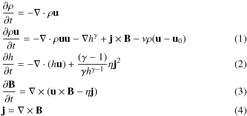
where, ρ,η, u, u₀, and B represent mass density, resistivity, plasma velocity, velocity of neutrals in the chromosphere, and magnetic field, respectively. The thermal pressure p is replaced by a proxy for the entropy h = (p/2)^1/γ, such that in the ideal limit (η → 0), the energy equation (Eq. (2)) takes a conservative form. The ratio of specific heats (γ) is taken to be 5/3 (adiabatic case).

All variables are normalized to typical system values and are, thus, dimensionless. The length scale, density, and magnetic field strength are normalized to typical values of L₀ = 500 km, ρ₀ = n₀m_p (where m_p is the proton mass and n₀ = 2.0 × 10¹⁵ m^-3), and B₀ = 1 × 10^-4 T, respectively. The pressure is measured in units of 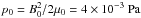${\mathit{p}}_{\mathrm{0}}\mathrm{=}{\mathit{B}}_{\mathrm{0}}^{\mathrm{2}}\mathit{/}\mathrm{2}{\mathit{\mu }}_{\mathrm{0}}\mathrm{=}\mathrm{4}\mathrm{\times }{\mathrm{10}}^{-3}\mathrm{Pa}$, while the velocity is normalized to a typical system Alfvén speed based on the normalizing magnetic field and plasma mass density 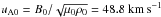${\mathit{u}}_{\mathrm{A}\mathrm{0}}\mathrm{=}{\mathit{B}}_{\mathrm{0}}\mathit{/}\sqrt{{\mathit{\mu }}_{\mathrm{0}}{\mathit{\rho }}_{\mathrm{0}}}\mathrm{=}\mathrm{48.8}\mathrm{km}\hspace{0.17em}{\mathrm{s}}^{-1}$. The timescale corresponds to the Alfvén transit time through the typical length scale τ_A = L₀/u_A = 10.25 s. Finally, the resistivity is normalized to η₀ = μ₀L₀ u_A0 = 3.066 × 10⁴ Ωm.

The plasma (flow velocity u) is coupled to the neutral gas (flow velocity u₀) in the chromosphere through collisions with a collision frequency denoted by ν. For simplicity, gravity, heat conduction, and radiative losses are not considered in the present study.

2.2. Numerical scheme

The simulations use a Leapfrog/DuFort-Frankel finite difference scheme that is second-order accurate and affords explicit control over dissipation (e.g., independent of grid resolution). While the Leapfrog scheme is free of dissipation (all even derivative terms cancel in the expansion), the DuFort-Frankel discretization, applied to the induction equation (Eq. (3)), introduces an explicit diffusion term. This term is consistent with the physical resistive diffusion term (ηj) in the induction equation. The method is accurate to second order with leading numerical diffusion, which varies as 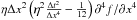$\mathit{\eta }\mathrm{\Delta }{\mathit{x}}^{\mathrm{2}}{}^{\mathrm{(}}\mathit{\eta }^{\mathrm{2}}\frac{\mathrm{\Delta }{\mathit{t}}^{\mathrm{2}}}{\mathrm{\Delta }{\mathit{x}}^{\mathrm{4}}}\mathrm{-}{\frac{\mathrm{1}}{\mathrm{12}}}^{\mathrm{)}}{\mathit{\partial }}^{\mathrm{4}}\mathit{f}\mathit{/}\mathit{\partial }{\mathit{x}}^{\mathrm{4}}$, such that the numerical diffusion is orders of magnitude smaller than the physical diffusion (controlled by the parameter η). These discretization methods are both three-step methods. It is thus necessary to employ an additional method in order to advance the simulation at the initial time step, thus generating the required two previous time levels. The Lax-Wendroff method (Potter 1973) is utilized for this initial iteration. This method exhibits the same numerical dispersion characteristics as the leapfrog method; however, whereas the leapfrog method was diffusionless, the Lax-Wendroff method introduces numerical diffusion that varies as Δx³.

The simulation domain is comprised of 259³ grid points and spans a region of 46.4 Mm in the (horizontal) x- and y-directions and 30.9 Mm in the (vertical) z-direction. The numerical grid is uniform in x and y with spacing Δ = 0.36 ( ~180 km), while the resolution in z is nonuniform, with a maximum resolution of Δz = 0.1 ( ~50 km) at the bottom of the simulation domain and a minimum resolution of Δz = 0.63 ( ~315 km) at the top boundary. The variation in grid spacing in z is displayed in Fig. 1. The grid is constructed to realize a higher resolution in z near the transition region from chromosphere to corona, where gradients of plasma parameters are largest.

To reduce numerical errors in the computation of the current density j, the magnetic field is separated into the initial current-free potential field (B₀) and the perturbed field (B_p) B = B₀ + B_p, such that ${j}\mathrm{=}\mathrm{\nabla }\mathrm{\times }{B}\mathrm{=}\mathrm{\nabla }\mathrm{\times }{{B}}_{\mathrm{p}}\mathit{.}$(5)The momentum equation (Eq. (1)) is implemented in this particular form (rather than the commonly used conservative expression) since it facilitates the expression of the current density according to Eq. (5), directly as ∇ × B_p, thus improving the accuracy of the computation of j (Santos et al. 2011).

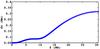Fig. 1 Illustration of the nonuniformity of grid spacing in the z-direction (dz). Z is the height above the photosphere.

2.3. Initial configuration

The initial magnetic field is generated from Fourier-filtered observations of the photospheric magnetic field in the vicinity of an X-ray bright point near the center of the solar disk. The line-of-sight (LOS) component of the photospheric magnetic field observed on December 19, 2006 at 22:17 UT by the Michelson Doppler Interferometer (MDI) aboard the SOHO spacecraft is Fourier-filtered, retaining only the first eight modes. This simplifies the magnetic structure of the system greatly and removes gradients on scales smaller than those resolvable by the current grid specifications. A potential magnetic field extrapolation according to Otto et al. (2007) is then applied to this Fourier-filtered photospheric magnetic field, thus rendering the desired magnetic structure for the simulation.

Though gravity is not considered in the current model, the atmosphere is defined in a stratified manner such that the transition region between the chromosphere and corona is approximated with a slightly enhanced width of ~1 Mm. To this end, the density is prescribed such that the chromospheric density is five orders of magnitude higher in the corona according to the equation $\mathit{\rho }\mathrm{\left(}\mathit{z}\mathrm{\right)}\mathrm{=}\frac{{\mathit{\rho }}_{\mathrm{chr}}}{\mathrm{2}}\left[\mathrm{1}\mathrm{-}\tanh \mathrm{\left(}\mathrm{2}\mathrm{\right(}\mathit{z}\mathrm{-}{\mathit{z}}_{\mathrm{0}}\mathrm{\left)}\mathrm{\right)}\right]\mathrm{+}{\mathit{\rho }}_{\mathrm{cor}}$(6)where ρ_chr and ρ_cor represent the chromospheric and coronal plasma densities, respectively. Initially, the transition region is centered at z₀ = 3 (1.5 Mm). The initial pressure is homogeneously set to unity throughout the simulation domain. According to the ideal gas law T = p/2k_Bn (where the factor of 2 arises from the consideration of the contribution from electrons as well as ions), yielding a temperature profile as shown together with the mass density in Fig. 2. The temperature is normalized to T₀ = p₀/2k_Bn₀ = 72   000 K, such that the initial coronal temperature is on the order of 10⁶ K.

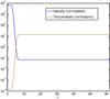Fig. 2 Height (z) profiles of normalized density and temperature.

Within the model, the plasma is driven by the motion of a neutral gas in the chromosphere. This photospheric flow is derived using the local correlation tracking (LCT) method, applied to the observed evolving photospheric magnetic field according to Santos et al. (2008). This motion is then approximated within the model through the inclusion of three incompressible vortices defined as $\begin{array}{ccc}{{u}}_{\mathrm{0}}\mathrm{=}\mathrm{\nabla }\mathrm{\times }\left[\frac{{\mathit{\phi }}_{\mathrm{0}}}{\cosh \mathrm{(}{\frac{\mathit{x}\mathrm{-}\mathit{y}\mathrm{+}{\mathit{c}}_{\mathrm{0}}}{{\mathit{l}}_{\mathrm{0}}}}^{\mathrm{)}}\cosh \mathrm{(}{\frac{\mathit{x}\mathrm{+}\mathit{y}\mathrm{+}{\mathit{d}}_{\mathrm{0}}}{{\mathit{l}}_{\mathrm{1}}}}^{\mathrm{)}}}\right]{ẑ}\mathit{.}& & \end{array}$The parameters of the vortices are chosen based on the observed quantities such that

• vortex 1:

  φ₀ = 0.1, c₀ = −18, d₀ = −102, l₀ = −12, l₁ = 12,

• vortex 2:

  φ₀ = 0.04, c₀ = 10, d₀ = −56, l₀ = −12, l₁ = 12,

• vortex 3:

  φ₀ = 0.11, c₀ = 38, d₀ = −76, l₀ = −14, l₁ = 14.

These normalized quantities result in a maximum horizontal photospheric speed of ~1.5 km   s^-1. The vortices employed in the simulation are shown in Fig. 3.

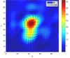Fig. 3 Illustration of the initial flow vortices (u0 in Eq. (1)) at the photospheric boundary along with the corresponding magnitude of the magnetic field (color-coded).

The chromospheric plasma is driven by this neutral flow through the height-dependent coupling term in the momentum equation (Eq. (1)). The height-dependence of this coupling coefficient ν(z) is chosen such that $\mathit{\nu }\mathrm{\left(}\mathit{z}\mathrm{\right)}\mathrm{=}\frac{{\mathit{\nu }}_{\mathrm{0}}}{\mathrm{2}}\left[\mathrm{1}\mathrm{-}\tanh \mathrm{\left(}\mathrm{20}\mathrm{\right(}\mathit{z}\mathrm{-}{\mathit{z}}_{\mathrm{c}}\mathrm{\left)}\mathrm{\right)}\right]\mathit{,}$(7)where the coupling coefficient ν₀ is taken to be 300 (about 30 s^-1). In Eq. (7), z_c defines the height at which the coupling effectively vanishes. For the simulation results presented here z_c = 0.254 (~125 km); i.e., the plasma and neutral gas are only coupled over the first few grid planes of the simulation domain.

2.4. Boundary conditions

The boundary conditions are prescribed in the manner laid out by Otto et al. (2007) so as to maintain consistency with the extrapolation scheme of the magnetic field and with the symmetry requirements of the MHD equations. To this end, the side boundaries employ line-symmetric boundary conditions, while the top and bottom boundaries use Neumann boundary conditions with $\frac{\mathit{\partial f}}{\mathit{\partial n}}{\mathrm{|}}_{{\mathit{z}}_{\min }\mathit{,}{\mathit{z}}_{\max }}\mathrm{=}\mathrm{0}$ on the physical boundary of the system. Additionally, the normal flow at the top and bottom boundaries is switched off, and B_n is defined through ∇·B = 0, while B_x and B_y are defined such that j_x = j_y = 0 at the bottom boundary.

3. Resistivity models

The aim of this work is to investigate of the effect of different resistivity models and parameterizations on the energization of bright points in the solar corona. To this end, a number of numerical simulations were carried out for various, micro-physically justified, resistivity models, implementing plausible parameters in order to study the reaction of the model corona driven by the same photospheric motion. We employed the classical Spitzer resistivity, similar to Spangler (2009), in a simulation that served to establish a reference for the subsequent models. This resistivity is based on classical transport theory and may be viewed as a plausible lower bound. The other simulations implemented anomalous resistivities based on macroscale models of kinetic instabilities.

3.1. Group 1: uniform and constant resistivity (η = const.) throughout the corona

In this group of simulations the resistivity was considered to be constant and uniform throughout the whole simulation domain. This approach is common in the literature. Results from simulation runs for two different resistivity values are presented here:

For reference, a constant resistivity was imposed at the level of the Spitzer resistivity $\mathit{\eta }\mathrm{=}\mathrm{5.2}\mathrm{\times }{\mathrm{10}}^{-5}\log \mathrm{\Lambda }\mathit{/}{\mathit{T}}_{\mathrm{e}}^{\mathrm{3}\mathit{/}\mathrm{2}}$. The Spitzer resistivity is very small in the corona, with a typical value of about 10^-10 (≈3 × 10^-6 Ωm) for T_e = 10⁶ K. The Spitzer value is chosen here for reference because it represents nearly ideal plasma conditions. The magnetic Reynolds number (R_m = μ₀ v ∗ L/η) may be expressed in terms of the normalized quantities as R_m = η₀/η, or simply 1/, where . Thus, the Spitzer resistivity of η = 10^-10 yields R_m = 10¹⁰.

A second set of simulations with a constant background resistivity was carried out with a higher value of η = 10^-3 (≈30 Ωm), as it is often assumed in the solar literature (see, e.g., Peter et al. 2006).

3.2. Group 2: variation in the coefficient of localized turbulent resistivity (η_eff)

Local resistivity may be effectively enhanced through turbulent dissipation resulting from the growth of current-driven micro-instabilities. The threshold for current and gradient drift instabilities may be formulated in terms of a critical drift velocity of the current carriers (Büchner & Elkina 2005). This can be taken into account within the simulation by comparing the current-carrier velocity v_cc = j/ne obtained from the macroscopic MHD plasma parameters with a critical value v_crit by applying additional anomalous (i.e., turbulent) resistivity when v_cc exceeds this critical value according to the relation 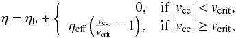$\mathit{\eta }\mathrm{=}{\mathit{\eta }}_{\mathrm{b}}\mathrm{+}\{\begin{array}{c}\\ \mathrm{0}\mathit{,}& \mathrm{if}\mathrm{\left|}{\mathit{v}}_{\mathrm{cc}}\mathrm{\right|}\mathit{<}{\mathit{v}}_{\mathrm{crit}}\mathit{,}\\ {\mathit{\eta }}_{\mathrm{eff}}\mathrm{(}\frac{{\mathit{v}}_{\mathrm{cc}}}{{\mathit{v}}_{\mathrm{crit}}}\mathrm{-}{\mathrm{1}}^{\mathrm{)}}\mathit{,}& \mathrm{if}\mathrm{\left|}{\mathit{v}}_{\mathrm{cc}}\mathrm{\right|}\mathrm{\ge }{\mathit{v}}_{\mathrm{crit}}\mathit{,}\end{array}$(8)where, η_eff is the coefficient that scales the effective anomalous resistivity, which is switched on locally where the condition | v_cc | > v_crit is fulfilled; and η_b denotes a constant background resistivity consistent with the Spitzer value as in the ideal plasma reference case of simulation Group 1, where η_b = 10^-10 (≈3 × 10^-6 Ωm). The threshold level in Eq. (8), v_crit, may be obtained through kinetic plasma theory, since it is on the kinetic scale that such micro-turbulence is generated. This is typically the ion inertial length scale c/ω_pi where, ${\mathit{\omega }}_{\mathrm{pi}}\mathrm{=}\sqrt{\mathit{n}{\mathit{e}}^{\mathrm{2}}\mathit{/}{\mathit{ϵ}}_{\mathrm{0}}{\mathit{m}}_{\mathit{i}}}$ is the ion plasma frequency (see, e.g., Büchner & Elkina 2006).

These scales are well below the resolution of the MHD simulations such that the current carrier velocity computed on the MHD grid level is always orders of magnitude lower than the critical threshold velocity. To include the onset of micro-turbulence requires either to assume that the simulation current density is concentrated on the subgrid scale of λ_i = c/ω_pi or, equivalently, to reduce the threshold velocity by the corresponding scale factor. Following the second approach replaces the ratio of v_cc/v_crit with v_cc/v_sim,crit where v_sim,crit is the critical threshold velocity obtained by expanding the critical current layer from the subgrid scale λ_i to the MHD grid scale.

The total critical current I_crit in the narrow layer leading to the onset of micro-turbulence is I_crit = λ_i|j_crit|. On the MHD grid, the macroscopic current density is computed at grid point i from magnetic field values at i + 1 and i − 1, where the spacing between grid points is Δ. Thus, current conservation yields $\left|{\mathit{j}}_{\mathrm{sim}\mathit{,}\mathrm{crit}}\right|\mathrm{2}\mathrm{\Delta }\mathrm{=}{\mathit{\lambda }}_{\mathit{i}}\left|{\mathit{j}}_{\mathrm{crit}}\right|\mathit{.}$(9)Correspondingly, the critical current carrier velocity determined on the macroscopic simulation grid scale is defined as v_sim,crit = |j_sim,crit|/${\mathrm{(}}^{}\mathit{n}{\mathit{e}}^{\mathrm{)}}$. Thus, Eq. (9) may be rewritten as

${\mathit{v}}_{\mathrm{sim}\mathit{,}\mathrm{crit}}\mathrm{=}\frac{{\mathit{\lambda }}_{\mathit{i}}}{\mathrm{2}\mathrm{\Delta }}{\mathit{v}}_{\mathrm{crit}}\mathit{.}$According to kinetic plasma theory, v_crit is typically some fraction of the electron thermal speed (${\mathit{v}}_{\mathrm{te}}\mathrm{=}\sqrt{{\mathit{k}}_{\mathrm{B}}{\mathit{T}}_{\mathrm{e}}\mathit{/}{\mathit{m}}_{\mathrm{e}}}$), v_crit = Cv_te, where C is usually a fraction of unity, depending on the particular type of instability excited (cf. Büchner & Daughton 2007). Defining the scale factor κ_i = λ_i/2Δ, the critical speed employed within the simulations is expressed as 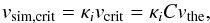${\mathit{v}}_{\mathrm{sim}\mathit{,}\mathrm{crit}}\mathrm{=}{\mathit{\kappa }}_{\mathit{i}}{\mathit{v}}_{\mathrm{crit}}\mathrm{=}{\mathit{\kappa }}_{\mathit{i}}\mathit{C}{\mathit{v}}_{\mathrm{the}}\mathit{,}$(10)thus providing the corresponding macroscopic threshold for the current carrier velocity on the numerical grid scale. The current carrier velocity on this scale is v_cc = j/ne, and in normalized simulation units the current carrier velocity and the critical velocity on the grid scale are given by the following relations: 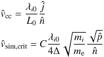$\begin{array}{ccc}& & \mathit{v̂}\mathrm{cc}\mathrm{=}\frac{{\mathit{\lambda }}_{\mathit{i}\mathrm{0}}}{{\mathit{L}}_{\mathrm{0}}}\frac{\mathit{ĵ}}{\mathit{n̂}}\\ & & \mathit{v̂}\mathrm{sim}\mathit{,}\mathrm{crit}\mathrm{=}\mathit{C}\frac{{\mathit{\lambda }}_{\mathit{i}\mathrm{0}}}{\mathrm{4}\mathrm{\Delta }}\sqrt{\frac{{\mathit{m}}_{\mathit{i}}}{{\mathit{m}}_{\mathrm{e}}}}\frac{\sqrt{\mathit{p̂}}}{\mathit{n̂}}\end{array}$with λ_i0 = c/ω_pi0, 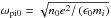${\mathit{\omega }}_{\mathrm{pi}\mathrm{0}}\mathrm{=}\sqrt{{\mathit{n}}_{\mathrm{0}}{\mathit{e}}^{\mathrm{2}}\mathit{/}{}^{\mathrm{(}}\mathit{ϵ}_{\mathrm{0}}{\mathit{m}}_{\mathit{i}}{}^{\mathrm{)}}}$ and the assumption k_BT_e = k_BT_i = p/2n. Therefore, the onset condition for a turbulent resistivity expressed on the MHD grid scale is 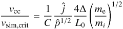$\frac{{\mathit{v}}_{\mathrm{cc}}}{{\mathit{v}}_{\mathrm{sim}\mathit{,}\mathrm{crit}}}\mathrm{=}\frac{\mathrm{1}}{\mathit{C}}\frac{\mathit{ĵ}}{\mathit{p̂}\mathrm{1}\mathit{/}\mathrm{2}}\frac{\mathrm{4}\mathrm{\Delta }}{{\mathit{L}}_{\mathrm{0}}}{\left(\frac{{\mathit{m}}_{\mathrm{e}}}{{\mathit{m}}_{\mathit{i}}}\right)}^{\mathrm{1}\mathit{/}\mathrm{2}}$(11)where the uniform gridspacing in x and y with Δ = 180 km is used. Equation (11) provides the macroscopic threshold for the current carrier velocity on the numerical grid scale including the factor C, which provides a means by which to set the particular threshold consistent with the relevant instability. It is important to note that this condition requires all of the MHD grid scale current to be concentrated on the ion inertia subgrid level and to fill the entire MHD grid cross section. Since this is not necessarily the case, the model will overestimate resistive diffusion and reconnection. It is also noted that the onset of resistivity only depends on the local current density and pressure in addition to the constant parameters in Eq. (11).

To avoid spatial and temporal discontinuities in the evolution of the parameter dependent resistivity resulting from Eq. (8), the distribution is first smoothed spatially, by averaging over the nearest-neighbor grid points (yielding ⟨ η ⟩ _x,y,z) and, then smoothed temporally in order to avoid instantaneous jumps, by advancing the distribution according to the following relation: $\mathit{\eta }\mathrm{(}\mathit{t}\mathrm{+}\mathrm{\Delta }\mathit{t}\mathrm{)}\mathrm{=}\mathit{\eta }\mathrm{\left(}\mathit{t}\mathrm{\right)}\mathrm{+}\mathrm{\Delta }\mathit{t}\mathrm{(}\mathrm{⟨}\mathit{\eta }{\mathrm{⟩}}_{\mathit{x,y,z}}\mathrm{(}\mathit{t}\mathrm{)}\mathrm{-}\mathit{\eta }\mathrm{(}\mathit{t}{\mathrm{\left)}}^{\mathrm{\right)}}\mathit{.}$(12)The simulations presented within Group 2 aim to investigate the influence of a locally enhanced resistivity according to Eq. (8) by using three values of the coefficient of anomalous resistivity: η_eff = 10^-3,10^-2, and 0.1 (corresponding to 30 Ωm, 300 Ωm, and 3000 Ωm), with C = 1/270. These values cover the range of anomalous resistivities previously obtained through kinetic simulations of gradient and current driven instabilities (cf. Silin et al. 2005; Büchner & Elkina 2006).

3.3. Group 3: variation in local thresholds (v_crit) for enhanced resistivity

While the cases of Group 2 investigated the influence of the coefficient of anomalous resistivity (η_eff) on the energization of the corona through current dissipation, given a singular critical value for the switch-on criterion (i.e., a current carrier velocity exceeding the electron thermal velocity multiplied by the factor C = 1/270), the simulations within Group 3 examine the influence of the switch-on threshold. Results presented here are for current carrier velocities that exceed the electron thermal velocity multiplied by factors C = 1/2.7, 1/270, and 1/2700. The same coefficient of effective resistivity η_eff = 10^-2 (300 Ωm) was applied in all cases of this group.

3.4. Group 4: constant thresholds for additional resistivity

In Group 4, the effect of a constant, uniform critical velocity was examined with the choice of v_crit = Cv_te,c; i.e., the onset velocity is chosen as a fraction of the typical electron thermal speed in the lower corona with T_e,c = 7 × 10⁵ K. Two cases with a very low constant critical onset velocity of v_sim,crit = 5 × 10^-4 m/s and a higher onset value of 5 × 10^-2 m/s are considered in this group. The scaling of the critical onset speed to the MHD grid scale is the same as in Eq. (10) but uses a typical coronal density of n_c = 10¹⁴ m^-3. This choice generates a velocity ratio for the onset of resistivity according to $\frac{{\mathit{v}}_{\mathrm{cc}}}{{\mathit{v}}_{\mathrm{sim}\mathit{,}\mathrm{crit}}}\mathrm{=}\frac{\mathrm{1}}{\mathit{C}}\frac{\mathit{ĵ}}{\mathit{n̂}}\frac{{\mathit{\omega }}_{\mathrm{pi}\mathit{,}\mathrm{c}}\mathrm{2}\mathrm{\Delta }}{{\mathit{\omega }}_{\mathrm{pi}\mathrm{0}}{\mathit{L}}_{\mathrm{0}}}\frac{{\mathit{u}}_{\mathrm{A}\mathrm{0}}}{{\mathit{v}}_{\mathrm{thec}}}$(13)with ${\mathit{v}}_{\mathrm{te}\mathit{,}\mathrm{c}}\mathrm{=}\sqrt{{\mathit{k}}_{\mathrm{B}}{\mathit{T}}_{\mathrm{e}\mathit{,}\mathrm{c}}\mathit{/}{\mathit{m}}_{\mathrm{e}}}$ and ${\mathit{\omega }}_{\mathrm{pi}\mathit{,}\mathrm{c}}\mathrm{=}\sqrt{{\mathit{n}}_{\mathrm{c}}{\mathit{e}}^{\mathrm{2}}\mathit{/}{}^{\mathrm{(}}\mathit{ϵ}_{\mathrm{0}}{\mathit{m}}_{\mathit{i}}{}^{\mathrm{)}}}$ for the condition v_cc ≥ v_sim,crit. This approach in effect removes the pressure dependence of the onset condition, which in Groups 2 and 3 entered via the thermal velocity v_te but introduces a dependence on the local plasma density. This choice of a constant threshold velocity corresponds to values of C = 2.4 × 10^-6 and 2.4 × 10^-4.

4. Results

All simulations were initialized with the same current free initial equilibrium configuration based on observations of a coronal bright point as discussed by Javadi et al. (2011). The initial magnetic structure is obtained through a potential field extrapolation of the first eight Fourier modes of the observed photospheric magnetic field (in accordance with Otto et al. 2007). This effectively removes the small-scale magnetic structures that are poorly resolved by the numerical grid. The resulting initial magnetic field is depicted in Fig. 4.

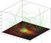Fig. 4 Illustration of the initial magnetic field extrapolated from the Fourier-filtered MDI magnetogram observations of the EUV bright point on December 19, 2006 at 22:17 UT. The magnetic field magnitude in the z = 0 plane is plotted in color, while the arrows in the z = 0 plane indicate the pattern of imposed photospheric motion.

The system is then driven by coupling the plasma to the inferred neutral gas motion within the chromosphere through the height-dependent collision profile given by Eq. (7). The resulting motion of the magnetic flux generates currents (Büchner 2006) with the potential to trigger locally enhanced resistivity, which can be described, for example, in accordance with Eq. (8).

To analyze the evolution of energy within the system, we calculate the kinetic (${\mathit{\epsilon }}_{\mathrm{kin}}\mathrm{=}{{}^{\mathrm{\int }}}_{\mathit{V}}\frac{\mathit{\rho }{\mathit{u}}^{\mathrm{2}}}{\mathrm{2}}\mathrm{d}\mathit{V}$), magnetic (${\mathit{\epsilon }}_{\mathrm{mag}}\mathrm{=}{{}^{\mathrm{\int }}}_{\mathit{V}}\frac{{\mathit{B}}^{\mathrm{2}}}{\mathrm{2}}\mathrm{d}\mathit{V}$) and thermal (${\mathit{\epsilon }}_{\mathrm{th}}\mathrm{=}{{}^{\mathrm{\int }}}_{\mathit{V}}\frac{\mathit{p}}{\mathrm{2}\mathrm{(}\mathit{\gamma }\mathrm{-}\mathrm{1}\mathrm{)}}\mathrm{d}\mathit{V}$) energies within the corona. To this end, the various contributions to the coronal energy budget are integrated over the simulation domain above the transition region, herein taken to be z = 3 (1500 km). Further, the MHD Eqs. (1)−(3) require the conservation of the sum of these three forms of energy. It is, thus, straightforward to express the temporal evolution of these three forms of energy within a given volume, directly from Eqs. (1)−(3): 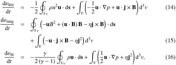$\begin{array}{ccc}\frac{\mathrm{d}{\mathit{\epsilon }}_{\mathrm{kin}}}{\mathrm{d}\mathit{t}}& \mathrm{=}& \mathrm{-}\frac{\mathrm{1}}{\mathrm{2}}{\mathrm{􏽉}}_{{\mathit{S}}_{\mathit{V}}}\mathit{\rho }{\mathit{u}}^{\mathrm{2}}{u}\mathrm{·}\mathrm{d}{s}\mathrm{+}{\mathrm{\int }}_{\mathit{V}}\left(\mathrm{-}\frac{\mathrm{1}}{\mathrm{2}}{u}\mathrm{·}\mathrm{\nabla }\mathit{p}\mathrm{+}{u}\mathrm{·}{j}\mathrm{\times }{B}\right){\mathrm{d}}^{\mathrm{3}}\mathit{v}\\ \frac{\mathrm{d}{\mathit{\epsilon }}_{\mathrm{mag}}}{\mathrm{d}\mathit{t}}& \mathrm{=}& 􏽉{\mathit{S}}_{\mathit{V}}\mathrm{(}\mathrm{-}{u}{\mathit{B}}^{\mathrm{2}}\mathrm{+}\mathrm{(}{u}\mathrm{·}{{B}}^{\mathrm{)}}{B}\mathrm{-}\mathit{\eta }{j}\mathrm{\times }{{B}}^{\mathrm{)}}\mathrm{·}\mathrm{d}{s}\\ & & \mathrm{+}{\mathrm{\int }}_{\mathit{V}}\mathrm{(}\mathrm{-}{u}\mathrm{·}{j}\mathrm{\times }{B}\mathrm{-}\mathit{\eta }{{j}}^{\mathrm{2}}\mathrm{)}{\mathrm{d}}^{\mathrm{3}}\mathit{v}\\ \frac{\mathrm{d}{\mathit{\epsilon }}_{\mathrm{th}}}{\mathrm{d}\mathit{t}}& \mathrm{=}& \mathrm{-}\frac{\mathit{\gamma }}{\mathrm{2}\left(\mathit{\gamma }\mathrm{-}\mathrm{1}\right)}{\mathrm{􏽉}}_{{\mathit{S}}_{\mathit{V}}}\mathit{p}{u}\mathrm{·}\mathrm{d}{s}\mathrm{+}{\mathrm{\int }}_{\mathit{V}}\left(\frac{\mathrm{1}}{\mathrm{2}}{u}\mathrm{·}\mathrm{\nabla }\mathit{p}\mathrm{+}\mathit{\eta }{{j}}^{\mathrm{2}}\right){\mathrm{d}}^{\mathrm{3}}\mathit{v}\mathit{.}\end{array}$The energy contribution from compression is expressed in Eqs. (14) and (16) in terms of the pressure (p) instead of h (as in Eq. (2)), since it is physically more intuitive to directly analyze the pressure gradient forces. Owing to the particular boundary conditions imposed on the simulation, there is, by definition, no net contribution to the energy flow from the surface integral terms at the side boundaries. Additionally, the contribution from the upper boundary is negligibly small. There is, however, a significant contribution from the inflow of energy through the lower boundary (z = 3) of the corona. As the main interest here is the investigation of the role of current dissipation in the energization of coronal plasma, we only consider processes within the volume defined as the corona, thus neglecting chromospheric contributions to the energy.

4.1. Group 1: uniform and constant resistivity (η = const.) throughout the corona

4.1.1. Almost ideal coronal plasma with η = 10^-10 (R_m = 10¹⁰)

To describe the evolution of a nearly ideal coronal plasma, the resistivity was prescribed uniformly throughout the domain such that η = 10^-10 (≈3 × 10^-6 Ωm). The resulting distributions of current density and current carrier velocities after 30 τ_A are illustrated by isosurfaces in Fig. 5.

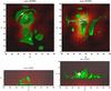Fig. 5 Isosurfaces of constant current density j = 5 (~10-3 A/m2) (left column) and of current carrier velocities j/n = 1 (or ~0.5 m/s) (right column) after 30 τA. The magnetic field strength is shown in red-orange, and the photospheric plasma flow velocities at the photospheric level are depicted by arrows.

The highest current densities develop below the transition region (see the left column of Fig. 5). These currents are dissipated effectively by collisional Spitzer resistivity, which is relatively strong in the actual chromosphere. It can thus be assumed that the dissipation of these currents effectively contributes to the heating of the chromosphere, which is not analyzed here. As the upper left plot shows, these currents occur in the chromosphere mainly in regions where the plasma motion strongly shears magnetically connected regions. Above the chromosphere the current densities are lower. Since the Spitzer resistivity in the corona is also small, the coronal currents are not efficiently dissipated by this mechanism.

The plots to the right of Fig. 5 display isosurfaces of the current carrier velocity j/n = 1 (or about 0.5 m/s in SI units). This plot clearly illustrates the extension of the potentially (micro-) turbulent regions, where current instabilities are expected to effectively enhance the resistivity and, therefore, cause Joule heating.

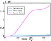Fig. 6 Temporal evolution of the thermal, kinetic, and magnetic energies within the corona above the transition region at z = 3 (1500 km) including the surface integrals in Eqs. (14)−(16).

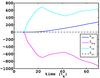Fig. 7 Temporal evolution of the thermal, kinetic, magnetic, and net energies within the volume above the transition region (neglecting inflow from the chromosphere).

Figure 6 illustrates the temporal evolution of the three forms of energy obtained by integrating Eqs. (14)−(16) through time within the simulated corona above the transition region at z = 3 (1500 km). The magnitude of the energies plotted in the figure (as well as similar plots throughout the remainder of this work) are measured in units of ${\mathit{E}}_{\mathrm{0}}\mathrm{=}{\mathit{B}}_{\mathrm{0}}^{\mathrm{2}}{\mathit{L}}_{\mathrm{0}}^{\mathrm{2}}\mathit{/}{\mathit{\mu }}_{\mathrm{0}}\mathrm{=}\mathrm{1}\mathrm{\times }{\mathrm{10}}^{\mathrm{15}}\mathrm{J}$. The curves in the figure represent the net change of energy, that is to say, the amount in excess of the initial values in the system at t = 0. In other words, Fig. 6 displays the evolution of the magnetic energy, which is added by the footpoint motion and the resulting Poynting flux as free energy to the pre-existing potential magnetic field. As the figure illustrates, this Poynting flux generated by the footpoint motion dominates the energy injection in the system. In fact, owing to the extremely low resistivity (η = 10^-10), the magnetic Reynolds number in this simulation is so large (10⁸) that Joule dissipation and magnetic reconnection (which would otherwise dissipate the accumulating magnetic energy) are rendered ineffective. The total amount of accumulated magnetic energy after 70 τ_A reaches Δε_mag = 1.9 × 10⁴ (1.9 × 10¹⁹ J). Also evident in Fig. 6 (as well as in the subsequent Figs. 7 and 8), is a delay of ~6.5 τ_A in the reaction of the corona to the onset of the photospheric driving. This is the time required by the Alvénic perturbation (due to the photospheric plasma motion) to propagate through the chromosphere to the base of corona and, thus, to the lower integration boundary.

To analyze the redistribution of energy contained within the corona between the kinetic, thermal, and magnetic components, only the volumetric contributions to the energy evolution within the corona (volume integrals in Eqs. (14)−(16)) are considered, discounting the energy inflow through the lower transition region. The resulting evolution of the different forms of energy are shown in Fig. 7. The figure clearly shows that both the kinetic and the thermal energy within the corona, grow at the expense of the magnetic field energy. The total amount of magnetic energy (δε_mag) transformed to thermal and kinetic energy within 70 τ_A (or 800 s) is ~900 (or 9 × 10¹⁷ J). This is only about 5% of the available free magnetic energy deposited throughout this interval to the corona. Figure 7 also illustrates that roughly two thirds of this magnetic energy is transformed to kinetic energy and approximately one third to thermal energy via plasma compression and Joule heating.

Monitoring the evolution of the energies according to Eqs. (14)−(16) allows the individual source terms within the corona to be analyzed. Figure 8 displays the contributions from these source terms for the Lorentz acceleration, compression, and Joule heating (i.e., for u·j   ×   B, $\frac{\mathrm{1}}{\mathrm{2}}{u}\mathrm{·}\mathrm{\nabla }\mathit{p}$, and ηj²), respectively, all measured in units of ${\mathit{\epsilon }}_{\mathrm{0}}\mathrm{=}{\mathit{v}}_{\mathrm{0}}{\mathit{B}}_{\mathrm{0}}^{\mathrm{2}}{\mathit{L}}_{\mathrm{0}}^{\mathrm{2}}\mathit{/}{\mathit{\mu }}_{\mathrm{0}}\mathrm{=}{\mathrm{10}}^{\mathrm{14}}\mathrm{W}$.

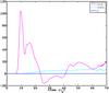Fig. 8 Temporal evolution of the volume integrated source terms ($\frac{\mathrm{1}}{\mathrm{2}}{u}\mathrm{·}\mathrm{\nabla }\mathit{p}$, u·j × B, and ηj2) according to Eqs. (14)−(16) in the corona above the transition region.

As previously indicated in Figs. 6 and 7, the initial perturbation generated by the motion of the plasma within the chromosphere takes about 6.5 τ_A to reach the lower boundary of the corona. This is consistent with the minimum chromospheric Alfvén transit time estimated from the maximum photospheric magnetic flux and plasma density. Coincidental with the arrival of the Alfvén waves at the transition region, the kinetic energy begins to increase due to Lorentz acceleration resulting from the growth of current sheets generated by these Alfvén waves in the lower corona. In the presence of significant resistivity, it is expected that the Joule heating would experience an analogous increase. However, such characteristics are not observed because of the extremely low Spitzer value utilized in this simulation. The subsequent evolution of the Lorentz force term (u·j × B) is governed by reflections of the Alfvén waves from the interface at the transition region subject to the continued driving of the footprints at the photospheric boundary. The initial Lorentz acceleration results in a compression of the overlying coronal plasma, as indicated by an increase in the $\frac{\mathrm{1}}{\mathrm{2}}{u}\mathrm{·}\mathrm{\nabla }{p}$ term at ~15 τ_A in Fig. 8 and a corresponding increase in thermal energy evident in Fig. 7. The front of the compressional wave launched into the corona can be seen in Fig. 9.

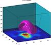Fig. 9 Illustration of the pressure wave generated by acceleration through Lorentz forces near the transition region. The surface encompasses the region within which the temperature is enhanced with respect to the initial coronal values.

This compression leads to a net thermal energy increase (see Fig. 7) of approximately 3 × 10¹⁷ J by ~70 τ_A.

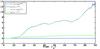Fig. 10 Temporal evolution of the thermal energy source terms ($\frac{\mathrm{1}}{\mathrm{2}}{u}\mathrm{·}\mathrm{\nabla }\mathit{p}$ and ηj2) within the volume above the transition region for two values of constant, uniform resistivity: η = 10-10 and η = 10-3.

For this case of low background resistivity, it is quite evident from the characteristics of the source terms in Fig. 8 that the net increase in thermal energy is almost entirely due to compressional heating affected through the $\frac{\mathrm{1}}{\mathrm{2}}{u}\mathrm{·}\mathrm{\nabla }\mathit{p}$ term, while heating due to current dissipation is negligible.

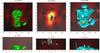Fig. 11 Isosurfaces showing (from left to right) regions of current density j ≥ 0.5 (8 × 10-5 A/m2), j/n ≥ 1 (i.e., a current carrier velocity vcc ≥ 0.5 m/s), and resistivity η ≥ 1 × 10-3 (30 Ωm) for the simulation run with a localized switch-on resistivity with ηeff = 0.01 after 30 τA. The magnetic field magnitude is shown in red-orange, and the flow at the photospheric boundary is illustrated by arrows.

4.1.2. Uniform coronal resistivity with η = 10^-3 (R_m = 10³)

Simulations were also carried out with a constant, uniform resistivity a factor of 10⁷ greater than the case just discussed, resulting in a small Reynolds number of R_m = 10³. Such high values of constant resistivity are typical in solar coronal simulations that support coronal heating through current dissipation. In Fig. 10, the resulting compressional and Joule heating source terms are shown for both the case of an almost ideal coronal plasma (η = 10^-10) and of the enhanced value of η = 10^-3. Consistent with the expectation noted in the previous section, the increased value of resistivity results in an increase in the Joule heating, concurrent with the arrival of the initial Alfvénic perturbation. Indeed, during the first 15 τ_A it dominates compression in generating thermal energy. After that time, however, the compressional contribution (which stays practically unchanged with respect to the ideal plasma case) again dominates the Joule heating, such that after 80 τ_A it is more than an order of magnitude larger. Considering that this is true despite the very large enhancement in resistivity (≈10⁷ × η_Spitzer), this implies that the currents extending into the corona are simply too weak to enable sufficient heating through Joule dissipation based on a model with a globally constant resistivity, even if such resistivity is taken to be extremely large.

4.2. Group 2: variation in the coefficient of localized turbulent resistivity (η_eff)

Results are presented in this section from a model utilizing a background resistivity identical to the one in the ideal case of the previous model (η_b = η_Spitzer), but with additional local enhancement based on Eqs. (12) and (8), with the critical velocity threshold for controlling the initialization of the anomalous resistivity given by Eq. (13) with C = 1/270.

To cover the range of anomalous resistivities previously obtained through kinetic simulations (cf. Silin et al. 2005; Büchner & Elkina 2006) we present results of simulations employing three different values for the coefficient of effective resistivity (η_eff) in Eq. (8): 10^-3,10^-2 and 0.1, which correspond to 30 Ωm, 300 Ωm, and 3000 Ωm.

Figure 11 depicts the spatial distribution of the current density, current carrier velocity, and resistivity at τ_A = 30 by means of appropriate isosurfaces of these quantities. The structure of the current density distribution is illustrated in the lefthand panel of the figure where the isosurfaces are drawn for a value of normalized current density one order of magnitude lower than those chosen in Fig. 5, i.e. for j = 0.5 or 10^-5 A/m². The locations of these current density enhancements correspond well with similar structures displayed in the lefthand column of Fig. 5 (for the case of a small background resistivity), indicating regions where plasma motion shears magnetically connected regions of the solar atmosphere. Owing to the locally enhanced resistivity, the magnitude of these currents is much lower than in the previous case with a constant background resistivity. The middle pane in Fig. 11 displays the spatial structure of the current carrier speed (| j | /n) illustrating the extent of the current density enhancements into the low-density corona. The pane on the right illustrates the region of enhanced resistivity enclosed by the surface defined as η ≥ 1 × 10^-3 (30 Ωm). Though the currents of largest magnitude develop within the chromosphere, they also extend into the lower corona (as illustrated in the center pane of the figure). Thus, defining the anomalous resistivity according to Eqs. (8) and (13) allows for the description of anomalous resistivity within the corona, as well as the chromosphere. The evolution of the various forms of energy, as well as the source terms themselves are displayed in Figs. 12 and 13, respectively.

Figure 12 indicates that the evolution of the kinetic energy is essentially the same as in the ideal plasma reference case with constant resistivity (Group 1). The enhanced local resistivity, however, makes the Joule heating contribution much stronger, and consequently, also the reduction in magnetic field energy. The magnetic gradients are reduced with enhanced current dissipation due to the locally increased effective resistivity, resulting in a significantly more stable simulation which is capable of evolving the system on a much larger time scale. This allows for examining the long term evolution of the system, while providing for a direct comparison of the results for the first ~70 τ_A of the results with those of Group 1 (see Figs. 7 and 8).

Figure 12 illustrates very similar behavior in terms of the magnetic and kinetic energies with respect to the results from Group 1. However, including the additional resistivity results in more rapid growth in thermal energy. Figure 13 shows the temporal evolution of the source terms $\frac{\mathrm{1}}{\mathrm{2}}{u}\mathrm{·}\mathrm{\nabla }\mathit{p}$, u·j × B, and ηj². Here again, after the initial Alfvénic perturbation reaches the transition region, strong currents are generated that accelerate the plasma through Lorentz forces. But, due to the local enhancement of resistivity, this current is dissipated through Joule heating. Thus, magnetic energy is more efficiently converted into thermal energy through magnetic diffusion. This simultaneously reduces the current density, and similarly the Lorentz force. This behavior is clear in Fig. 13: upon the arrival of the initial Aflvén waves at the transition region, there is a significant increase in both the v·(j × B) and v·∇(p/2) terms. Owing to the enhanced resistivity, the current is dissipated and the Lorentz force is reduced (approximately half that in the previous case). Additionally, plasma acceleration by the Lorentz force evolves more smoothly, whereas for the nearly ideal case, this acceleration is significantly more dynamic by exhibiting large-scale fluctuations on relatively short timescales thanks to the large magnitude of the thin current sheets which evolve in the ideal limit. Approximately 10 − 15 τ_A after the arrival of the initial perturbation, the magnetic energy within the enhanced current sheet has largely been converted into thermal energy. An apparent equilibrium is reached between the convective motion in the photosphere, which generates the currents and the Joule dissipation, which in turn converts magnetic energy into thermal, thus resulting in a relatively constant heating rate until ~70 τ_A. The resulting thermal energy at 70 τ_A is therefore approximately twice what is obtained in the results of Group 1 with a constant Spitzer resistivity. The heating rate, however, does not remain constant, and after ~80 τ_A the Joule heating continues to increase roughly linearly.

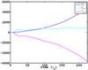Fig. 12 Temporal evolution of the thermal, kinetic, and magnetic energies for a localized switch-on resistivity with ηeff = 0.01 within the corona above the transition region.

The compression is nearly unchanged in comparison to the ideal plasma case of Group 1, at least over the first 70 τ_A where the former simulation was terminated (cf. Fig. 8). While the Joule heating term is enhanced due to the consideration of localized resistivity, it still never exceeds the compressional contribution to the energization of the corona.

To investigate the effect of the magnitude of the effective resistivity coefficient η_eff in Eq. (8), the temporal evolution of the compressional and Joule heating source terms is shown in Fig. 14. In addition to the results already presented in Fig. 12 for an effective resistivity of η_eff = 0.01 (300 Ωm), results are also displayed for simulations utilizing two additional values of the effective resistivity coefficient: η_eff = 0.1 (3 × 10³ Ωm) and 10^-3 (30 Ωm). The dashed lines in the figure depict the evolution of the compressional heating term, while the solid lines represent the Joule heating.

A comparison of the simulation results for different η_eff indicates that the early Joule heating, which occurrs when the Alfvén wave initially reaches the transition region, strongly depends on the resistivity coefficient, such that the maximum Joule heating rate for the case of η_eff = 0.1 (3 × 10³ Ωm) is more than twice that of the case previously discussed in which η_eff = 0.01 (3 × 10² Ωm), and more than a factor of 7 higher than for the case with η_eff = 10^-3 (30 Ωm). However, in the later evolution, all results exhibit a tendency for the compression to overtake the Joule heating as the dominant source driving thermal energy increase in the system, with the time at which this transition occurs increasing as a function η_eff. It should be noted that the higher values of η_eff are enhanced far beyond those justifiable within existing kinetic theories, requiring extraordinarily strong plasma turbulence, yet the compressional energization still exceeds the Joule heating (cf. also Fig. 13).

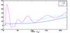Fig. 13 Temporal evolution of the volume integrated source terms ($\frac{\mathrm{1}}{\mathrm{2}}{u}\mathrm{·}\mathrm{\nabla }\mathit{p}$, u·j × B, and ηj2) within the corona above the transition region for an anomalous resistivity model described by Eqs. (8) and (13) with ηeff = 0.01 and vcrit = vte/270.

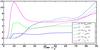Fig. 14 Temporal evolution of the compressional ($\frac{\mathrm{1}}{\mathrm{2}}{u}\mathrm{·}\mathrm{\nabla }\mathit{p}$) and Joule dissipation (ηj2) source terms within the corona above the transition region for three values of the local enhancement of the resistivity ηeff.

4.3. Group 3: variation in local thresholds (v_crit,kinetic) for enhanced resistivity

Since the onset of turbulent dissipation depends on the current carrier velocity threshold, a number of simulations were also carried out to examine the effect of the variation in this critical value leading to the onset of anomalous resistivity. The simulation results presented within this group represent variations in v_crit,kinetic given by the electron thermal speed reduced by a factor C of 1/2.7, 1/270 (for comparison with the previous group) and 1/2700. The effective resistivity coefficient was taken as η_eff = 0.01 (300 Ωm). Figure 15 directly compares the results for C = 1/2.7 (blue line) and 1/2700 (red line), as well as the reference case from Group 2 in which C = 1/270 (green line) for comparison.

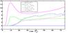Fig. 15 Temporal evolution of the source terms ($\frac{\mathrm{1}}{\mathrm{2}}{u}\mathrm{·}\mathrm{\nabla }\mathit{p}$ and ηj2) within the corona above the transition region for three values of the critical current carrier velocity C = 1/2.7 (blue lines), 1/270 (green lines), and 1/2700 (red lines).

Similar to results from Group 2, the early Joule heating rate shows a significant dependence on the magnitude of the critical value, with the resulting maximum Joule heating rate for the low critical value of C = 1/2700, more than a factor of 2.5 higher than for the reference parameter dependent case with C = 1/270. However, with such a low critical value of C = 1/2700, Joule heating becomes the dominant source of thermal energy increase throughout the simulation, heating at a rate roughly twice that because of compression from approximately 30 τ_A. The solid lines in Fig. 15 again depict the evolution of the Joule heating term, while dashed lines correspond to the compressional increase in the thermal energy in the corona. The simulation with the highest critical value C = 1/2.7 clearly shows that, for such a high threshold, the current carrier velocity never exceeds the critical value, and thus, the resulting thermal energy increase is entirely due to compressional heating. In the more realistic case of a critical switch-on threshold at the level of C = 1/270 (already discussed within Group 2), the compressional heating remains dominant over Joule heating. Only if the switch-on threshold is lowered to levels far below those justifiable by existing kinetic theories is the rate of Joule heating able to reach levels above that from compression.

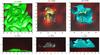Fig. 16 Isosurfaces showing (from left to right) regions of current density j ≥ 0.5 (8 × 10-5 A/m2), j/n ≥ 0.5 (current carrier velocity vcc ≥ 0.25 m/s), and resistivity η ≥ 1 × 10-3 (30 Ωm) for the simulation run with a constant and uniform switch-on criterion corresponding to a current carrier velocity of vcc = 1 × 10-6 (5 cm/s) after 20 τA. The magnetic field magnitude is shown in red-orange, and the flow at the photospheric boundary is illustrated by arrows.

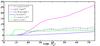Fig. 17 Temporal evolution of the source terms governing the thermal energy of the corona $\frac{\mathrm{1}}{\mathrm{2}}{u}\mathrm{·}\mathrm{\nabla }\mathit{p}$ (dashed lines) and ηj2 (solid lines) above the transition region for two uniform values of the critical switch-on thresholds corresponding to C = 2.4 × 10-4 (blue lines) and C = 2.4 × 10-6 (magenta lines) based on a coronal temperature of T = 106 K. For comparison, the reference case with a local coronal temperature dependent threshold value corresponding to C = 3.7 × 10-3 (green lines) is also shown.

4.4. Group 4: constant thresholds for additional resistivity

The simulations that comprise Group 4 investigate the effects of varying the critical threshold of the current carrier velocity (v_crit), but with a homogeneous value throughout the simulation domain. Two sets of results are presented herein, corresponding to v_crit ≈ 0.6 × 10^-3 m/s and 0.06 m/s. Based on typical values within the coronal model where T_cor = 10⁶ K and n_cor = 10¹⁴ m^-3, these values may be expressed (as in the previous group of simulations) as v_crit = Cv_te, where C = 2.4 × 10^-6 and C = 2.4 × 10^-4, respectively. Here, again, η_eff = 10^-2 (300 Ωm).

According to Eq. (8), the anomalous resistivity is only initialized when the current carrier velocity (v_cc = j/ne) rises above the critical value governed by Eq. (11). Thus, for the simulations that comprise Groups 2 and 3, the onset of anomalous resistivity tends to favor regions where enhanced current density is collocated with relatively low plasma pressure. This may be seen more directly through examining Eq. (11). However, by defining v_crit = C v_te, where C is a constant, the pressure dependence is removed and Eq. (11) becomes Eq. (13). Thus, the implementation of a constant critical value results in the onset of anomalous resistivity in locations where enhanced current density is collocated with low plasma density (i.e., within the corona). Consequently, whereas the parameter-dependent models of Groups 2 and 3 effectively generated anomalous resistivity in regions where the current density was highest (i.e., within the chromosphere since, initially, p = 1 throughout the simulation domain), the treatment of the resistivity within Group 4 favors the growth of anomalous resistivity where current sheets extend into the corona.

Figure 16 again displays isosurfaces encompassing regions of enhanced current density, current carrier velocity and resistivity. The highest current concentrations again develop within the chromosphere. These chromospheric current sheets are significantly more volume-filling than in the previous case, since, particularly in the absence of anomalous resistivity, there is no means by which to dissipate them (due to the inverse dependence of the turbulence induced η on the plasma density). Conversely, the resistivity (shown in the right pane of the figure) develops above the transition region in the locations where the current carrier velocity exceeds the critical parameter (middle pane of the figure). Thus, the distribution of enhanced resistivity, and as a result, Joule dissipation is effectively restricted to the volume defined by the corona.

Figure 17 again displays the temporal evolution of the source terms for the cases of C = 2.4 × 10^-6 and C = 2.4 × 10^-4. For comparison with the model incorporating a local coronal temperature and density dependent threshold, results are shown again for the reference case with C = 1/270.

As illustrated in Fig. 17, neither of the simulations that rely on a uniform value for the critical parameter exhibits the early jump in Joule heating characteristic of all results discussed previously (also evident in Fig. 17 again for the reference case) around 8 τ_A. Rather, for the cases discussed here, the Joule heating realizes a comparatively gradual rise, beginning at ~10 τ_A and 20 τ_A for the cases of C = 2.4 × 10^-6 and C = 2.4 × 10^-4, respectively. This is a result of the inverse dependence of the resistivity on the plasma density; as the initial Alfvén wave reaches the transition region, the local density is still quite high, and thus, the current carrier velocity remains below the critical value, realizing a comparable magnitude more gradually with increasing height into the corona.

While the evolution of the compressional energization only weakly depends on the choice of the critical threshold velocity for the anomalous resistivity, the Joule heating exhibits a more significant dependence. However, only in the unrealistic case, with an extremely low threshold corresponding to C = 2.4 × 10^-6, does the Joule heating dominate the energization through compression, ultimately reaching a value about five times higher than the compressional heating by the end of the simulation (75 τ_A, cf. Fig. 17). The results for a more realistic critical value that is two orders of magnitude higher exhibit the inverse behavior: the energization of the coronal plasma is dominated by compression that is more than twice as large, however, the critical velocity corresponding to this threshold is less than 1 mm/s. This is completely unrealistic in terms of an anomalous resistivity arising from current or gradient instabilities driven by micro-turbulence. Even the higher critical threshold value corresponding to C = 2.4 × 10^-4 (i.e., a current carrier velocity j/ne of a few cm/s) is still unrealistically low to generate significantly enhanced Joule heating that could dominate compression in heating the coronal plasma, suggesting that the role of local Joule dissipation associated with the bright point is insignificant in driving coronal energization.

5. Summary and discussion

We have presented results from numerical simulations that investigate the consequences of various modifications to the resistivity model on the role of Joule dissipation versus compressional heating in the evolution of thermal energy within the solar corona. The particular configuration presented is the quiet solar corona in the vicinity of a solar coronal X-ray bright point observed on December 19, 2006 at 22:17 UT. The various resistivity models considered here have been separated into four groups that may be summarized as follows:

• 1.

  A constant and homogeneous resistivity with particu-lar values corresponding to the Spitzer resistivity basedon typical parameters within the model corona yieldingη ≈ 3 × 10^-6 Ωm, in addition to an enhanced value of η ≈ 3 × 10^-3 Ωm. The magnetic Reynolds number corresponding to the former is then R_m = 10¹⁰ (resulting in nearly ideal plasma conditions).

• 2.

  A current carrier velocity dependent resistivity according to Eq. (8) in which the effective resistivity coefficient η_eff was varied, while the critical current carrier velocity threshold (in terms of the local electron thermal velocity) was kept constant.

• 3.

  A current carrier velocity dependent resistivity according to Eq. (8), in which the ratio of the critical value v_crit to the local electron thermal velocity was varied, while the effective resistivity coefficient η_eff was kept constant.

• 4.

  Two cases of a current carrier velocity dependent resistivity according to (8), but with the critical value (v_crit) set to a constant and uniform value throughout the domain (i.e., not depending on the local plasma temperature enhancement).

These numerical investigations into the distribution of energy in a quiet, driven solar corona indicate, qualitatively, that the large-scale coronal dynamics are largely unaffected by changes to the resistivity model. The same Poynting flux is injected into the system through the photospheric plasma motion driving the chromospheric plasma, which is collisionally coupled to the inferred photospheric neutral motion. This increases the magnetic energy in the corona, which is subsequently converted through Joule dissipation and plasma acceleration due to the Lorentz force into thermal and kinetic energy, respectively. In particular we conclude that

• For lower threshold values (C = v_crit/v_te) the anomalous resistivity is initiated earlier and develops over a larger spatial extent, thus resulting in a greater total Joule dissipation.

• A larger effective resistivity coefficient (η_eff) leads to more Joule dissipation.

• Compressional heating exhibits only a weak dependence on the resistivity model.

The results of the variation in the resistivity models are in general agreement with those from the similar 2D reconnection work of Roussev et al. (2002). However, our results further imply that the energization of the solar corona is dominated by the plasma compression due to Lorentz forces caused by the plasma motion at the photospheric boundary. Only for resistivity parameters that are extreme overestimates (i.e., for a critical current carrier velocity < 1 mm/s in Group 4, or for v_crit = v_the/2700 in Group 3) does the Joule dissipation begin to dominate the thermal energy increase in the corona. Thus, our findings extend the results of Javadi et al. (2011) and Santos et al. (2011) to a system with higher resolution.

To accurately address the physical processes related to magnetic dissipation within the framework of resistive MHD, one must choose an appropriate resistivity for the system under consideration. The significance of this parameter may be understood through examining the induction equation (Eq. (3)). The magnetic Reynold’s number (R_m) is the ratio of the magnitude of the convective term to the dissipative term

${\mathit{R}}_{\mathrm{m}}\mathrm{=}\frac{\mathrm{|}\mathrm{\nabla }\mathrm{\times }\mathrm{(}{u}\mathrm{\times }{B}\mathrm{\left)}\mathrm{\right|}}{\mathrm{\left|}\mathit{\eta }{\mathrm{\nabla }}^{\mathrm{2}}{B}\mathrm{\right|}}\mathit{,}$or

${\mathit{R}}_{\mathrm{m}}\mathrm{=}\frac{\mathit{uL}}{\mathit{\eta }}\mathit{,}$where u and η represent local velocity and resistivity, while L indicates the typical length scale over which parameters realize a significant gradient. Thus, R_m ≫ 1 implies that the magnetic field evolves thanks to convective motions of the plasma, while R_m ≪ 1 implies that dissipation of the magnetic field occurs on timescales faster than convective processes. Typically, solar plasma is characterized by R_m ≫ 1; however, on small scales (i.e., resistive layers) it is expected that the magnitude of the dissipative term becomes comparable to that of the convective term, such that R_m ≈ 1. The important point here is that specifying a value of η, in turn, defines a length scale on which diffusive processes become comparable to convection. In other words, If the resistivity is chosen extremely low (, for instance), then, requiring R_m = 1 for a plasma flow speed that is typical of the simulations (), yields a dissipation length scale: $\begin{array}{ccc}{\mathit{l}}_{\mathrm{diss}}& \mathrm{=}& \frac{\mathit{\eta ̂}}{\mathit{v̂}}{\mathit{L}}_{\mathrm{0}}\\ & \mathrm{\approx }& \mathrm{2.5}\mathrm{cm}\mathit{.}\end{array}$This is significantly less than the grid resolution of ~50 km. Thus, the simulation underestimates the Joule dissipation for current sheets that would collapse to such a small scale. However, this simulation employing the Spitzer resistivity is intended only to serve as a nearly ideal reference for the cases that follow. A similar analysis of the second case of Group 1 yields a dissipation length scale of ≈25 km, which is just at the limit of the grid resolution. These estimates of the dissipation scale length are based on a particular plasma velocity, and it should be noted that this quantity varies widely throughout the simulation domain. Thus, because of the inverse relationship between the scale length and the plasma flow magnitude, the dissipation scale length can be much greater than those calculated above.

The implementation of an anomalous resistivity model, as employed in the remaining simulations, allows for a much enhanced value of the resistivity within a limited region and a similar increase in the dissipation scale. For instance, the resistivity in the simulation of Group 2 with η_eff = .01 reaches values of , where local plasma velocity is . These conditions yield a local dissipation scale of l_diss = 2 Mm, which is easily resolved by at least ten grid points.

The Joule dissipation realized in the simulations is likely to be overestimated due to the scaling factor $\frac{\mathrm{1}}{\mathrm{2}\mathrm{\Delta }}\frac{\mathit{c}}{{\mathit{\omega }}_{\mathrm{pi}}}$, and thus, should be viewed as an upper bound to the actual dissipation occurring in the solar atmosphere. Though this expansion factor ensures conservation of the total surface current through a current sheet cross-section, the corresponding region over which the anomalous resistivity may develop is much more expansive than that expected in the physical system.

Gudiksen & Nordlund (2005), as well as Peter et al. (2006), have argued that Joule dissipation may play a primary role in the heating of the corona. We note here, however, that while the respective authors illustrate the importance of Joule heating by numerical simulation, they also indicate that the majority of this heating (approximately 90% of the total energy dissipation in the case of the former) occurs within the chromosphere. Our results appear, at least qualitatively, to agree with such a localization of the Joule dissipation. The analysis of the energy distribution within the system presented here draws a clear distinction between the corona and the chromosphere, with the ensuing discussion focusing on energy conversion within the limited volume above the solar transition region, namely, the corona. Although we have not directly analyzed the energy conversion within the chromosphere in our model, we note that the most significant currents lie well below the transition region (see Figs. 5 and 11), and they are rather extensive in terms of spatial distribution. As a result, it may be expected that Joule dissipation plays a far more important role in the energization of the chromosphere than in the corona. We have, instead, limited our discussion to processes within the corona, because of the simplified treatment of the coupling of the chromospheric plasma to the inferred inferred convection of the chromospheric neutral population (through the last term on the righthand side of the momentum equation, see Eq. (1)). A more complete description of the chromosphere would require a multifluid approach in order to give full consideration to the effects of ionization, recombination, and energy exchange.

Thus, the apparent disagreement between our results and those of Gudiksen & Nordlund (2005) and Peter et al. (2006)

may be attributable to differing definitions of the corona within the respective models. However, our results also demonstrate that the ratio of Joule to compressional heating depends very much on the chosen resistivity model. Models that are more accurately representative of the physical conditions generate significantly less Joule dissipation and compressional heating generally dominates in these models. The use of a much higher resistivity is in ours, as in other works, motivated by the limited resolution and the assumption that the actual current is indeed localized on the dissipation (subgrid) scale and fills the entire cross-sectional area of a grid cell. However, this is certainly not always the case, such that the presented results, as well as other results in the literature on Ohmic dissipation in coronal simulations, should rather be considered as an upper limit that is likely orders of magnitude too high.

Our results indicate that it is, of course, possible to generate a system in which thermal energy increase is largely driven by direct Joule dissipation, providing a sufficiently high resistivity is assumed. A more conservative and physically justified approach leads us to conclude that compression is the dominant source of plasma energization in the quiet solar corona.

Acknowledgments

The authors are grateful to the Max-Planck Society for funding parts of this work by the Interinstitutional Research Initiative “Turbulent transport and ion heating, reconnection and electron acceleration in solar and fusion plasmas” Project No. MIF-IF-A-AERO8047.

References

All Figures

	Fig. 1 Illustration of the nonuniformity of grid spacing in the z-direction (dz). Z is the height above the photosphere.
In the text

	Fig. 2 Height (z) profiles of normalized density and temperature.
In the text

	Fig. 3 Illustration of the initial flow vortices (u0 in Eq. (1)) at the photospheric boundary along with the corresponding magnitude of the magnetic field (color-coded).
In the text

	Fig. 4 Illustration of the initial magnetic field extrapolated from the Fourier-filtered MDI magnetogram observations of the EUV bright point on December 19, 2006 at 22:17 UT. The magnetic field magnitude in the z = 0 plane is plotted in color, while the arrows in the z = 0 plane indicate the pattern of imposed photospheric motion.
In the text

	Fig. 5 Isosurfaces of constant current density j = 5 (~10-3 A/m2) (left column) and of current carrier velocities j/n = 1 (or ~0.5 m/s) (right column) after 30 τA. The magnetic field strength is shown in red-orange, and the photospheric plasma flow velocities at the photospheric level are depicted by arrows.
In the text

	Fig. 6 Temporal evolution of the thermal, kinetic, and magnetic energies within the corona above the transition region at z = 3 (1500 km) including the surface integrals in Eqs. (14)−(16).
In the text

	Fig. 7 Temporal evolution of the thermal, kinetic, magnetic, and net energies within the volume above the transition region (neglecting inflow from the chromosphere).
In the text

	Fig. 8 Temporal evolution of the volume integrated source terms ($\frac{\mathrm{1}}{\mathrm{2}}{u}\mathrm{·}\mathrm{\nabla }\mathit{p}$, u·j × B, and ηj2) according to Eqs. (14)−(16) in the corona above the transition region.
In the text

	Fig. 9 Illustration of the pressure wave generated by acceleration through Lorentz forces near the transition region. The surface encompasses the region within which the temperature is enhanced with respect to the initial coronal values.
In the text

	Fig. 10 Temporal evolution of the thermal energy source terms ($\frac{\mathrm{1}}{\mathrm{2}}{u}\mathrm{·}\mathrm{\nabla }\mathit{p}$ and ηj2) within the volume above the transition region for two values of constant, uniform resistivity: η = 10-10 and η = 10-3.
In the text

Fig. 11 Isosurfaces showing (from left to right) regions of current density j ≥ 0.5 (8 × 10-5 A/m2), j/n ≥ 1 (i.e., a current carrier velocity vcc ≥ 0.5 m/s), and resistivity η ≥ 1 × 10-3 (30 Ωm) for the simulation run with a localized switch-on resistivity with ηeff = 0.01 after 30 τA. The magnetic field magnitude is shown in red-orange, and the flow at the photospheric boundary is illustrated by arrows.

In the text

	Fig. 12 Temporal evolution of the thermal, kinetic, and magnetic energies for a localized switch-on resistivity with ηeff = 0.01 within the corona above the transition region.
In the text

	Fig. 13 Temporal evolution of the volume integrated source terms ($\frac{\mathrm{1}}{\mathrm{2}}{u}\mathrm{·}\mathrm{\nabla }\mathit{p}$, u·j × B, and ηj2) within the corona above the transition region for an anomalous resistivity model described by Eqs. (8) and (13) with ηeff = 0.01 and vcrit = vte/270.
In the text

	Fig. 14 Temporal evolution of the compressional ($\frac{\mathrm{1}}{\mathrm{2}}{u}\mathrm{·}\mathrm{\nabla }\mathit{p}$) and Joule dissipation (ηj2) source terms within the corona above the transition region for three values of the local enhancement of the resistivity ηeff.
In the text

	Fig. 15 Temporal evolution of the source terms ($\frac{\mathrm{1}}{\mathrm{2}}{u}\mathrm{·}\mathrm{\nabla }\mathit{p}$ and ηj2) within the corona above the transition region for three values of the critical current carrier velocity C = 1/2.7 (blue lines), 1/270 (green lines), and 1/2700 (red lines).
In the text

Fig. 16 Isosurfaces showing (from left to right) regions of current density j ≥ 0.5 (8 × 10-5 A/m2), j/n ≥ 0.5 (current carrier velocity vcc ≥ 0.25 m/s), and resistivity η ≥ 1 × 10-3 (30 Ωm) for the simulation run with a constant and uniform switch-on criterion corresponding to a current carrier velocity of vcc = 1 × 10-6 (5 cm/s) after 20 τA. The magnetic field magnitude is shown in red-orange, and the flow at the photospheric boundary is illustrated by arrows.

In the text

Fig. 17 Temporal evolution of the source terms governing the thermal energy of the corona $\frac{\mathrm{1}}{\mathrm{2}}{u}\mathrm{·}\mathrm{\nabla }\mathit{p}$ (dashed lines) and ηj2 (solid lines) above the transition region for two uniform values of the critical switch-on thresholds corresponding to C = 2.4 × 10-4 (blue lines) and C = 2.4 × 10-6 (magenta lines) based on a coronal temperature of T = 106 K. For comparison, the reference case with a local coronal temperature dependent threshold value corresponding to C = 3.7 × 10-3 (green lines) is also shown.

In the text

References

- Bárta, M., Büchner, J., Karlický, M., & Skála, J. 2011, ApJ, 737, 24 [NASA ADS] [CrossRef] [Google Scholar]
- Bhattacharjee, A., & Yuan, Y. 1995, ApJ, 449, 739 [NASA ADS] [CrossRef] [Google Scholar]
- Büchner, J. 2006, Space Sci. Rev., 122, 149 [NASA ADS] [CrossRef] [Google Scholar]
- Büchner, J., & Daughton, W. 2007, Reconnection of magnetic fields: magnetohydrodynamics and collisionless theory and observations (Cambridge University Press), 144 [Google Scholar]
- Büchner, J., & Elkina, N. V. 2005, Space Sci. Rev., 121, 237 [NASA ADS] [CrossRef] [Google Scholar]
- Büchner, J., & Elkina, N. 2006, Phys. Plasmas, 13, 082304 [NASA ADS] [CrossRef] [Google Scholar]
- Büchner, J., Nikutowski, B., & Otto, A. 2004a, in SOHO 15 Coronal Heating, eds. R. W. Walsh, J. Ireland, D. Danesy, & B. Fleck, ESA SP, 575, 23 [Google Scholar]
- Büchner, J., Nikutowski, B., & Otto, A. 2004b, in Multi-Wavelength Investigations of Solar Activity, eds. A. V. Stepanov, E. E. Benevolenskaya, & A. G. Kosovichev, IAU Symp., 223, 353 [Google Scholar]
- Büchner, J., Nikutowski, B., & Otto, A. 2005, in Particle Acceleration in Astrophysical Plasmas: Geospace and Beyond, eds. D. Gallagher, J. Horwitz, J. Perez, R. Preece, & J. Quenby (Washington DC.: AGU), AGU monograph, 156, 161 [Google Scholar]
- Démoulin, P. 2006, Adv. Space Res., 37, 1269 [NASA ADS] [CrossRef] [Google Scholar]
- Gudiksen, B. V., & Nordlund, Å. 2005, ApJ, 618, 1020 [NASA ADS] [CrossRef] [Google Scholar]
- Habbal, S. R., & Withbroe, G. L. 1981, Sol. Phys., 69, 77 [NASA ADS] [CrossRef] [Google Scholar]
- Heyvaerts, J., & Priest, E. R. 1984, A&A, 137, 63 [NASA ADS] [Google Scholar]
- Javadi, S., Büchner, J., Otto, A., & Santos, J. C. 2011, A&A, 529, A114 [NASA ADS] [CrossRef] [EDP Sciences] [Google Scholar]
- Otto, A., Büchner, J., & Nikutowski, B. 2007, A&A, 468, 313 [NASA ADS] [CrossRef] [EDP Sciences] [Google Scholar]
- Parker, E. N. 1972, ApJ, 174, 499 [NASA ADS] [CrossRef] [Google Scholar]
- Peter, H., Gudiksen, B. V., & Nordlund, Å. 2006, ApJ, 638, 1086 [NASA ADS] [CrossRef] [MathSciNet] [Google Scholar]
- Potter, D. 1973, Computational Physics (John Wiley and Sons Ltd.) [Google Scholar]
- Priest, E. R. 1982, Solar magneto-hydrodynamics (Dordrecht, Holland; Boston: D. Reidel Pub. Co.; Hingham), 74 [Google Scholar]
- Roussev, I., Galsgaard, K., & Judge, P. G. 2002, A&A, 382, 639 [NASA ADS] [CrossRef] [EDP Sciences] [Google Scholar]
- Santos, J. C., Büchner, J., & Zhang, H. 2008, Adv. Space Res., 42, 812 [NASA ADS] [CrossRef] [Google Scholar]
- Santos, J. C., Büchner, J., & Otto, A. 2011, A&A, 535, A111 [NASA ADS] [CrossRef] [EDP Sciences] [Google Scholar]
- Silin, I., Büchner, J., & Vaivads, A. 2005, Phys. Plasmas, 12, 062902 [NASA ADS] [CrossRef] [Google Scholar]
- Spangler, S. R. 2007, ApJ, 670, 841 [NASA ADS] [CrossRef] [Google Scholar]
- Spangler, S. R. 2009, Nonlinear Processes in Geophysics, 16, 443 [NASA ADS] [CrossRef] [Google Scholar]
- Spitzer, L. 1962, Physics of Fully Ionized Gases, 2nd edn. (New York: Interscience) [Google Scholar]
- Vaiana, G. S., Krieger, A. S., & Timothy, A. F. 1973, Sol. Phys., 32, 81 [NASA ADS] [CrossRef] [Google Scholar]