| Issue |
A&A
Volume 556, August 2013
|
|
|---|---|---|
| Article Number | A117 | |
| Number of page(s) | 14 | |
| Section | Planets and planetary systems | |
| DOI | https://doi.org/10.1051/0004-6361/201321855 | |
| Published online | 06 August 2013 | |
Measurement of the earthshine polarization in the B, V, R, and I bands as function of phase
1
ETH Zurich, Institute of Astronomy, Wolfgang-Pauli-Str. 27, 8093
Zurich,
Switzerland
e-mail: This email address is being protected from spambots. You need JavaScript enabled to view it.
2
Kiepenheuer Institut für Sonnenphysik,
Schöneckstr. 6, 79104
Freiburg,
Germany
Received:
7
May
2013
Accepted:
4
June
2013
Abstract
Context. Earth-like, extrasolar planets may soon become observable with upcoming high contrast polarimeters. Therefore, the characterization of the polarimetric properties of the planet Earth is important for interpreting expected observations and planning of future instruments.
Aims. Benchmark values for the polarization signal of integrated light from the planet Earth in broad band filters are derived from new polarimetric observations of the earthshine backscattered from the Moon’s dark side.
Methods. The fractional polarization of the earthshine pes is measured in the B,V,R, and I filters for Earth-phase angles α between 30° and 110° with a new, specially designed wide field polarimeter. In the observations, the light from the bright lunar crescent is blocked with focal plane masks. Because the entire Moon is imaged, the earthshine observations can be corrected for the stray light from the bright lunar crescent and twilight. The phase dependence of pes is fitted by a function pes = qmaxsin2α. Depending on wavelength λ and the lunar surface albedo a, the polarization of the backscattered earthshine is significantly reduced. To determine the polarization of the planet Earth, we correct our earthshine measurements by a polarization efficiency function for the lunar surface ϵ(λ,a) derived from measurements of lunar samples from the literature.
Results. The polarization of the earthshine decreases toward longer wavelengths and is about a factor 1.3 lower for the higher albedo highlands. For mare regions the measured maximum polarization is about qmax,B = 13% for α = 90° (half moon) in the B band. The resulting fractional polarizations for the planet Earth derived from our earthshine measurements and corrected by ϵ(λ,a) are 24.6% for the B band, 19.1% for the V band, 13.5% for the R band, and 8.3% for the I band. Together with the literature values for the spectral reflectivity, we obtain a contrast Cp between the polarized flux of the planet Earth and the (total) flux of the Sun with an uncertainty of less than 20%, and we find that the best phase for detecting an Earth twin is around α = 65°.
Conclusions. The obtained results provide a multiwavelength and multiphase set of benchmark values that are useful for assessing different instrument and observing strategies for the future high contrast polarimetry of extrasolar planetary systems. Polarimetric models of Earth-like planets are in qualitative agreement with our results, but there are also significant differences that might guide more detailed computations.
Key words: polarization / Earth / Moon / instrumentation: polarimeters / scattering
© ESO, 2013
1. Introduction
This paper presents polarimetric observations of the earthshine on the Moon’s dark side in order to characterize the integrated polarimetric properties of the planet Earth for future investigations of Earth-like extrasolar planets. With the rapid progress in observational techniques, the detection of reflected light from terrestrial or even Earth-like extrasolar planets may become possible in the near future with high-contrast imaging of very nearby (d ≲ 5 pc) stars. Statistical studies based on the radial velocity survey of stellar reflex motions due to low mass planets (Mayor et al. 2011) and the planetary transit frequency of small planets by the KEPLER satellite (Howard et al. 2012) both indicate that terrestrial planets could be present with high probability around every nearby star. The detection of a periodic RV-signal in α Cen B by Dumusque et al. (2012), which was attributed to a planet with a mass of ≈1 MEarth, demonstrates that the nearest stars are really excellent targets for the search for extrasolar planets.
The intensity contrast between a reflecting planet and the parent star is
 (1)where α is the phase angle,
Rp the radius of the planet, dp
its separation to the star, and f(α,λ) the phase-dependent
reflectivity. Thus the contrast is high for small separations
dp, and the prospect of direct detection is particularly
favorable for close-in planets dp ≲ 0.3 AU around nearby stars
for which such a small separation planet can still be spatially resolved. However, detecting
a faint signal from a reflecting planet at an angular separation of about 0.1 arcsec from a
bright star is challenging and requires an instrument with high spatial resolution and very
high contrast capabilities based on coronagraphy and some kind of differential imaging. The
upcoming planet finder instruments SPHERE (Beuzit et al.
2008) and GPI (Macintosh et al. 2012) will
both provide improved performance for substantial progress in this direction. A particularly
promising technique for this search for reflected light from planets around the nearest
stars is differential polarimetric imaging, which is available with the SPHERE instrument.
With sensitive polarimetry one can search for a polarized signal owing to the scattered and
therefore polarized light from the planet within the halo of the unpolarized light from the
star (e.g. Schmid et al. 2006). The measureable
polarization contrast can be described in a similar way to the intensity contrast by
(1)where α is the phase angle,
Rp the radius of the planet, dp
its separation to the star, and f(α,λ) the phase-dependent
reflectivity. Thus the contrast is high for small separations
dp, and the prospect of direct detection is particularly
favorable for close-in planets dp ≲ 0.3 AU around nearby stars
for which such a small separation planet can still be spatially resolved. However, detecting
a faint signal from a reflecting planet at an angular separation of about 0.1 arcsec from a
bright star is challenging and requires an instrument with high spatial resolution and very
high contrast capabilities based on coronagraphy and some kind of differential imaging. The
upcoming planet finder instruments SPHERE (Beuzit et al.
2008) and GPI (Macintosh et al. 2012) will
both provide improved performance for substantial progress in this direction. A particularly
promising technique for this search for reflected light from planets around the nearest
stars is differential polarimetric imaging, which is available with the SPHERE instrument.
With sensitive polarimetry one can search for a polarized signal owing to the scattered and
therefore polarized light from the planet within the halo of the unpolarized light from the
star (e.g. Schmid et al. 2006). The measureable
polarization contrast can be described in a similar way to the intensity contrast by
 (2)where p(α,λ)
is the integrated fractional polarization. Therefore, the investigation of
p(α,λ) and the polarization flux
p(α,λ) × f(α,λ) of
planet Earth is important for planning future observing projects on extrasolar planetary
systems and interpreting observational data. Up to now only very limited data are available
for the integrated polarization of the planet Earth.
(2)where p(α,λ)
is the integrated fractional polarization. Therefore, the investigation of
p(α,λ) and the polarization flux
p(α,λ) × f(α,λ) of
planet Earth is important for planning future observing projects on extrasolar planetary
systems and interpreting observational data. Up to now only very limited data are available
for the integrated polarization of the planet Earth.
The oldest and still best polarization phase curve of Earth comes from the observations of the earthshine by Dollfus (1957). He determined the earthshine polarization phase curve pes(α) with visual observations (V band) for Earth phase angles from α = 22°, about 1.5 days after new moon, to about α = 140°, between half and full moon. For dark regions (maria) on the Moon Dollfus (1957) finds a steady increase in the fractional polarization of the earthshine from about pes ≈ 2% around α = 30°, to a maximum polarization of about pes ≈ 10% for α ≈ 100°, and a decline for larger α’s down to pes ≈ 4% at α ≈ 140°. Dollfus (1957) also finds a higher fractional polarization for the backscattered light for dark regions with surface albedo of about a = 0.1 than for bright regions with a = 0.2. In addition he notes a wavelength dependence in the fractional polarization of the earthshine with higher values at shorter wavelength. One should note that backscattering at the lunar surface introduces a depolarization of the earthshine. Thus, the fractional polarization of the light scattered by Earth is higher by a factor of about 2 to 3 than the measured value from the backscattered earthshine.
Space experiments did not provide much progress because full Earth polarimetry was to our knowledge not taken or at least not published. Earth observing satellites with polarimetric capabilities took usually measurements of only small fractions of the Earth surface from which it is difficult to determine the net polarization for the entire planet. A result from the POLDER satellite was reported by Wolstencroft & Breon (2005), who obtained fractional polarization values for α = 90° for three wavelengths and different cloud coverages. For a typical value for the average cloud coverage of 55%, they derive for the polarization of the planet Earth: p(443 nm) = 22.6%, p(670 nm) = 8.6%, p(865 nm) = 7.3%.
An interesting new result on the Earth polarization from earthshine measurements is the VLT spectro-polarimetry from Sterzik et al. (2012), which show narrow spectral features due to water, O2, and O3 absorptions in the Earth atmosphere and a rise of the fractional polarization toward the blue due to Rayleigh scattering.
Model calculations have been made for the fractional polarization of the reflected light from Earth-like planets (Stam 2008), as well as the polarization produced by reflecting clouds (e.g., Karalidi et al. 2011, 2012; Bailey 2007) or glint from ocean water surfaces (Williams & Gaidos 2008). The models provide an adequate description of the dominating scattering processes and the signatures of different surface types. However, the overall net polarization of Earth depends strongly on the not so well known contributions of the different areas to the total signal. Therefore it is very desirable to have better observational data that constrain between the various model options.
Lunar earthshine observations are very attractive for investigating the intensity and polarization of the reflected light of the Earth because they provide the integrated scattered light signal from the whole planet Earth from the ground. However, for retrieving the real level of scattered intensity fE and fractional polarization pE of the Earth from the measured earthshine signals fes and pes, one also needs to consider the backscatter properties of the absorbing and depolarizing lunar surface.
In addition, earthshine observations are very special because the Moon is a bright and large target for modern astronomical instrumentation and because the contrast between the bright crescent and the dark side of the Moon is very high. It is therefore not straightforward to disentangle the earthshine from the disturbing contributions of the variable atmospheric (and instrumental) stray light from the bright moonshine and of the twilight.
In this paper we describe new earthshine polarization measurements taken with an imaging polarimeter designed especially for earthshine observations. Our data cover Earth phase angles from 30° to 110° providing calibrated pes(α) curves in the four broad-band filters B,V,R, and I for lunar maria and highlands, which are corrected for the stray light from the moonshine and the sky background. Section 2 describes our instrument and Sect. 3 our measurements, while Sect. 4 discusses the data reduction. The observational results are given in Sect. 5, and then we discuss in Sect. 6 our correction for the depolarizing effect of the lunar surface. The final polarization phase curves pE(α,λ) for Earth, and the derivation of the polarization flux pE × fE and the Earth-Sun polarization contrast Cp are given in Sect. 7. The last section gives a summary and discusses the potential of earthshine polarization measurements.
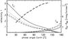 |
Fig. 1 Reflectivity of the Earth fE(αE,λ) and the Moon fM(αE,λ) for B (solid), V (dotted), R (dashed), and I (dash-dot). The thick dashed line is the difference of the surface brightness between earthshine Bes(αE,λ) and moonshine BM(αE,λ) for the 400−700 nm pass band. |
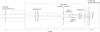 |
Fig. 2 Schematic overview of ESPOL with optical design and components drawn to scale. The focal mask is located in the focal plane of the 21 cm telescope. |
2. Instrumentation
2.1. Instrument requirements
The (surface) brightness of the lunar earthshine, the moonshine, and the contrast between the bright and dark sides of the Moon are described in the literature and summarized in Fig. 1. The reflectivity of the Moon fM(αM,λ) is from Kieffer & Stone (2005) and plotted as a function of the phase angle of the Earth αE using αE = 180° − αM. The reflectivity of the Earth fE(αE,λ) is from earthshine observations and model calculations by Pallé et al. (2003) for the pass band 400−700 nm. Due to the lack of multicolor earthshine observations the same shape for the reflectivity phase curve given by Pallé et al. (2003) is adopted for all colors and the curves for the different bands are just scaled with the factors derived from earthshine spectra from Arnold et al. (2002) as described in Sect. 7.4. Measurements of the surface brightness of the earthshine Bes(α,λ) and the moonshine BM(α,λ) were derived from observations of fiducial patches of highland regions (see also Qiu et al. 2003) by Montañés-Rodríguez et al. (2007) for the pass band 400−700 nm and Earth phase angles between αE = 30°−140°. In Fig. 1 we adopt their waxing Moon results and derive the mean daily surface brightness contrast Bes(λ) − BM(λ) between the dark and the bright side of the Moon. For α = 90° (half moon) the surface brightness of the earthshine is 14.9 mag/arcsec2. The difference between earthshine and moonshine ranges from 8−12 mag/arcsec2 between αE = 30°−140°.
The surface brightness of the earthshine is highest for the new moon phase and decreases with the Sun-Earth-Moon phase angle α (Fig. 1). Observations for small α near new moon require daytime or twilight observations for which a correction for the sky light is impossible or difficult. For α ≈ 45° an observational window of roughly 30 minutes with reasonably dark sky conditions becomes available after sunset or before sunrise for useful earthshine polarization measurements.
Observations during the night with much reduced sky background levels are possible for larger α, but the brightness of the moonshine due to the solar illumination increases rapidly (Fig. 1). At around α ≈ 90° the contrast between moonshine and earthshine becomes greater than about 104 and the light scattering in the Earth atmosphere and the instrument becomes more and more a problem for earthshine observations particularly in the red where the moonshine is strong and the earthshine weak. The light from the twilight sky and the moonshine are both strongly polarized p > 3%, and this needs to be considered for an accurate measurement of the earthshine polarization. The polarization of the moonshine is discussed in detail in Sect. 5.3.
2.2. The earthshine polarimeter
The EarthShine POLarimeter (ESPOL) measuring concept takes the background and stray light conditions for earthshine observations into account. The instrument allows imaging polarimetry of the entire Moon and the surrounding sky regions in order to measure the polarization signal of the weak earthshine on top of the strong stray light from the moonshine and/or the light contribution from the sky. ESPOL includes in addition exchangeable focal plane masks to block the light from the bright moonshine. The blocking of the bright crescent is required to allow for integrations of a few seconds without heavy detector saturation.
ESPOL is a dual-beam imaging linear polarimeter based on the rotating half-wave retarder plate and Wollaston polarization beam splitter concept. A schematic overview of the instrument is given in Fig. 2. The instrument includes a holder for exchangeable focal masks with different Moon-phase shapes to block the light from the bright lunar crescent in order to avoid heavy detector saturation. ESPOL uses a superachromatic λ/2 retarder plate on a motorized rotational stage for polarization beam switching and the selection of the Q and U polarization direction. The following Wollaston prism splits the light into the ordinary i∥ and extraordinary i⊥ beams with polarizations that are perpendicular to each other. Both beams, each with a field of view of 50′ × 40′, are imaged on the same 3072 × 2048 pixel CCD detector with a pixel scale of 1.5 arcsec/pixel. For our measurements we used a pixel binning of 3 × 3 pixels, which reduced the spatial resolution to roughly 10 arcsec.
Color or neutral density filters with a diameter of 5 cm or 2 inches can be inserted into the five-position filter wheel located in the collimated beam or into the camera filter wheel, respectively. To optimally align the focal masks to the orientation of the bright lunar crescent, the mask holder can be rotated around the optical axis. In addition the whole instrument can be rotated around the optical axis to fix the zeropoint of the polarization direction to any desired orientation.
ESPOL was built in-house for low costs using equipment for amateur astronomers and standard polarimetric and optical components for the wavelength range of 360−860 nm. The instrument is attached to an equatorially mounted 21 cm Dall-Kirkham Cassegrain telescope. A thermo-electrically cooled SBIG-STL 6303E camera with integrated filter wheel and shutter is used as the CCD system.
Figure 3 illustrates the data format delivered by the CCD. Because of the large field of view and the use of simple optical components, the system shows some image distortion in the north-south direction where the Moon diameter between ordinary and extraordinary beam differs by about 5%. These distortions can be tolerated because we are not interested in high spatial resolution but in the fractional polarization of extended surface regions.
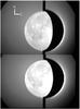 |
Fig. 3 ESPOL raw frame with the two polarization images i∥ and i⊥ of the earthshine on the Moon and the dark focal mask that blocks the light from the bright crescent. |
3. Observations
With ESPOL we measured the polarization of the earthshine for different phase angles and different wavelengths using a Bessell B,V,R,I filter set (Bessell & Murphy 2012). To minimize read-out overheads and detector noise the CCD was operated with 3 × 3 pixel binning providing a spatial resolution of about 10 arcsec, which is high enough for distinguishing mare and highland regions on the Moon. To minimize differential instrumental effects in the polarimetric signal the measurements have been performed in beam-exchange mode (Tinbergen 1996). Only the linear Stokes components Q/I and U/I are measured.
One polarimetric cycle consists of two measurements with half-wave plate positions 0° and 45° for Q/I and two measurements with positions 22.5° and − 22.5° for U/I. Typical integration times per exposure were about 2−10 s per half-wave plate position so that one full cycle could be recorded in about one minute. This is fast enough to avoid problems with guiding drifts and strongly changing atmospheric conditions. To improve the signal-to-noise ratio (S/N) a series of about five to ten such datasets were typically recorded for each wavelength band during one observing night.
ESPOL was rotated for all our measurements, including standard stars, into the orientation of the plane Sun-Earth-Moon so that the Stokes + Q direction is a polarization perpendicular to this plane and − Q a polarization in this plane. The Stokes ± U directions are ±45° with respect to this plane. The alignment was done by eye by rotating the complete instrument until the crescent shaped focal mask completely blocked the moonlight, which led to an alignment accuracy of about Δθ = ± 2°. For instrument monitoring and calibration, additional polarimetric measurements of the moonshine and polarized/unpolarized standard stars, as well as darks and twilight flatfield calibrations were recorded during each observing night.
Our data were collected during two observing runs in March and October 2011. For the run in March the instrument was installed at the former Swiss Federal Observatory in Zurich at an altitude of 470 m above sea level. This run served mainly for first instrument testing and data with limited wavelength and phase coverage were obtained. Despite the nonoptimal observing location in the heart of the city, the data quality was good enough to be included in this study. For the second run, we moved the instrument to the former Arosa Astrophysical Observatory at an altitude of 2050 m located in the Alps of eastern Switzerland. This site provides a much darker sky and a much reduced level of light scattering in the Earth atmosphere allowing measurements of the earthshine polarization for larger phase angles.
Both observing runs cover phase angles for the waxing Moon only. For the March measurements the earthshine originates mainly in the Atlantic Ocean, the Pacific Ocean, and the American continent, while in October the earthshine was due to reflected light from South America and the Atlantic Ocean. Table 1 gives an overview of the observed phase angles of our measurements, the used filters, and the number of polarization cycles for each filter.
Observing log.
4. Data reduction
4.1. Polarimetric reduction
Figure 3 shows a typical ESPOL raw frame with the ordinary i∥ and extraordinary i⊥ beams from the Wollaston showing the earthshine on the Moon in two opposite polarization directions. The bright crescent is blocked by the focal mask in order to suppress stray light in the instrument and to avoid disturbing detector saturation.
In the first data reduction step, the raw images were dark-subtracted before the two
opposite polarization images i∥ and
i⊥ for all half-wave plate orientations (0°,45°,22.5°, and
− 22.5°) were cut out and aligned. Then the fractional Stokes parameter
Q/I images were calculated according to the
beam-exchange method described in Tinbergen (1996):
 (3)where the first index of the image i
refers to the λ/2 retarder orientation, and ∥ and ⊥ indicate the
two opposite polarization states from the ordinary and extraordinary beams of the
Wollaston prism.
(3)where the first index of the image i
refers to the λ/2 retarder orientation, and ∥ and ⊥ indicate the
two opposite polarization states from the ordinary and extraordinary beams of the
Wollaston prism.
The corresponding intensity images are calculated by  (4)The polarization and intensity images for the
Stokes U measurements are determined in the same way but using the frames
taken with + 22.5° and − 22.5° retarder positions.
(4)The polarization and intensity images for the
Stokes U measurements are determined in the same way but using the frames
taken with + 22.5° and − 22.5° retarder positions.
In the differential polarization measurements, effects like the spatial variations of the system throughput, detector pixel-to-pixel sensitivity differences, and temporal changes between individual measurements are compensated to first order with the used double ratio, without any application of a flatfielding correction. Therefore, flatfielding was only applied on the intensity image IQ described in Eq. (4) using an intensity flatfield image produced in the same way.
As described above there are some image distortions due to the large field of view and the relatively simple optical setup. These differential distortions between the ordinary i∥ and extraordinary i⊥ beams disappear almost entirely in the double ratio method because images from both beams are in the nominator and denominator of that ratio. This first-order cancellation effect is not present in the summed intensity images and leads to some spatial smearing. Therefore the limb of the Moon is not sharp in the intensity image but on the more relevant larger scales, that is for identifying extended mare or highland regions, the image distortions are negligible. Nonetheless we have considered in our data analysis that small scale features may be affected by image distortion effects and the associated alignment inaccuracies.
The polarimetric properties of ESPOL were tested with observations of zero polarization standard stars β Tau, β UMa, γ Boo, (Turnshek et al. 1990), and Vega (Bhatt & Manoj 2000), which show that the instrumental polarization is ≤0.5% in all filters. From the polarized standard stars HD 21291, 9 Gem, φ Cas, 55 Cyg (Hsu & Breger 1982), we deduced a polarimetric efficiency above 98% and checked the zero point of the polarization direction.
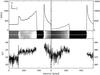 |
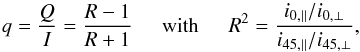
Fig. 4 Lunar west-east intensity (top) and polarization (bottom) profiles in the B band for phase 42.5° and 98.0° with a low (left) and high (right) stray light contribution from the moonshine, respectively. The panel in the middle shows the corresponding stripe of the intensity images. The profiles were extracted from 10 pixel wide regions as indicated by the dashed lines in the middle panel. |
4.2. Extracting the earthshine polarization
We are interested in the measurement of the fractional polarization of the earthshine
(Q/I)es, which needs to be extracted from
our data. Our observations show the contributions of three intensity components
 from the earthshine (es), the scattered light
from the moonshine (M), and the sky (see Fig. 4). In
our images it is rather easy to distinguish these components, assuming that the sky is
essentially constant over the whole field of view. The location of the earthshine is well
defined, and its intensity lies in a restricted range between the intensities of dark
maria and bright highlands. The scattered light intensity from the moonshine has a more
complex geometry. It is increasing rapidly toward the bright crescent, which is covered in
our data by the occulting mask.
from the earthshine (es), the scattered light
from the moonshine (M), and the sky (see Fig. 4). In
our images it is rather easy to distinguish these components, assuming that the sky is
essentially constant over the whole field of view. The location of the earthshine is well
defined, and its intensity lies in a restricted range between the intensities of dark
maria and bright highlands. The scattered light intensity from the moonshine has a more
complex geometry. It is increasing rapidly toward the bright crescent, which is covered in
our data by the occulting mask.
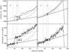 |
Fig. 5 Measuring the earthshine signals ΔI, ΔQ for relatively low (phase 73°, region #1, filter B) and high (phase 98°, region #1, filter R) moonshine levels with the background x′ and measuring regions x indicated. The dashed lines illustrate the guessed level of the background (mainly stray light) and background plus constant earthshine regions (reflected from maria). The full line is the linear extrapolation of the measured background from the x′ to the x region. |
The signatures of the three components can also be recognized in the fractional
polarization W-E cuts extracted from the Q/I images
shown in Fig. 4. The B-band
observation for phase 42.5° shows a significant sky contribution from the twilight. The
sky polarization is about 1.5% on the west side of the Moon, and the earthshine plus sky
polarization is about 3.5%. The polarization of the moonshine is slightly higher
(~4.5%) as can be seen near the east side of the occulting mask where the scattered
light of the moonshine dominates. For phase 98° the scattered moonshine dominates strongly
with a polarization of about 8%. The fractional polarization is just slightly enhanced at
the position of the earthshine. The (Q/I)-images consist
of the following contributions  (5)Because of our definition of the
± Q-directions perpendicular and parallel to the scattering plane, the
U/I polarization is essentially zero (≈±0.5%) and
dominated by noise.
(5)Because of our definition of the
± Q-directions perpendicular and parallel to the scattering plane, the
U/I polarization is essentially zero (≈±0.5%) and
dominated by noise.
Fractional polarization values (Q/I)es for the earthshine from the mare and highland regions of all our measurements and corresponding typical statistical 1σ uncertainties Δnoise.
After some investigation we defined a procedure for extracting the fractional earthshine
polarization (Q/I)es, which also provides
good results for large-phase angles, and the I filter for which the
signal is weak and/or the stray light from the moonshine is very strong. For small phase
angles, the earthshine signal is strong and the measurement is easy. The basic idea is to
measure the signal of the earthshine on top of the “background signal” in the
Itot frame and the Qtot frame
where
Qtot = (Q/I)tot Itot.
The “background signals” (bg) are just the sum of the contributions of the sky and the
moonshine
Ibg = Isky + IM
and
Qbg = Qsky + QM.
For this we extract radial cuts and extrapolate the background signal from the region
x′ outside to a location x inside the lunar disk
(Ibg(x′),
Qbg(x′) → Ibg(x),
Qbg(x)) where we measure the earthshine +
background level. The final signal is then
 (6)This procedure is illustrated in Fig. 5, for two cases. The first is a strong and clear
earthshine signal typical of phase angles α < 109° in the
B,V filters and phase angles α < 98° in the
R filter. The large majority of our data are of this kind. The other
case is typical of phase angles α ≥ 98° in the R and
I band filter for which the stray light from the moonshine dominates
strongly. The Q signal from the earthshine is still above but close to
the measuring limit. Also given are fits to the background, which in these cases mainly
consist of the moonshine plus a constant earthshine level fitted to the mare regions. The
use of a linear extrapolation of the background in the x′ region for the
background correction of the total earthshine plus background signal measured at
x seems reasonable (see also Qiu et al.
2003; Hamdani et al. 2006).
(6)This procedure is illustrated in Fig. 5, for two cases. The first is a strong and clear
earthshine signal typical of phase angles α < 109° in the
B,V filters and phase angles α < 98° in the
R filter. The large majority of our data are of this kind. The other
case is typical of phase angles α ≥ 98° in the R and
I band filter for which the stray light from the moonshine dominates
strongly. The Q signal from the earthshine is still above but close to
the measuring limit. Also given are fits to the background, which in these cases mainly
consist of the moonshine plus a constant earthshine level fitted to the mare regions. The
use of a linear extrapolation of the background in the x′ region for the
background correction of the total earthshine plus background signal measured at
x seems reasonable (see also Qiu et al.
2003; Hamdani et al. 2006).
We have investigated more complex background/straylight correction procedures, e.g. using three-parameter exponential fits, but they did not agree better than the linear extrapolation. Important for the accuracy of the earthshine measuring process is to select areas close to the western limb but not exactly at the limb because image alignment uncertainties of the polarimetric data reduction can create disturbing spurious features at the limb. The limb is also not a good measuring region because of the extreme incidence and reflection angles (near 90°) with respect to the large-scale surface normal that represents a situation that is not explored well for its backscattering properties.
All our data show that the differences between the lunar dark mare and bright highland regions are significant when determining the intensity and polarization of the backscattered earthshine. Therefore it is important to carry out separate measurements for these two main lunar surface types. Because of the strong albedo dependence (see Sect. 6), it is important that a chosen measurement field on the Moon does not have strong albedo variations. Under these terms we selected one mare field #1 in the Oceanus Procellarum area and one highland field #2 between Mare Humorum and the Moon’s limb as indicated in Fig. 6. Both fields are close to the western limb far away from the bright lunar side. They are available for measurements at all phase angles α when taking increasing stray light and the lunar libration into account. Therefore, for both fields a consistent data reduction could be carried out.
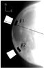 |
Fig. 6 Selected mare (#1) and highland (#2) fields used for the earthshine measurements, together with their background regions (white areas). |
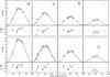 |
Fig. 7 Fractional polarization Q/I and U/I of the earthshine measured for highland (top) and mare regions (bottom) for the four different filters B,V,R, and I (left to right). The solid curves are qmaxsin2 fits to the data. The error bars give the statistical 1σ noise Δnoise of the data, whereas the mare I band data at phase angle 109.5° are additionally affected by a substantial systematic offset Δsyst > 0.5%. The dots in the V panel for the mare region indicate the measurements of Dollfus (1957) and a corresponding qmaxsin2 fit (dashed line) is also given. |
For both fields ten radial I and Q profiles separated by one degree were extracted, and ΔI and ΔQ were determined as described above. Table 2 gives the obtained (Q/I)es polarization values from both fields, which are also plotted in Fig. 7 as phase curves, together with the statistical 1σ error bars Δnoise.
As long as the S/N is sufficiently high, the linear extrapolation method is robust. The total uncertainty for the obtained fractional polarization of the earthshine for a highland or mare region at a particular date can be described by the statistical noise plus a predominantly positive systematic offset Δ(Q/I)es = Δsyst ± Δnoise.
The statistical 1σ uncertainty Δnoise is small (<0.3%). This follows from the scatter of the obtained values from different extraction cuts of the same day and includes random noise, but also hard to quantify systematic effects owing to small image drifts on the detector, changing stray light levels of the moonshine related to unstable atmospheric conditions, and perhaps other unidentified effects.
For observations with very small earthshine signals (i.e., at large phase angles and/or strong stray light of the moonshine), the linear extrapolation of the background introduces a systematic overestimate Δsyst of the result. This is because the moonshine-dominated stray light background increases with an upward curvature toward the illuminated crescent. For the B,V, and R measurements at phase angles <100° this offset is negligible or small (<0.5%); however, in the I band filter at phase angle 109.5° the systematic offset clearly dominates and the mare I band result for 109.5° is no longer useful (see Fig. 7). For this reason we disregard the mare I band result at 109.5°.
5. Earthshine polarization results
5.1. Data
The results for the fractional earthshine polarization Q/I measured in the Bessell B,V,R, and I bands are presented in Table 2 and Fig. 7. The plots in Fig. 7 also include the U/I data points and the estimated statistical 1σ uncertainties of the individual data points Δnoise. The mare V band panel also shows the measurements by Dollfus (1957), which are in good agreement with our data.
Our earthshine data show a tight correlation between the polarization taken simultaneously for the highland and mare regions. Independent of color filter and phase angle, the polarization for the mare region is a factor of 1.30 ± 0.01 higher than for the highland region as illustrated in Fig. 8.
Tight correlations are also found between different colors taken for the same observing date. When we plot the polarization (Q/I)es in the V,R, and I bands versus the polarization in the B band (Fig. 9), we find that the ratios are independent of αE. We get 0.72 ± 0.02, 0.49 ± 0.02, and 0.28 ± 0.05 for the ratios of the polarization between the V and B bands, R and B bands, and I and B bands respectively. Therefore, we conclude that to first order we can assume the same shape for the polarization phase curve for all wavelengths.
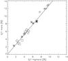 |
Fig. 8 Correlation between the fractional polarization for mare and highland regions measured simultaneously. The different symbols indicate the colors B(+), V(∗), R(⋄), and I(□). The line shows the derived proportionality factor 1.30 ± 0.01. |
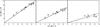 |
Fig. 9 Fractional polarization of the earthshine reflected at highland (+) and mare (∗) regions in V,R, and I bands (left to right) with respect to the B band. The lines indicate linear fits both for highland (solid) and mare (dashed) data separately. |
5.2. Fits for the phase dependence
The phase dependence of the earthshine polarization looks symmetric and can be well fitted with a simple qmaxsin2(α) curve. The model simulations by Stam (2008) for Earth-like planets also support phase curves qmaxsinp(α). She calculates polarization phase curves assuming a range of surface types (e.g., forest-covered areas with Lambertian reflection or dark ocean with specular reflection) and cloud coverages. We find that the broad shape of her model phase curves can be well fitted by curves ~qmaxsinp(α + α0) with p ≈ 1.5−3 and α0 ≈ 0°−10°.
Furthermore, she finds characteristic features at low phase angles owing to the rainbow effect and negative polarization at large phase angles caused by second-order scattering. We cannot assess the presence of such features because of the coarse phase sampling of our data.
Besides the qmaxsin2(α) curve we also tried functions with more free parameters to fit the data, such as using a curve like qmaxsinp(α + α0), varying the exponent p between values of 1.5−3 and by introducing a phase shift α0. However, such fits do not provide a significantly better match to the data. Because our data predominantly cover phase angles around quadrature the shape of the phase curve is not very well constrained.
The derived qmax fit parameters for the different phase
curves are given in Table 2, along with the
standard deviation of the data points from the fit σd−f. For
Q/I the typical σd−f is
≈0.2% in good agreement with the typical 1σ uncertainty of the individual
data points Δnoise. The standard deviation of the derived
U/I values from the expected zero-value is only
slightly higher and typically ≈0.3%, indicating that the instrument alignment with respect
to the Sun-Earth-Moon plane was excellent (see Sect. 3). The U signal is at the level of the measurement noise
| U| ≈ Δnoise(U). Therefore one should not
use the normalized total polarization  because the square in this formula
introduces systematic errors. However, we estimate that the impact of
U/I to the total polarization p is less than ±0.05%.
Therefore we use p ≅ Q/I and neglect
the U component in the subsequent discussion.
because the square in this formula
introduces systematic errors. However, we estimate that the impact of
U/I to the total polarization p is less than ±0.05%.
Therefore we use p ≅ Q/I and neglect
the U component in the subsequent discussion.
5.3. The moonshine polarization
As a check of our polarimetry we can compare the polarization of the stray light from the moonshine with values from Coyne & Pellicori (1970) and Dollfus & Bowell (1971). Forward scattering in the Earth atmosphere with scattering angles less than a few degrees does not introduce a significant polarization effect. Therefore, we can assume that the polarization of the lunar stray light (Q/I)M represents the polarization of the bright lunar crescent well. For areas just east of the Moon close to the focal mask (see Fig. 4) the scattered moonshine dominates strongly. There we can neglect the contribution of the sky background (Q/I)sky and assume that (Q/I)bg ≈ (Q/I)M.
Figure 10 compares our results with the waxing Moon values given by Coyne & Pellicori (1970). They used different filters but their B′ and Gm bands (λeff [μm] = 0.45, 0.53) are close to our B and V bands, and the good agreement with our data underlines the consistency of our polarimetric data reduction.
Unfortunately, Coyne & Pellicori (1970) used no
red filters, but the scaled Gm phase curve fits our
R and I band data also well if scaling parameters of
0.80 and 0.65 are used. This is in good agreement with the wavelength dependency of the
maximum degree of polarization Pmax of the whole Moon
presented in Dollfus & Bowell (1971):
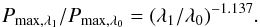 (7)With this formula we obtain color ratios of
q(R)/q(Gm) = 0.81
and
q(I)/q(Gm) = 0.64
for the Moon polarization in good agreement with the above scaling parameters derived from
our stray light data.
(7)With this formula we obtain color ratios of
q(R)/q(Gm) = 0.81
and
q(I)/q(Gm) = 0.64
for the Moon polarization in good agreement with the above scaling parameters derived from
our stray light data.
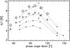 |
Fig. 10 Measured polarization of the lunar stray light near the focal mask in the B,V,R, and I filters (from top to bottom by filled dots and dashed lines). Also indicated are the polarization values given by Coyne & Pellicori (1970) for the disk integrated moonshine of the waxing Moon in their B′ (⋄) and Gm bands (+). |
6. A correction for the depolarization due to backscattering at the lunar surface
The polarized light from the Earth is depolarized by the backscattering at the particulate
surface of the Moon. We express this effect as polarization efficiency ϵ,
to describe the fraction of linear polarization preserved. We simplify the treatment by only
considering the Q linear polarization direction perpendicular and parallel
to the scattering plane Sun-Earth-Moon. Then the polarization efficiency is
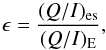 where
(Q/I)E is the Earth polarization. The
polarization efficiency
ϵ(λ,aλ)
depends on the wavelength and the surface albedo. We neglect the phase dependence because
the scattering angle is always 179° ± 0.5°.
where
(Q/I)E is the Earth polarization. The
polarization efficiency
ϵ(λ,aλ)
depends on the wavelength and the surface albedo. We neglect the phase dependence because
the scattering angle is always 179° ± 0.5°.
The depolarization of the lunar surface has already been investigated by Lyot (1929) and Dollfus (1957). They measured the depolarization due to backscattering at volcanic ashes and fines, which were used as proxies for the lunar soil. They found a well-defined anticorrelation between albedo and polarimetric efficiency.
Most important for determining ϵ(λ,a) are the albedo and polarization measurements for the reflection from several Apollo lunar soil samples by Hapke et al. (1993, 1998). They illuminated eight samples under an inclination of five degrees (to avoid specular reflection) with 100% polarized blue and red light and measured the ratio of I⊥/I∥ for phase angles 1° (~backscattering) to 19° or scattering angles of 179° to 161°. The results for the linear polarization ratio are presented in Hapke et al. (1993) in graphical form, and we extracted the data for phase angle 1° and derived the polarization efficiency ϵ. The normal albedos are only given for a phase angle of 5° (Hapke et al. 1993, Table 1), and we converted them into earthshine backscatter albedos corresponding to 1° phase angle by applying a conversion factor of 1.25 ± 0.05. We derived this factor from albedo phase curves presented in Velikodsky et al. (2011) where they give a comprehensive summary of the results of various independent photometric observations of the Moon including their own, Clementine data, and ROLO data.
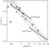 |
Fig. 11 Linear polarization efficiency as function of the normal albedo at 1° (Eq. (9)) for the B (dashed), V (dash-dot), R (solid), and I (dash-dot-dot) band. More information about the fit procedure to the Hapke et al. (1993) samples in the red (⋄) and the blue (+) is given in the text. Measurements of the same sample are connected by dotted lines. The thick black lines show the derived wavelength and albedo-dependent polarization efficiencies for our two measurement areas #1 and #2 (Fig. 6). |
The samples from Hapke et al. (1993) include five low albedo samples ared ≈ 0.09−0.13 representative of maria, two higher albedo samples ared ≈ 0.15−0.19 representative of highlands, and one atypical, extremly high albedo sample with normal albedo ared > 0.35. This sample with NASA number 61221 was taken from white material at the bottom of a trench (see The Lunar Sample Compendium1), and we therefore treat this sample as special case in our analysis.
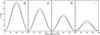 |
Fig. 12 Depolarization-corrected polarization phase curves of Earth in the B,V,R, and I bands. The solid line indicates the mean of the mare (dashed) and highland (dash-dot) results based on the polarization efficiency correction derived in this work. |
Figure 11 shows the polarization efficiencies for the measurements of Hapke et al. (1993) as a function of the 1°-albedo for a blue wavelength (λ = 442 nm) and a red wavelength (λ = 633 nm). The figure nicely illustrates the clear anticorrelation between albedo a and polarization efficiency ϵ.
We consider now the backscatter properties of the lunar samples in more detail. All
samples, except 61221, show a very similar color dependence in their albedo with
ared/ablue = 1.35
(σ = 0.05). This agrees with the spectral variation of the mean lunar
albedo  from Dollfus & Bowell (1971) (see also Gehrels et al. 1964, Table XIII; and Velikodsky et al. 2011, Table 2) described by
![Mathematical equation: \begin{equation} \label{albedo dependence} {\rm log}\, \bar{a} = 0.83 \, {\rm log}\, \lambda [\mu{\rm m}] - 0.80. \end{equation}](/articles/aa/full_html/2013/08/aa21855-13/aa21855-13-eq214.png) (8)Inserting the wavelengths of the Hapke et al. (1993) measurements into this formula yields
(8)Inserting the wavelengths of the Hapke et al. (1993) measurements into this formula yields
 ,
in very good agreement with the albedo ratio derived above for the lunar samples.
,
in very good agreement with the albedo ratio derived above for the lunar samples.
For most samples the polarization efficiency is slightly higher (in one case equal) in the blue than in the red. There is one notable exception, which is sample number 79221. Although the albedo of sample 79221 is lower in the blue than in the red, its polarization efficiency is not higher in the blue as is the case in all other samples. Also when looking into reflectivity studies for this sample (e.g. Noble et al. 2001), it is not clear why this sample could behave differently in its depolarization properties than other maria soils. Therefore, we treat sample 79221 as an exception.
If we disregard sample 79221, then the remaining six samples have an average color dependence for their polarization efficiency ratio of ϵred/ϵblue = 0.91 (σ = 0.05). Including sample 79 221 gives a mean ratio of 0.96 but a standard deviation that is significantly higher with 0.14.
Based on these backscatter measurements of lunar samples, we derived a two-dimensional
linear fit for the polarization efficiency log ϵ as function of
log a603, the albedo at 603 nm, and log λ
for the wavelength ![Mathematical equation: \begin{equation} \label{eq:pvsa} {\rm log}\, \epsilon(\lambda, a_{603}) = -0.61 \,{\rm log}\, a_{603} - 0.291 \, {\rm log}\, \lambda \,[\mu{\rm m}] - 0.955 . \end{equation}](/articles/aa/full_html/2013/08/aa21855-13/aa21855-13-eq221.png) (9)For this fit the wavelength dependence of the
albedo has been assumed to follow Eq. (8),
and it was normalized to 603 nm. By fitting the red data points, we find the logarithmic
slope − 0.61 ± 0.04 between the polarization efficiency ϵ and the albedo
ared, which we also adopted for the blue data points. Finally,
by fitting over the red and blue points separately, we determined the other two parameters
− 0.291 and − 0.955. The resulting relation for the linear polarization efficiency as a
function of the normal albedo at 1° is shown in Fig. 11 for the B,V,R, and I bands.
(9)For this fit the wavelength dependence of the
albedo has been assumed to follow Eq. (8),
and it was normalized to 603 nm. By fitting the red data points, we find the logarithmic
slope − 0.61 ± 0.04 between the polarization efficiency ϵ and the albedo
ared, which we also adopted for the blue data points. Finally,
by fitting over the red and blue points separately, we determined the other two parameters
− 0.291 and − 0.955. The resulting relation for the linear polarization efficiency as a
function of the normal albedo at 1° is shown in Fig. 11 for the B,V,R, and I bands.
For deriving the albedos of our measurement regions we used the results of Velikodsky et al. (2011), who present maps of lunar apparent and equigonal albedos at phase angles 1.7°−73° at wavelength 603 nm. We extrapolated their results to a phase angle of 1° and get albedos a#1(603 nm) = 0.11 ± 0.01 and a#2(603 nm) = 0.21 ± 0.01. The resulting polarization efficiencies ϵ#1(λ,a603) and ϵ#2(λ,a603) are listed in Table 2 for the B,V,R, and I bands and shown in Fig. 11 giving the ϵ(λ,a603) fits. Overall we estimate the uncertainty of the derived polarization efficiency to be Δϵ ≈ ± 3%.
The main uncertainty of this derivation stems from the uncertainty in the above-mentioned albedo conversion from α = 5° into albedos corresponding to 1° phase angle where the conversion factor 1.25 ± 0.05 leads to an uncertainty of the polarization efficiency of about Δϵ = ± 1.5%. To significantly improve the determination of ϵ accurate lunar albedo maps for backscatter geometry are required. This is because backscattering by ≈1°, is strongly influenced by the opposition effect of the lunar surface, that is a steep brightness surge which comes from coherent backscattering and shadow hiding (e.g. Shkuratov et al. 2011, and references therein). In addition to that, the Hapke et al. (1993, 1998) sample might not be representative of the surface properties of the Moon.
The logarithmic slope − 0.61 ± 0.04 is better constrained for the low-albedo samples, and it introduces an uncertainty Δϵ = ± 1% toward the higher albedo samples. Moreover, the logarithmic relation might not be valid over the complete albedo range between aλ = 0.09−0.19, so two slopes, one for the maria and one for the highlands, might be necessary. However, based on the available samples, this is not obvious, and one log fit may not be the best representation of the data. More direct measurements of the polarization efficiency of lunar backscattering are required to reduce this source of uncertainty.
7. Polarization of planet Earth
7.1. Fractional polarization derived from the earthshine
In Fig. 12 we present the depolarization-corrected polarization phase curves of planet Earth in the B,V,R, and I bands, and the corresponding corrected fit parameters qmax,corr are listed in Table 2. For the B band we obtain a maximum polarization of about 25% that decreases with wavelength to about 8% in the I band. For perfect measurements and perfect polarization efficiency corrections, the same Earth polarization qmax,corr values should be obtained for the mare and highland regions. We note that the corrected highland results are systematically higher than the mare results by a factor of about 1.1 for the B,V,R bands and 1.4 for the I band. This also reflects the uncertainty in our determination of the polarization efficiency of backscattering at the Moon Δϵ ≈ ± 3% derived in Sect. 6.
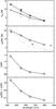 |
Fig. 13 Top: Earthshine polarization results at quadrature for maria (∗) and highlands (+). The thin lines give the Sterzik et al. (2012) spectro-polarimetry for waning (dashed) and waxing (dotted) moon at Earth phases 87° and 102°, respectively, and the Takahashi et al. (2013) spectro-polarimetry (dash-dot) at 96°. The circles are the Dollfus (1957) values qmax from Fig. 7 (filled) and two additional observations at Earth phase ≈ 100° (open). 2nd panel: Earth polarization pE from Table 3 (⋄) compared to the POLDER/ADEOS results of Wolstencroft & Breon (2005) (×) and two Stam (2008) models with 40% (dash-dot) and 60% (dash-dot-dot) cloud coverage. Bottom two panels: spectral reflectivity of Earth fE and polarized reflectivity of Earth pE × fE. |
7.2. Comparison with previous measurements
In Fig. 7 we compare our earthshine measurements with the pioneering study of Dollfus (1957), who obtained his data with visual observations using a “fringed-field polariscope”. The agreement with our V band phase curve for the mare region is excellent. If we apply qmaxsin2 fits (see Sect. 5.2) to both data sets, the quadrature signals only differ by 0.8%. The small deviations between Dollfus (1957) and us can be explained by different mare regions that were observed and the expectedly non-equal effective wavelengths of the two completely different types of measurements. For one night at α ≈ 100°, Dollfus (1957) also reports the earthshine polarization in two filters, namely p = 5.4% for 0.55 μm (V′ band) and 3.5% for 0.63 μm (R′ band). The ratio pV′/pR′ = 1.54 is again in good agreement with our polarization ratio qmax,V/qmax,R = 1.47. This indicates that the filters used by Dollfus (1957) must match our filter pass bands quite well.
The spectral dependence of the earthshine polarization observed with a spectral resolution of 3 nm was recently published by Sterzik et al. (2012). These sensitive spectro-polarimetric data reveal weak, narrow features of the Earth due to O2 and H2O on a smooth polarization spectrum decreasing steadily from the blue toward longer wavelengths. They present measurements for two epochs with phase angles α = 87° for a waning moon phase and α = 102° for a waxing moon phase. For the waning moon case they obtained an earthshine polarization of about pB = 12.1% in the B band, pV = 7.7% in V, pR = 5.6% in R, pI = 3.9% in I, and a significantly higher polarization for the waxing moon phase with pB = 16.6%, pV = 9.7%, pR = 8.0%, and pI = 6.7%, as plotted in Fig. 13. Unfortunately, it is not clear whether they measured the backscattering from maria or highlands. Sterzik et al. (2012) attribute the polarization differences between the two epochs mainly to intrinsic differences in the polarization of Earth because the earthshine stems from different surface areas and were taken for days with different cloud coverage. Considering our polarization values for highlands and maria, then it could be possible that the differences measured by Sterzik et al. (2012) are at least partly due to the mare/highland depolarization difference (or surface albedo difference).
Another spectra-polarimetric observation of the earthshine was published by Takahashi et al. (2013). They also find a rise in the fractional polarization of the earthshine toward the blue but with a much flatter slope. Unfortunately, they do not report whether their results were obtained from maria or highlands either. Therefore, only a qualitative comparison with our data can be made. The observations of Takahashi et al. (2013) are conducted on five consecutive nights and cover phase angles α = 49°−96°. In the blue they find that the maximum polarization is reached at α ≈ 90°. However, for wavelengths >600 nm, the polarization keeps increasing up to and including their last measurement at α = 96°. They conclude that the phase with the highest fractional polarization αmax is shifted toward larger phase angles, which could be explained by an increasing contribution of the Earth surface reflection. In our data we do not see this shift, but neither can we exclude it because we were not able to derive meaningful data due to the very strong stray light from the moonshine and the weak signal from the earthshine. In this regime our linear extrapolation method of subtracting the background stray light from the earthshine signal introduces a strong systematic overestimate Δsyst of the result (see Sect. 4.2). Takahashi et al. (2013) also use a linear extrapolation method to determine the earthshine polarization, but unfortunately they do not describe their data reduction in detail. Therefore, considering the limitations of our linear extrapolation, it could be possible that the shift of αmax reported by Takahashi et al. (2013) is due to the strong stray light at phase angles >90°.
Overall, the spectral dependence of the polarization of Sterzik et al. (2012) and Takahashi et al. (2013) is qualitatively similar to our measurements, but the level and slope of the fractional polarization differ quantitatively. Because Sterzik et al. (2012) and Takahashi et al. (2013) provide no information about the lunar surface albedo for their measuring area and do not assess the stray light effects from the bright moonshine, their results cannot be used for a quantitative test of our results. The spectral slope of Sterzik et al. (2012) is slightly steeper than ours, while the slope of Takahashi et al. (2013) is slightly flatter.
For an assessment of the polarization efficiency for the lunar backscattering we used literature data for polarimetric measurements of lunar samples by Hapke et al. (1993, 1998) and derived a wavelength and surface-albedo dependent polarization efficiency relation ϵ(λ,a603), which gives ϵ(V,0.11) = 50.8% for mare in the V band. This value is significantly higher than the 33% derived by Dollfus (1957), which he based on the analysis of volcanic samples from Earth used as a proxy for the lunar maria. Because of this, the Earth polarization derived in this work is much lower than the value given in Dollfus (1957). We are not aware of other studies of the polarization efficiency ϵ for the lunar backscattering. Relying on the determination of ϵ on real lunar soil is certainly an important step in the right direction for a more accurate determination of the polarization of Earth.
Very valuable are the reported Earth polarization values from Wolstencroft & Breon (2005) based on direct polarization measurements with the POLDER instrument on the ADEOS satellite. They derived the fractional polarization for the wavelengths 443 nm (B′), 670 nm (R′), and 865 nm (I′) for different surface types and cloud coverage. Weighted mean values representative of an integrated planet Earth observation (55% cloud coverage) of 22.6%, 8.6%, and 7.3% in the B′,R′, and I′ bands are obtained, which are also indicated in the second panel of Fig. 13. The good agreement between our derivation based on the earthshine and the values from Wolstencroft & Breon (2005) confirms our determination of the polarization efficiency. Unfortunately, it is not possible to assess whether the R band point of this study differs significantly from the value of Wolstencroft & Breon (2005) because they give no description of their data and uncertainties.
7.3. Comparison with the models from Stam (2008)
The study of Stam (2008) is unique for modeling the spectral dependence of the fractional polarization of Earth-like planets. In her work she also explored dependencies on a range of physical properties different from Earth’s. For our comparison we pick the model for an inhomogeneous Earth-like planet with 70% of the surface covered by a specular reflecting ocean and 30% by deciduous forest (Lambertian reflector with an albedo for forest), and cloud coverages 40% and 60%. When compared to our Earth polarization determinations (Fig. 13, second panel), these models agree with our measurements at short wavelengths but show a clear deficit in the fractional polarization at long wavelengths in the I band. This is not surprising since the models were not tuned to the case of Earth. In the models, only very thick, liquid water clouds were included, but no thin liquid water clouds and no ice clouds. Karalidi et al. (2012) shows that with more realistic cloud properties for Earth, the degree of polarization can vary strongly depending on the cloud’s optical thickness. Our data could now be used to test and to improve model calculations for the Earth polarization.
7.4. Polarization flux contrast for the Earth – Sun system
A key parameter for the polarimetric search and characterization of Earth-like extrasolar planets is the polarization flux p × f of a planet or the polarization flux contrast Cp as described in Eq. (2). The polarization flux of a highly polarized planet is easier to measure than the fractional polarization p, because the reflected intensity cannot be distinguished easily from the scattered light halo of the central star in high contrast observations. But because stars are essentially unpolarized, it should be possible to detect a differential signal of polarized light from extrasolar planets with high contrast polarimetric imagers as foreseen for the upcoming instrument SPHERE/VLT and planned for future facilities like the E-ELT (e.g. Schmid et al. 2006; Beuzit et al. 2008; Kasper et al. 2010). The polarimetric detection of an Earth-like planet is difficult; nonetheless, it is useful to have accurate values for the expected signal to plan such observations.
The prediction of the polarization flux of an exo-Earth requires besides the fractional
polarization p(α,λ) determined in this work also the
reflected intensity f(α,λ). The reflected intensity of
Earth can be split into a wavelength dependent geometric albedo term
Ag(λ) = f(0°,λ)
and a normalized phase dependence Φ(α)/Φ0 where
Φ0 = Φ(α = 0) according to
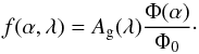 With this approach we neglect the color
dependence of the phase curve, which is not known but certainly small when compared to the
measuring uncertainties for the spectral albedo
Ag(λ) and the uncertainties in the
fractional polarization pE(λ,α).
With this approach we neglect the color
dependence of the phase curve, which is not known but certainly small when compared to the
measuring uncertainties for the spectral albedo
Ag(λ) and the uncertainties in the
fractional polarization pE(λ,α).
The visual geometric albedo of Earth is Ag(V) = 0.367 (Cox 2000). With the relative spectral reflectance measured by Arnold et al. (2002), Woolf et al. (2002), and Montañés-Rodriguez et al. (2005), we deduce the geometric albedo for the individual B,V,R, and I filters as given in Table 3.
For the phase dependence Φ(α)/Φ0 we use the phase curve determined by Pallé et al. (2003) for the 400−700 nm filter normalized to the B,V,R, and I band geometric albedos derived above. The derived phase curves are given in Fig. 1, and their value for Φ(90°)/Φ0 = 0.27 yields the polarized reflectivity for quadrature phase pE(90) × fE(90) for the B,V,R, and I filters as plotted in Fig. 13 and given in Table 3.
The phase curve  of Pallé et al. (2003) is based on earthshine
measurements at phases between α = 30°−145° extrapolated to
α = 0°−180°. This broad phase angle coverage is unique and remains, to
our knowledge, the only available observation of the phase dependence
Φ(α) of fE. For future reference we also give
in Table 3 the phase integral parameter
As/Ag, the ratio between
spherical and geometric albedo, derived from the Pallé
et al. (2003) data.
of Pallé et al. (2003) is based on earthshine
measurements at phases between α = 30°−145° extrapolated to
α = 0°−180°. This broad phase angle coverage is unique and remains, to
our knowledge, the only available observation of the phase dependence
Φ(α) of fE. For future reference we also give
in Table 3 the phase integral parameter
As/Ag, the ratio between
spherical and geometric albedo, derived from the Pallé
et al. (2003) data.
The spectral dependence of the polarization flux pE(λ,90°) × fE(λ,90°) of Earth decreases steeply toward longer wavelengths, because both the fractional polarization pE and the reflectivity fE are higher for the blue than for the red. The pE × fE signal in the B band is about a factor five times stronger than in the I band.
The polarization contrast Cp(λ,90°)
according to Eq. (2) is determined from
pE × fE and using
 . This yields values at the level of a few
times 10-11 only (Table 3). One should
note that an Earth-like planet in the habitable zone of an ≈M4V star with
L = 0.02 L⊙ is at a much smaller
separation of 0.14 AU. In this case the expected polarization contrast is about a factor
of 50 higher and within reach for a high contrast imaging polarimeter at an ELT (Kasper et
al. 2010).
. This yields values at the level of a few
times 10-11 only (Table 3). One should
note that an Earth-like planet in the habitable zone of an ≈M4V star with
L = 0.02 L⊙ is at a much smaller
separation of 0.14 AU. In this case the expected polarization contrast is about a factor
of 50 higher and within reach for a high contrast imaging polarimeter at an ELT (Kasper et
al. 2010).
The B,V,R, and I phase curves for the polarized reflectivity pE × fE are plotted in Fig. 14. The maximum signal occurs near α ≈ 65°, which is thus the best phase for a detection.
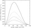 |
Fig. 14 Polarized reflectivity phase curve pE(α) × fE(α) for Earth in the B (solid), V (dotted), R (dashed), and I band (dash-dot). |
Geometric albedo Ag, phase integral As/Ag, and quadrature results for the planet Earth.
8. Summary and discussion
This work presented measurements of the earthshine polarization in the B,V,R, and I bands. The data were acquired with a specially designed, wide-field imaging polarimeter using a focal plane mask to suppress the light from the bright lunar crescent. Thanks to this measuring method we could accurately correct for contributions from the (twilight) sky and the scattered light from the bright lunar crescent and derive values with well-understood uncertainties. We derived phase curves for the fractional polarization for the earthshine reflected from maria and highlands for the different filter bands. The phase curves can be fit with the sine-square function qmaxsin2(α). The amplitude qmax decreases strongly with wavelength from about 13% in the B band to about 3% in the I band (see Table 2). The fractional polarization of the earthshine is about a factor 1.3 higher for the dark mare region when compared to the bright highland. Our phase curve for the mare region in the V band is in close agreement with the historic visual polarization phase curve from Dollfus (1957).
We studied the depolarization introduced by backscattering at the lunar surface based on published polarimetric measurements of lunar samples (Hapke et al. 1993, 1998). We derived a two-dimensional fit function for the polarization efficiency ϵ(λ,a603) of the backscattering, which depends on wavelength and surface albedo. Earthshine measurements plus ϵ correction yield as the main result of this paper the fractional polarization of the reflected light from the planet Earth as a function of phase in four bands. The polarization of Earth in quadrature phase is as high as 25% in the B band and decreases steadily with wavelength to 8% in the I band (see Table 3). Similar values have been reported from direct satellite measurements of the Earth polarization (Wolstencroft & Breon 2005).
This work provides the most comprehensive measurements of the polarization of the integrated light of the planet Earth up to now. The determined values can be used as benchmark values for tests of polarization models and for predictions for future polarimetric observations of Earth-like extrasolar planets. In particular, we accurately described our measurements and assessed the uncertainties. In addition we applied a polarization efficiency ϵ correction. For the first time, it is based on lunar soil measurements and is significantly different from previously used volcanic rock measurements.
Similar to our data of Earth, the models of Stam (2008) for horizontally inhomogeneous Earth-like planets with thick liquid water cloud coverage show also a decrease in fractional polarization with wavelength but with a significantly steeper slope. This may indicate that other scattering components, for example aerosols, thin liquid water clouds, and ice clouds contribute significantly to the Earth polarization in the I band (see Karalidi et al. 2012).
Are our polarization values for the planet Earth representative or should we expect large temporal variations? Our data were taken during two observing runs each lasting a few days. Two data sets are from similar phase angles, 73.0° and 75.5°, but they were taken seven months apart. The measured fractional polarization differs by about Δq/q ≈ 0.1. Also the deviation of the data points from the fit qfit = qmaxsin2α is at the same level (| q − qfit|)/q ≈ 0.1. This scatter is at the level of our calibration errors. Therefore, variation in the intrinsic polarization signal of Earth on the 10% level could be present in our data without being recognized. Our measurements certainly show no changes at the Δq/q ≈ 0.3 level as suggested by Sterzik et al. (2012). Variations in the fractional polarization are of interest because they could be used as a diagnostic tool for investigations of surface structures or temporal changes in the cloud coverage of extrasolar planets.
Because our study includes a detailed assessment of the uncertainties for each step in our determination, we can now discuss how the Earth polarization measurement could be improved. Polarization variability studies could be carried out with enhanced sensitivity by selecting observing periods and filters with strong earthshine polarization signals in order to minimize statistical noise and systematic effects in the data extraction. Observations in the B and V filter, and for phase angles in the range from α = 40° to 100°, would be ideal for such studies. Measurements taken for several consecutive nights would allow a sensitive search for day-to-day variations at a level of Δq/q ≈ 0.03 owing to variable cloud coverage. Also multiple-epoch data could be collected for an investigation of long-term and seasonal polarization changes.
The determination of a more accurate wavelength dependence of the earthshine polarization could be established with long integrations for phase angles between 50°−80° when the earthshine polarization signal is strong, the level of scattered light from the moonshine still low, and the time for observations after twilight long enough for observations in multiple filters.
More accurate phase curves require careful analysis of the data from different phases because the earthshine observing conditions and the associated measuring and calibration procedures change strongly with lunar phase. If these problems can be solved, then one could accurately determine the peak in the fractional polarization curve near α = 90° as function of wavelength and investigate the presence of a rainbow feature in the polarization data around α = 40° (see Stam 2008).
A more accurate absolute value for the polarization of the planet Earth first requires more data to average out intrinsic variations. Equally important is a more accurate determination of the surface albedo for the measuring region and the associated polarization efficiency ϵ(λ,aλ) for the correction of the lunar backscattering.
The imaging polarimetry of the earthshine presented in this study and the spectro-polarimetric results from Sterzik et al. (2012) and Takahashi et al. (2013) demonstrate that investigating the Earth polarization via earthshine measurements is very useful and attractive. Detailed and versatile investigations are possible with existing polarimetric instruments as used by Sterzik et al. (2012) and Takahashi et al. (2013) or with small, specific experiments as demonstrated in this work. The obtained results can be compared with model calculations like those described in Stam (2008) and teach us about the light-scattering processes of planets. Because we know our Earth so well, we can also investigate subtle effects, which are potentially important in other planets. Building up our knowledge of scattering polarization from Earth could therefore become important for the future polarimetric investigation of extrasolar planets.
Acknowledgments
Part of this work was supported by the FINES research fund by a grant through the Swiss National Science Foundation (SNF).
References
- Arnold, L., Gillet, S., Lardière, O., Riaud, P., & Schneider, J. 2002, A&A, 392, 231 [NASA ADS] [CrossRef] [EDP Sciences] [MathSciNet] [Google Scholar]
- Bailey, J. 2007, Astrobiology, 7, 320 [NASA ADS] [CrossRef] [PubMed] [Google Scholar]
- Bessell, M., & Murphy, S. 2012, PASP, 124, 140 [Google Scholar]
- Beuzit, J.-L., Feldt, M., Dohlen, K., et al. 2008, in SPIE Conf. Ser., 7014 [Google Scholar]
- Bhatt, H. C., & Manoj, P. 2000, A&A, 362, 978 [NASA ADS] [Google Scholar]
- Cox, A. N. 2000, Allen’s astrophysical quantities (New York: AIP Press: Springer) [Google Scholar]
- Coyne, G. V., & Pellicori, S. F. 1970, AJ, 75, 54 [NASA ADS] [CrossRef] [Google Scholar]
- Dollfus, A. 1957, Supplements aux Annales d’Astrophysique, 4, 3 [Google Scholar]
- Dollfus, A., & Bowell, E. 1971, A&A, 10, 29 [NASA ADS] [Google Scholar]
- Dumusque, X., Pepe, F., Lovis, C., et al. 2012, Nature, 491, 207 [NASA ADS] [CrossRef] [PubMed] [Google Scholar]
- Gehrels, T., Coffeen, T., & Owings, D. 1964, AJ, 69, 826 [NASA ADS] [CrossRef] [Google Scholar]
- Hamdani, S., Arnold, L., Foellmi, C., et al. 2006, A&A, 460, 617 [NASA ADS] [CrossRef] [EDP Sciences] [Google Scholar]
- Hapke, B. W., Nelson, R. M., & Smythe, W. D. 1993, Science, 260, 509 [NASA ADS] [CrossRef] [PubMed] [Google Scholar]
- Hapke, B., Nelson, R., & Smythe, W. 1998, Icarus, 133, 89 [NASA ADS] [CrossRef] [Google Scholar]
- Howard, A. W., Marcy, G. W., Bryson, S. T., et al. 2012, ApJS, 201, 15 [NASA ADS] [CrossRef] [Google Scholar]
- Hsu, J.-C., & Breger, M. 1982, ApJ, 262, 732 [NASA ADS] [CrossRef] [Google Scholar]
- Karalidi, T., Stam, D. M., & Hovenier, J. W. 2011, A&A, 530, A69 [NASA ADS] [CrossRef] [EDP Sciences] [Google Scholar]
- Karalidi, T., Stam, D. M., & Hovenier, J. W. 2012, A&A, 548, A90 [NASA ADS] [CrossRef] [EDP Sciences] [Google Scholar]
- Kasper, M., Beuzit, J.-L., Verinaud, C., et al. 2010, in SPIE Conf. Ser., 7735 [Google Scholar]
- Kieffer, H. H., & Stone, T. C. 2005, AJ, 129, 2887 [NASA ADS] [CrossRef] [Google Scholar]
- Lyot, B. 1929, Ann. Obs. Meudon, 8, 1 [Google Scholar]
- Macintosh, B. A., Anthony, A., Atwood, J., et al. 2012, in SPIE Conf. Ser., 8446 [Google Scholar]
- Mayor, M., Marmier, M., Lovis, C., et al. 2011, A&A, submitted [arXiv:1109.2497] [Google Scholar]
- Montañés-Rodriguez, P., Pallé, E., Goode, P. R., Hickey, J., & Koonin, S. E. 2005, ApJ, 629, 1175 [NASA ADS] [CrossRef] [Google Scholar]
- Montañés-Rodríguez, P., Pallé, E., & Goode, P. R. 2007, AJ, 134, 1145 [NASA ADS] [CrossRef] [Google Scholar]
- Noble, S. K., Pieters, C. M., Taylor, L. A., et al. 2001, Meteorit. Planet. Sci., 36, 31 [NASA ADS] [CrossRef] [Google Scholar]
- Pallé, E., Goode, P. R., Yurchyshyn, V., et al. 2003, J. Geophys. Res. (Atmospheres), 108, 4710 [Google Scholar]
- Qiu, J., Goode, P. R., Pallé, E., et al. 2003, J. Geophys. Res. (Atmospheres), 108, 4709 [NASA ADS] [CrossRef] [Google Scholar]
- Schmid, H. M., Beuzit, J.-L., Feldt, M., et al. 2006, in Direct Imaging of Exoplanets: Science & Techniques, eds. C. Aime, & F. Vakili, IAU Colloq., 200, 165 [Google Scholar]
- Shkuratov, Y., Kaydash, V., Korokhin, V., et al. 2011, Planet. Space Sci., 59, 1326 [NASA ADS] [CrossRef] [Google Scholar]
- Stam, D. M. 2008, A&A, 482, 989 [NASA ADS] [CrossRef] [EDP Sciences] [Google Scholar]
- Sterzik, M. F., Bagnulo, S., & Palle, E. 2012, Nature, 483, 64 [NASA ADS] [CrossRef] [Google Scholar]
- Takahashi, J., Itoh, Y., Akitaya, H., et al. 2013, PASJ, 65, 38 [NASA ADS] [CrossRef] [Google Scholar]
- Tinbergen, J. 1996, Astronomical Polarimetry (Cambridge, UK: Cambridge University Press) [Google Scholar]
- Turnshek, D. A., Bohlin, R. C., Williamson, II, R. L., et al. 1990, AJ, 99, 1243 [NASA ADS] [CrossRef] [Google Scholar]
- Velikodsky, Y. I., Opanasenko, N. V., Akimov, L. A., et al. 2011, Icarus, 214, 30 [NASA ADS] [CrossRef] [Google Scholar]
- Williams, D. M., & Gaidos, E. 2008, Icarus, 195, 927 [NASA ADS] [CrossRef] [Google Scholar]
- Wolstencroft, R. D., & Breon, F.-M. 2005, in Astronomical Polarimetry: Current Status and Future Directions, eds. A. Adamson, C. Aspin, C. Davis, & T. Fujiyoshi, ASP Conf. Ser., 343, 211 [Google Scholar]
- Woolf, N. J., Smith, P. S., Traub, W. A., & Jucks, K. W. 2002, ApJ, 574, 430 [NASA ADS] [CrossRef] [Google Scholar]
All Tables
Fractional polarization values (Q/I)es for the earthshine from the mare and highland regions of all our measurements and corresponding typical statistical 1σ uncertainties Δnoise.
Geometric albedo Ag, phase integral As/Ag, and quadrature results for the planet Earth.
All Figures
|
Fig. 1 Reflectivity of the Earth fE(αE,λ) and the Moon fM(αE,λ) for B (solid), V (dotted), R (dashed), and I (dash-dot). The thick dashed line is the difference of the surface brightness between earthshine Bes(αE,λ) and moonshine BM(αE,λ) for the 400−700 nm pass band. |
| In the text | |
|
Fig. 2 Schematic overview of ESPOL with optical design and components drawn to scale. The focal mask is located in the focal plane of the 21 cm telescope. |
| In the text | |
|
Fig. 3 ESPOL raw frame with the two polarization images i∥ and i⊥ of the earthshine on the Moon and the dark focal mask that blocks the light from the bright crescent. |
| In the text | |
|
Fig. 4 Lunar west-east intensity (top) and polarization (bottom) profiles in the B band for phase 42.5° and 98.0° with a low (left) and high (right) stray light contribution from the moonshine, respectively. The panel in the middle shows the corresponding stripe of the intensity images. The profiles were extracted from 10 pixel wide regions as indicated by the dashed lines in the middle panel. |
| In the text | |
|
Fig. 5 Measuring the earthshine signals ΔI, ΔQ for relatively low (phase 73°, region #1, filter B) and high (phase 98°, region #1, filter R) moonshine levels with the background x′ and measuring regions x indicated. The dashed lines illustrate the guessed level of the background (mainly stray light) and background plus constant earthshine regions (reflected from maria). The full line is the linear extrapolation of the measured background from the x′ to the x region. |
| In the text | |
|
Fig. 6 Selected mare (#1) and highland (#2) fields used for the earthshine measurements, together with their background regions (white areas). |
| In the text | |
|
Fig. 7 Fractional polarization Q/I and U/I of the earthshine measured for highland (top) and mare regions (bottom) for the four different filters B,V,R, and I (left to right). The solid curves are qmaxsin2 fits to the data. The error bars give the statistical 1σ noise Δnoise of the data, whereas the mare I band data at phase angle 109.5° are additionally affected by a substantial systematic offset Δsyst > 0.5%. The dots in the V panel for the mare region indicate the measurements of Dollfus (1957) and a corresponding qmaxsin2 fit (dashed line) is also given. |
| In the text | |
|
Fig. 8 Correlation between the fractional polarization for mare and highland regions measured simultaneously. The different symbols indicate the colors B(+), V(∗), R(⋄), and I(□). The line shows the derived proportionality factor 1.30 ± 0.01. |
| In the text | |
|
Fig. 9 Fractional polarization of the earthshine reflected at highland (+) and mare (∗) regions in V,R, and I bands (left to right) with respect to the B band. The lines indicate linear fits both for highland (solid) and mare (dashed) data separately. |
| In the text | |
|
Fig. 10 Measured polarization of the lunar stray light near the focal mask in the B,V,R, and I filters (from top to bottom by filled dots and dashed lines). Also indicated are the polarization values given by Coyne & Pellicori (1970) for the disk integrated moonshine of the waxing Moon in their B′ (⋄) and Gm bands (+). |
| In the text | |
|
Fig. 11 Linear polarization efficiency as function of the normal albedo at 1° (Eq. (9)) for the B (dashed), V (dash-dot), R (solid), and I (dash-dot-dot) band. More information about the fit procedure to the Hapke et al. (1993) samples in the red (⋄) and the blue (+) is given in the text. Measurements of the same sample are connected by dotted lines. The thick black lines show the derived wavelength and albedo-dependent polarization efficiencies for our two measurement areas #1 and #2 (Fig. 6). |
| In the text | |
|
Fig. 12 Depolarization-corrected polarization phase curves of Earth in the B,V,R, and I bands. The solid line indicates the mean of the mare (dashed) and highland (dash-dot) results based on the polarization efficiency correction derived in this work. |
| In the text | |
|
Fig. 13 Top: Earthshine polarization results at quadrature for maria (∗) and highlands (+). The thin lines give the Sterzik et al. (2012) spectro-polarimetry for waning (dashed) and waxing (dotted) moon at Earth phases 87° and 102°, respectively, and the Takahashi et al. (2013) spectro-polarimetry (dash-dot) at 96°. The circles are the Dollfus (1957) values qmax from Fig. 7 (filled) and two additional observations at Earth phase ≈ 100° (open). 2nd panel: Earth polarization pE from Table 3 (⋄) compared to the POLDER/ADEOS results of Wolstencroft & Breon (2005) (×) and two Stam (2008) models with 40% (dash-dot) and 60% (dash-dot-dot) cloud coverage. Bottom two panels: spectral reflectivity of Earth fE and polarized reflectivity of Earth pE × fE. |
| In the text | |
|
Fig. 14 Polarized reflectivity phase curve pE(α) × fE(α) for Earth in the B (solid), V (dotted), R (dashed), and I band (dash-dot). |
| In the text | |
Current usage metrics show cumulative count of Article Views (full-text article views including HTML views, PDF and ePub downloads, according to the available data) and Abstracts Views on Vision4Press platform.
Data correspond to usage on the plateform after 2015. The current usage metrics is available 48-96 hours after online publication and is updated daily on week days.
Initial download of the metrics may take a while.